
Bayesian Machine Learning and Functional Data Analysis as a Two-Fold Approach for the Study of Acid Mine Drainage Events

1
GESSMin, CINTECX, Department of Natural Resources and Environmental Engineering, University of Vigo, 36310 Vigo, Spain
2
Ministry for the Ecological Transition and the Demographic Challenge, Plaza de San Juan de la Cruz, 28003 Madrid, Spain
*
Author to whom correspondence should be addressed.
Water 2023, 15(8), 1553; https://doi.org/10.3390/w15081553
Submission received: 28 February 2023
/
Revised: 10 April 2023
/
Accepted: 12 April 2023
/
Published: 15 April 2023
(This article belongs to the Special Issue Management and Monitoring of Water and Soils Associated with Mining Activities)
Abstract
:Acid mine drainage events have a negative influence on the water quality of fluvial systems affected by coal mining activities. This research focuses on the analysis of these events, revealing hidden correlations among potential factors that contribute to the occurrence of atypical measures and ultimately proposing the basis of an analytical tool capable of automatically capturing the overall behavior of the fluvial system. For this purpose, the hydrological and water quality data collected by an automated station located in a coal mining region in the NW of Spain (Fabero) were analyzed with advanced mathematical methods: statistical Bayesian machine learning (BML) and functional data analysis (FDA). The Bayesian analysis describes a structure fully dedicated to explaining the behavior of the fluvial system and the characterization of the pH, delving into its statistical association with the rest of the variables in the model. FDA allows the definition of several time-dependent correlations between the functional outliers of different variables, namely, the inverse relationship between pH, rainfall, and flow. The results demonstrate that an analytical tool structured around a Bayesian model and functional analysis automatically captures different patterns of the pH in the fluvial system and identifies the underlying anomalies.
1. Introduction
Acid mine drainage (AMD) is defined as the generation and transportation of highly acidic waters, which contain important quantities of heavy metals. The causes and detrimental effects that AMD has on water, soils, and biota are well known and have been reported in numerous scientific studies [1,2,3]. The low pH levels reached in the areas affected by this phenomenon impair the proper functioning of the vital processes in plants, humans, and aquatic biota [1,4,5,6,7]. Furthermore, the usually acidic pH of these effluents favors the leaching and transportation of heavy metals present in the geological formations impacted and also regulates the precipitation processes of these elements [3,8,9,10]. In the case of coal mines, the degree of acidity reached is highly conditioned by the percentage of sulfides present in the coal layers or in the till formations of the mineral layers [3,4,6,11].
AMD may initially be considered a localized problem restricted to areas near mine sites and mine waste dumps, but its influence can increase if acid mine water discharges into major watercourses [5,6,11,12]. Analysis and knowledge of the behavior of river systems affected by acid drainage and runoff are essential for the proper management of the environmental impact. In Spain, water quality monitoring and flood control programs, on a regional scale, are based on two automatic monitoring networks—SAIH (Automatic Hydrological Information Systems) [13] and SAICA [14] (Automatic Water Quality Information System) networks. The SAIH network collects data every day on several hydrological variables—precipitation, flow, and the surface water level—and the SAICA network records physicochemical parameters, which are indicators of water quality—water temperature, dissolved oxygen, electrical conductivity, pH, and turbidity. Both networks provide real-time information and valuable historical data series, whose correct processing and mathematical analysis can provide knowledge about the behavior of the river system and the detection of anomalous events. The use of water sensors for the improvement of water quality has been documented before [15,16].
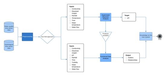
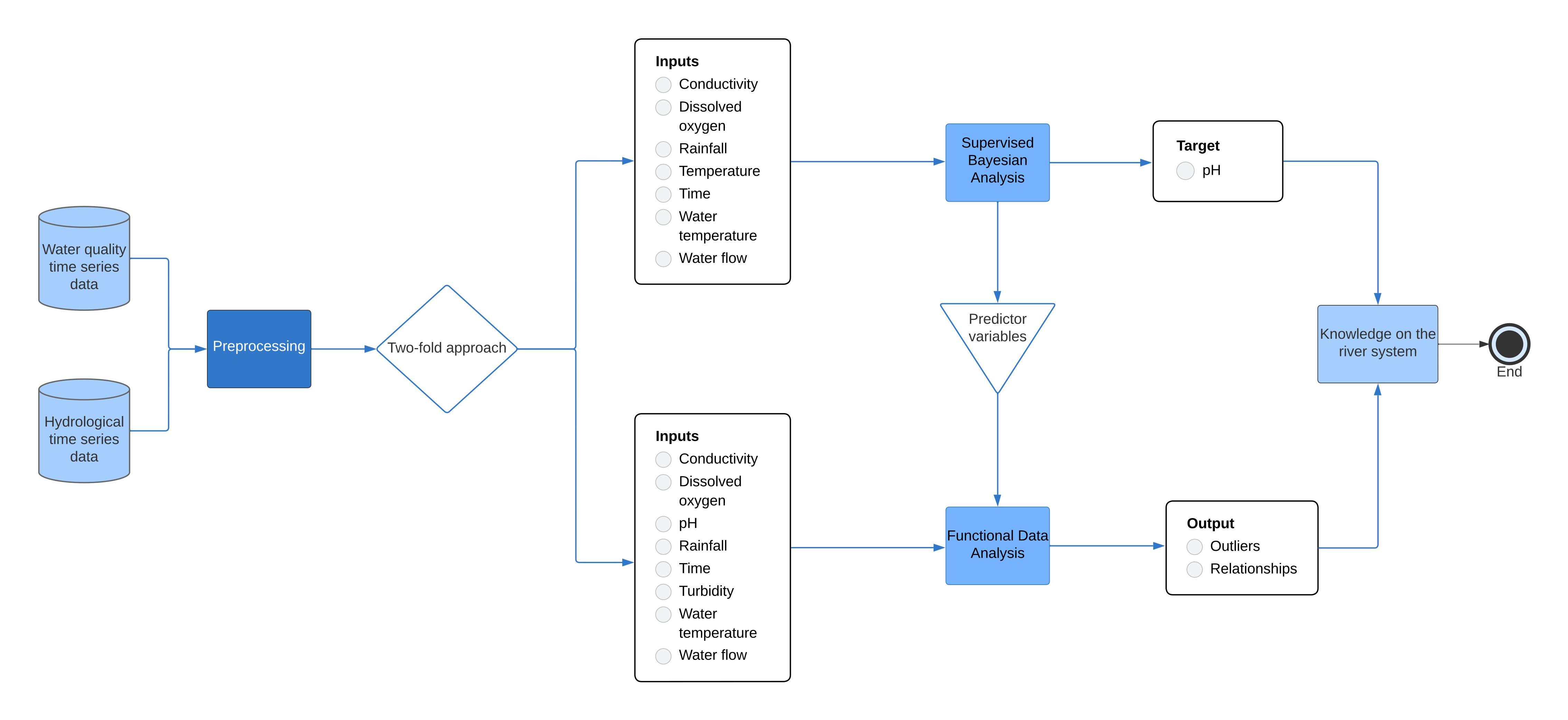
The objective of this research is to evaluate the potential of two advanced mathematical techniques—Bayesian machine learning and functional data analysis—for the analysis and exploitation of knowledge contained in these valuable data series. These models will be implemented to achieve three specific goals: (i) the identification of behavioral patterns of the river systems affected by acid events, (ii) the inference of future behavioral responses, and (iii) the automatic detection of reliable anomalies. Bayesian machine learning models are statistical methods based on uncertainty quantification focused, in this case, on behavioral analysis and inference in complex multivariable systems [17,18,19] such as freshwater systems. On the other hand, functional data analysis [20] is a branch of statistics implemented, in this case, for treating continuous data series and detecting anomalies in different variables [21,22,23,24,25,26,27].
In particular, this research analyzes the case of the Cúa River during the last decade, which runs through the coal mining region of Fabero, located in the NW part of Spain. Mining activity in this area started in the 1910s and ceased definitively in 2018. However, water quality in the Cúa River is still affected by runoff and acid drainage, making it an environmental problem of special interest for the basin management organization. Therefore, the Cúa River is monitored by the two control networks available in this basin. In this work, the results of the Bayesian analysis describe a structure fully dedicated to explaining the behavior of the fluvial system and the characterization of the pH, delving into its statistical association with the rest of the variables in the model. Additionally, the resulting model solves inference problems based on Bayes’ theorem and the calculation of conditional probabilities, which enables predicting future anomalous behaviors of the fluvial system based on the available information from the SAIH and SAICA networks. The main findings of the functional analysis define several time-dependent correlations between the functional outliers of different variables, namely, the inverse relationship between pH, rainfall, and flow.
The novelty of this work is in the implementation and validation of Bayesian networks for: (i) the study of hidden behavioral patterns of the fluvial system dependent on the changes in the pH levels, (ii) the identification of the potential hydrological and physicochemical parameters which regulate these patterns, and (iii) the inference or prediction of future behavior of the fluvial system based on the quantitative variation of its control parameters. Likewise, the FDA algorithms are used for the automatic identification of anomalous events in SAIH and SAICA time series and for their capacity to explain the behavior of the system based on the analysis of anomalous events in their control parameters are validated.
This paper is structured as follows: the first section shows the theoretical framework of the mathematical techniques used and a detailed description of the case study and the data to be processed. Then, the main results of this work are presented in two distinct methodological modules: (i) those resulting from the use of Bayesian models for understanding the behavior of water and inference analysis and (ii) those resulting from the analysis of outliers using functional data analysis. Finally, a discussion of results is carried out to analyze the behavior of the fluvial system based on the results obtained. Lastly, the main conclusions drawn from both study approaches are presented.
2. Materials and Methods
2.1. Fluvial System Description and Data Acquisition
The data analyzed were recorded by a measuring station, which belongs to the SAIH and SAICA networks [13,14], and is located in the Miño-Sil River Basin. Both monitoring systems operate autonomously, collecting data on different variables relative to the control of the fluvial systems in Spain. In particular, the SAIH station measures water flow (m3/s), rainfall (mm), and temperature (), which can affect the biological properties of the aquatic system, as well as the behavior of other substances dissolved in the water.
While the SAICA station records various physicochemical parameters of water quality, including: (i) conductivity (μS/cm), which measures the capacity of an aqueous solution to carry an electric current based on the presence of ions and their concentrations [28], (ii) dissolved oxygen (mg/L), which is essential for the breathing of aquatic organisms and enters the water through diffusion from the atmosphere and as a byproduct of photosynthesis [28], (iii) pH of the water to determine its acidity, using a logarithmic scale ranging from 0 to 14, with values below 7 indicating acidity, and values above 7 indicating basicity [28], and (iv) the amount of suspended particles in the water, known as turbidity (NTU), measured in Nephelometric Turbidity Units to determine the level of cloudiness or muddiness of the water [29].
More specifically, the station was positioned in the Fabero area, in the Alto Bierzo region within the Province of Leon, Spain. Its climate is temperate with a yearly mean temperature of 11.5 , ranging from a mean maximum of 25 in July and a mean minimum in January of 0 . Lastly, the pluviometry in this area is moderate, with a total of 850 mm/year. December and January are the rainiest months, while September and August register the lowest pluviometry values.
The economy of the Fabero region has been heavily influenced by the coal mining industry. The business started in 1917 because of the presence of anthracite coal and did not cease operations until November 2018. The Cúa River and its tributaries are the main hydrological resources of the area, and they are considered of special environmental interest by the water basin organization. The water quality in the area is adversely affected by acid mine drainage resulting from coal mining activities. The dumps containing pyrite undergo natural physical, chemical, and biological alterations, including spontaneous combustion and acid drainage production, releasing heavy metals into the environment and negatively impacting the landscape [30]. Acid drainage resulting from precipitation events reacts with rainwater before flowing to the nearest water body and traveling to the Cúa River, causing a gradual decline in pH and deterioration in water quality, particularly when the pH of most aquatic systems falls below 6, and especially below 5 [1].
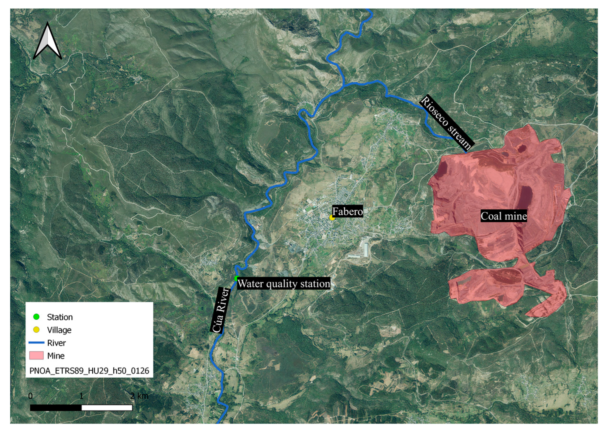
Figure 1 shows a map of the Fabero area, including the location of the largest and last coal mine in the region, the position of the water control station, and the Cúa and Rioseco rivers.
The water quality station, which recorded the data for this research, is located downstream of the main drainage of the coal mine. The data analyzed spans from 1 January 2011 to 31 August 2022, giving a total of 11 years and 8 months recorded with daily frequency. This results in a total of 4342 data points.
2.2. Mathematical Background
The different mathematical methods adopted in this research are introduced in this section. Statistical process control is used as a first approach to identify anomalous events in the data and understand the general behavior of each variable studied; functional data analysis is implemented to achieve reliable detection of outliers and the discovery of relations between them. Lastly, Bayesian machine learning aims to find correlations between different variables and draw inference cases to help model and understand the trends and changes that control the Cúa River's fluvial system.
2.2.1. Statistical Process Control
Statistical process control is defined as the application of a set of statistical methods aiming to monitor and control the quality of a production process. Studying the variation of the data with these methods allows the detection of anomalies within the process. Control charts are the main tool in statistical process control, and they are used to represent and analyze a given process. They were initially created by Walter A. Shewhart [31] in the 1930s.
Significant variations may be easily identified by control charts. However, since they only analyze the most recent samples of groups, control charts fail to detect smaller changes or trends over a considerable time range. In order to address this problem, several new sets of rules were defined [32,33]. In this research, the enhanced version by Lloyd. S. Nelson [34] of the WECO rules [35] was implemented to increase the quality and precision of the results.
2.2.2. Bayesian Networks
Bayesian networks are directed acyclic graphical models (DAGs) that, for a given problem domain, represent a set of variables, called nodes, and their conditional dependencies, called arcs [36]. Their inherently graphical architecture leads to robust models ideal for easily exploring and interpreting complex problems. For the purposes of this study, the BayesiaLab v.10.2 AI software [37] was used to design a supervised Bayesian network based on the collected data in order to optimize the depiction and prediction of water acidification behavior.
To measure the variable impact on the target variable , the relative mutual information (RMI) was calculated to quantify the percentage of knowledge obtained about by observing , thus being able to point out the predictors that give rise to a higher information gain [38]:
where represents the mutual information in absolute terms, and the entropy is an advanced quantification of uncertainty introduced in information theory as the amount of noise or disorder contained in a random variable. Entropy is maximal when all possible states of a distribution are equally likely. On the other hand, if there is no uncertainty, the network has zero entropy [39]. Finally, represents the states of node , and denotes the probability function.
To complete the characterization of the target node, the contributions of each variable to the predicted mean value of the target node were calculated. This metric was derived from counterfactuals based on the analysis of a specific neutral state representing the neutral condition of the system.
Finally, the Contingency Table Fit (CTF) metric was used to measure the quality of the representation of the Joint Probability Distribution (JPD) via the target variable. A common alert threshold below which the target value should be relearned is 70%. From a mathematical viewpoint, CTF may be expressed as [40]:
where represents the entropy value of the constructed Bayesian network, and and are the entropy values of the fully connected and disconnected network, respectively.
2.2.3. Functional Data Analysis
The analysis of functional data is applied to observations of a continuous random process that is observed at discrete points [41]. In the case of an initial sample composed of different data points, the data must be transformed to generate a functional sample. This process consists of defining the best-fitting functions or curves to the initial data points that discretely represent the experimental process. This transformation is known as smoothing.
Considering a set of samples in a set of points , where represents every time instant, all samples can be considered discrete observations of the function , with being a functional space. The function is estimated by taking into account that is a functional space consisting in a set of basis functions , with , where is the required number of basis functions to define the functional space . Several types of basis exist in statistics, but given the fact that the data used in this research has periodic nature, the Fourier basis becomes the most suitable [42,43]. Once the different parameters have been defined, the smoothing problem may be expressed as [26]:
In Equation (3), is the result of evaluating at the point , is the zero-mean random noise, and is an operator which penalizes the complexity of the solution. The purpose of this penalty is to ensure a good fit to the data in the sense that is small, but also some aspect of the data captured by is kept under control. Lastly, the parameter adjusts the intensity of the regularization. After the discrete data is converted to its functional counterpart, outliers, defined as portions of the data that present different parts and/or values, can be detected based on the concept of functional depth. This statistical measure was first introduced for multivariate analysis to quantify the centrality of a given point compared to a set of observations. Consequently, the points represented in a Euclidean space that is close to the center of the distribution will have a greater depth value compared to those located in the periphery [44]. This definition has been extended to the functional domain, where the depth measure analyzes the centrality of a curve compared to a set of curves . Therefore, the concept of depth makes it possible to work with observations, defined in a given time interval, in the form of curves, instead of having to summarize the information contained in these curves into a single value, such as the mean [25]. In this case, the Modified Band Depth (MBD) [45] has been selected as it has demonstrated a better performance in the analysis of environmental data with this approach [46]. Functional directional outlyingness is considered to increase the accuracy in the detection of outliers. This method separates functional outlyingness into two main components: shape outlyingness and magnitude outlyingness, allowing the study of the centrality of the curves and their variability. A magnitude outlier is defined as an observation that is shifted from the mass of the data, while a shape outlier is an observation that differs in shape from the rest of the functions in the set (even if it lies completely inside the bulk of the data) [47]. In this work, the detection of anomalies is performed on the magnitude and shape value pairs according to the outlier detection algorithm introduced by Dai and Genton [48].
3. Results
3.1. Variability of the Data and Outlier Detection with SPC
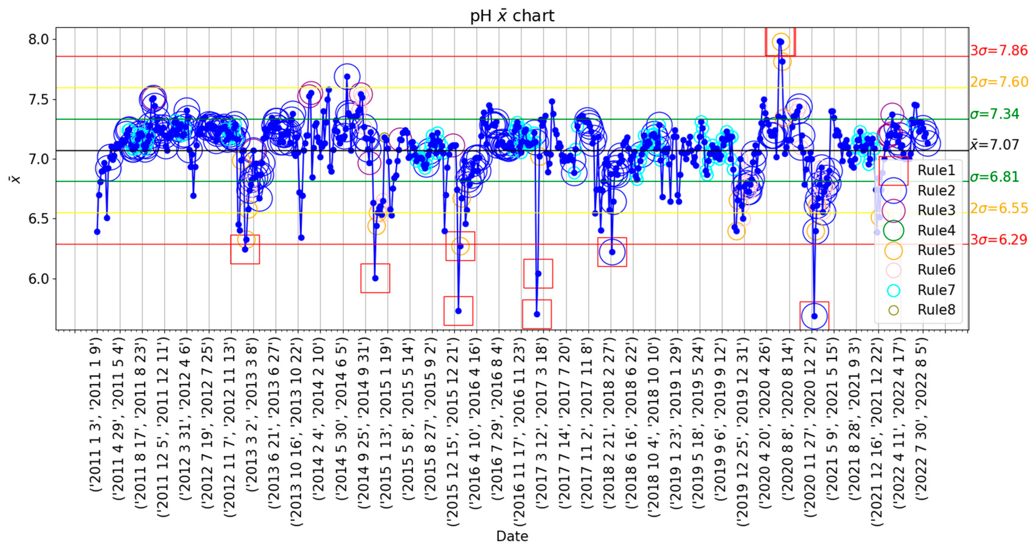
The complete dataset of all variables was initially analyzed with the control chart, which displays the mean of all values in weekly subgroups. Each dot in the plot corresponds to a specific week of the database. Among all variables available, the pH is regarded as the main indicator of the acid mine drainage problem in the Cúa River, while the flow acts as a central measure of the environmental dynamics in the fluvial system. The result of the 8 Nelson rules on the pH control chart is shown in Figure 2. This information helps visualize the data and its variability, besides serving as a first approach to the anomaly detection issue. Nevertheless, the overfitting of the Nelson rules decreases the validity of the results for this purpose.
The pH data, as displayed in the control chart of Figure 3, does not present a clear behavioral cycle, and most values are within 1 standard deviation from the mean. Furthermore, Nelson rule number 1 detects a total of 8 weeks with a pH mean value below 3 standard deviations from the mean and 2 weeks with a mean value over 7.86, which is 3 standard deviations above the mean. Nevertheless, the rest of the rules detect an unrealistic number of alarms, as it represents more than 50% of the pH data.
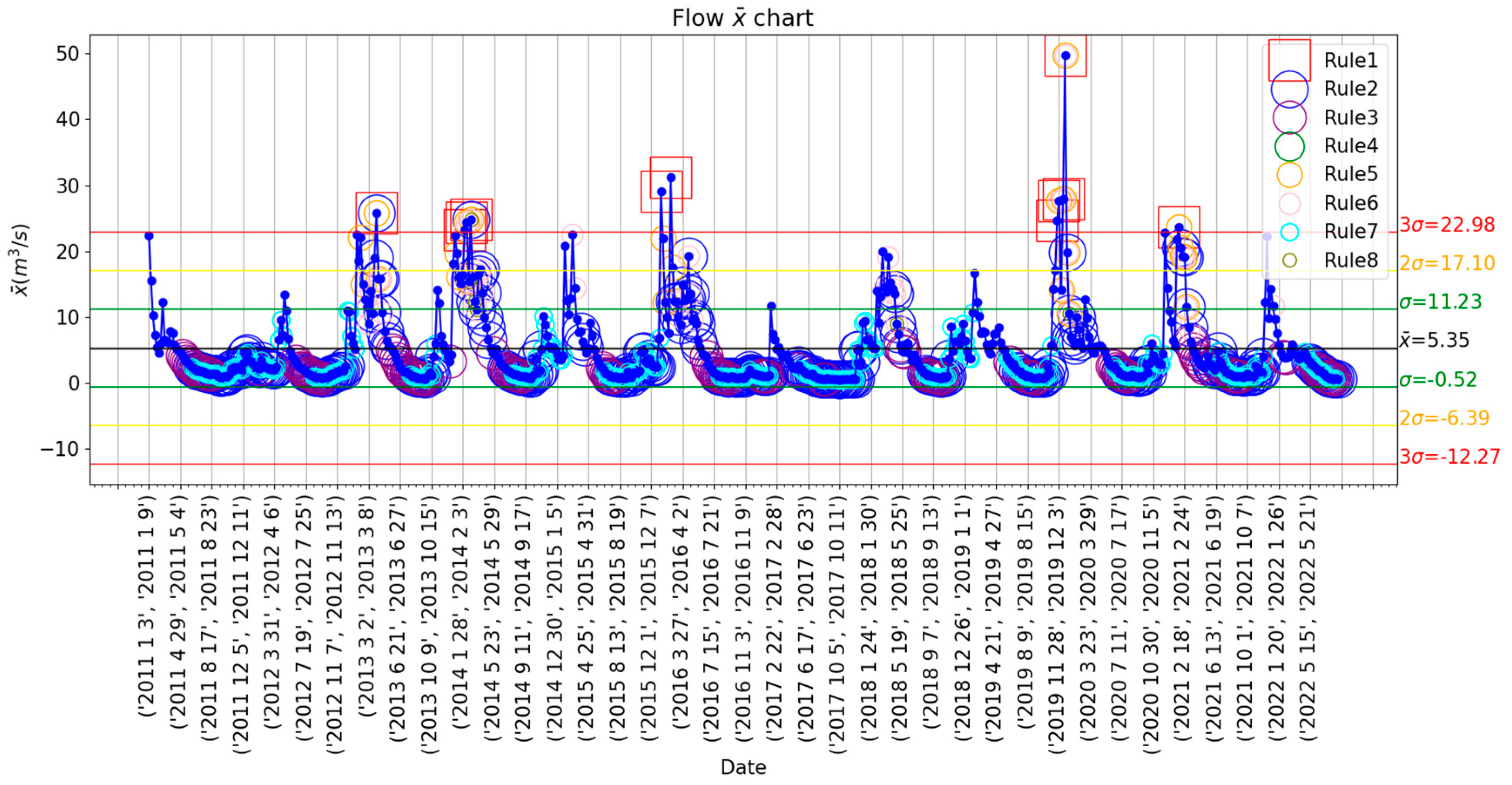
Another example of this analysis is presented in Figure 3. In this case, the variable water flow is analyzed with the control chart. Contrary to the pH data, the water flow displays a clear pattern, marked by a fast increase from December until reaching peak values in the winter months of the Northern Hemisphere and a steep decline in spring to the low and steady water flow levels of the remainder of the year. Additionally, Nelson rule number 1 performs a correct detection of the most outstanding anomalies in accordance with the functional results, but rules number 2 and 3 define as outliers a disproportionate number of weeks, mostly, all those values below the mean which correspond to normal flow in the months of summer, fall, and the end of spring.
Consequently, the results of the statistical process control do not present a degree of reliability high enough for accurate anomaly detection in these data. However, they shed light on its variability, the seasonal patterns of the Cúa River, and the different standard deviation intervals defined, which will be used to classify individual values in different categories in the Bayesian analysis.
3.2. Variables Influence Analysis in pH Distribution
In this section, a supervised Bayesian network representing the general problem under study was constructed by analyzing the statistical association stemming from the pH status and each variable in the model. For that, considering the entire database, the standard deviation intervals defined from the control charts of each variable in the database were used as discretization threshold values for the Bayesian analysis (Table 1).
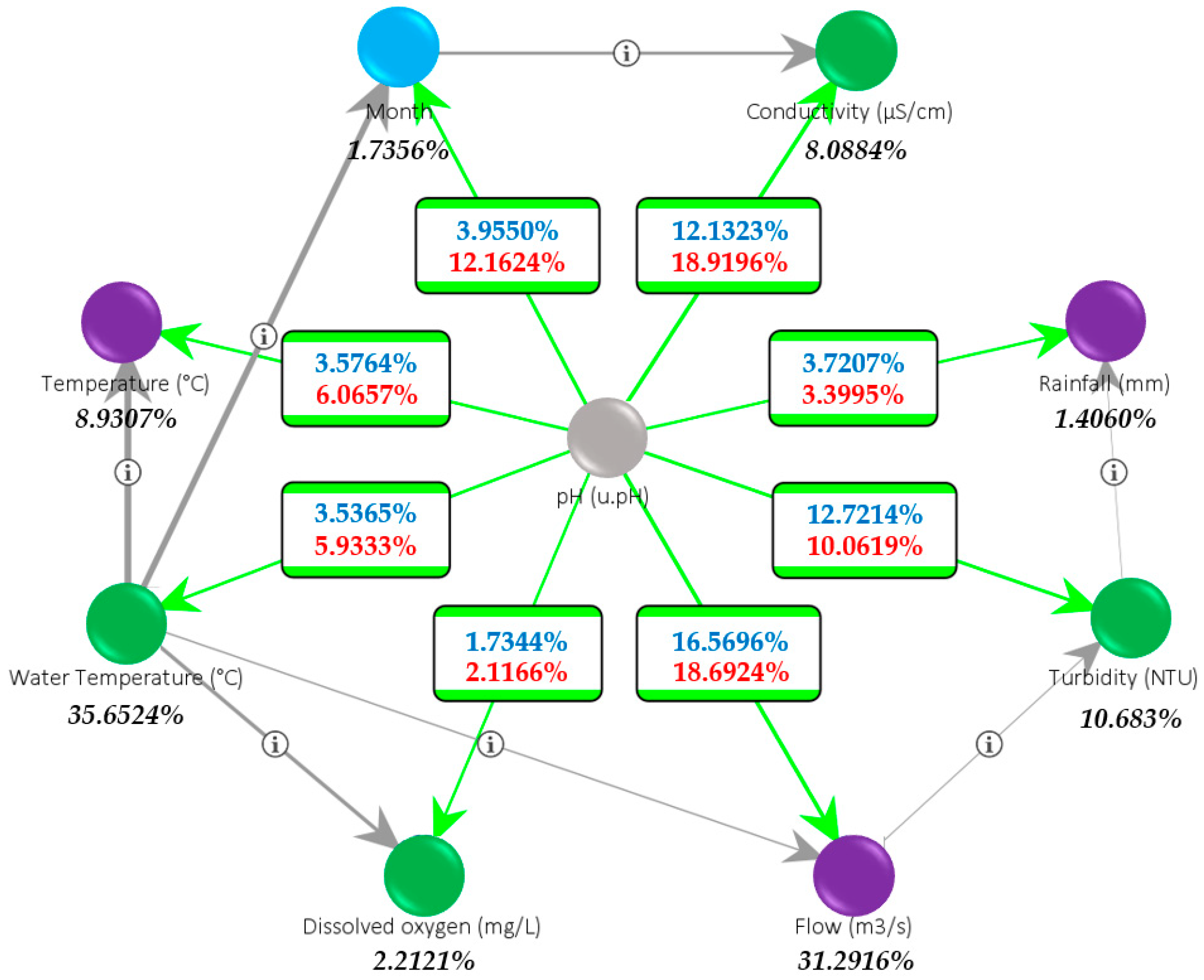
From the resulting Bayesian network, a relationship analysis was carried out, between the target node (pH) and its child nodes, with the goal of identifying the most representative parent–child connections. These relationships are shown in Figure 4, where water temperature (35.65%) and flow (31.29%) stand out for their high impact, followed by turbidity (10.68%), air temperature (8.93%), and conductivity (8.09%) variables. To clarify the interpretation, the RMI was also computed exclusively between the arcs of the variables and the target node. The blue number shows the RMI concerning the secondary node, while the red number refers to the main node. Thus, knowing the pH state reduces the uncertainty of the conductivity characteristics by 18.9196%. In the opposite direction, river flow is the factor that provides the most significant reduction in the uncertainty of the pH state (16.5696%). Similar results are found for turbidity and conductivity, with 12.7214% and 12.1323%, respectively. From the point of view of the predictive importance of the variables, dissolved oxygen is the factor that provides the lowest amount of information in the case analyzed.
To go deeper into the problem of acid mine drainage in the Cúa River, Table 2 presents the calculation of the amount of information brought by each variable to the knowledge of the different ranges of pH values. Previous high-impact studies have shown that freshwater quality begins to gradually deteriorate as we move away from the normal value (). This deterioration in water acceptability is most noticeable when pH values fall below 6 and, in particular, below 5 [1]. Likewise, for maximum productivity, Simate and Ndluvo emphasize that the pH value range be maintained between 6.5 and 8.5 [1].
That said, this local analysis between each of the 4 states of the target variable and its predictors allowed us to identify that flow in pH ranges below 5.5 [49] is the factor with the highest correlation. Given the importance of freshwater quality when the pH value drops below 6.5, the percentage values of mutual information obtained for conductivity, flow, turbidity, and month variables in the pH range between 5.5 and 6.5 should be highlighted. However, if the pH level is higher than 7.1, the most important predictor variables would be conductivity (20.361%) and flow rate (19.603%), respectively.
In terms of model validation, CTF is a very useful metric to measure the quality of the JPD representation. A CTF higher than 70% implies an adequate quality of the induced factors, and specifically the value obtained for the supervised Bayesian network created is 74.581%.
3.3. Functional Analysis Approach
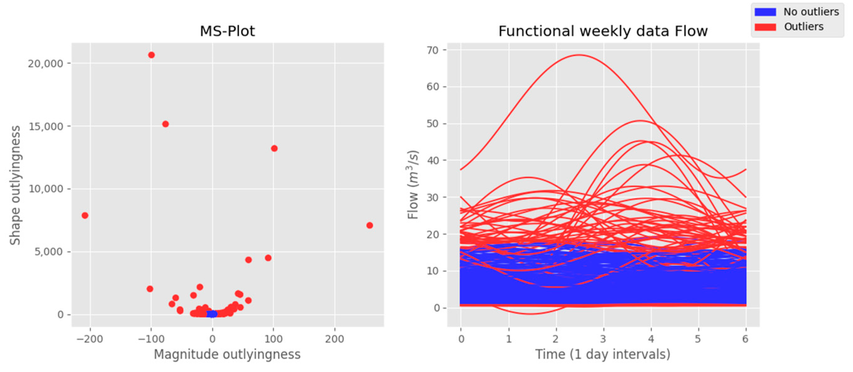
This section presents the results of the functional analysis of each variable for outlier detection purposes. Most notably, several relationships are drawn between two or three given variables of the database related to the date of their respective outliers. In accordance with the results of the mutual information analysis between each variable and the pH, the functional results begin with the analysis of the water flow variable, whose graphical results are displayed in Figure 5. The left side of this figure contains a Cartesian representation of the magnitude–shape pair of values of each function. As can be seen, those functions with an anomalous magnitude and/or shape outlyingness value (red points) lay outside the main cluster of points, which contains the pair of values magnitude-shape of the nonoutlying functions (blue points). The right side shows the functional plot of the weekly rainfall values. Those functions that are considered anomalous are colored in red, while those considered standard are represented in blue. Water flow has a mean value of 5.35 m3/s, with a maximum of 67.37 m3/s on 20 December 2019, and a minimum of 0.46 on 9 October 2017, with most outliers taking place between December and March of every year.
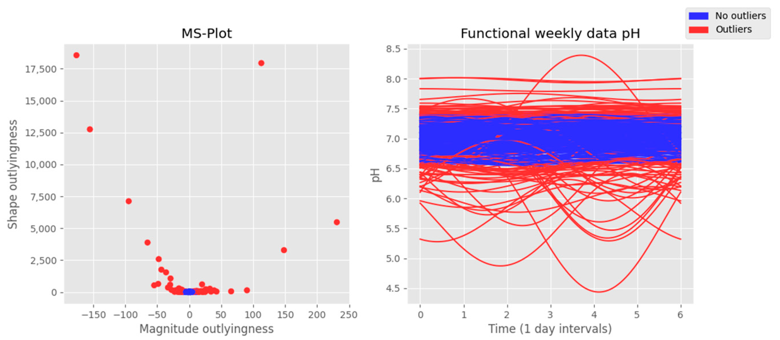
Furthermore, Figure 6 shows the results of the functional analysis on the pH data in the same fashion as the previous image. This variable has an average value of 7.07 with a minimum of 4.3 on 5 February 2017, and a maximum of 8.0 on several days in June and July 2020, with most acid anomalies happening also between December and March.
This analysis was performed on the data of each variable, and the results are summarized in Table 3. This table contains basic statistics of all variables analyzed and the number of weeks identified as functional outliers.
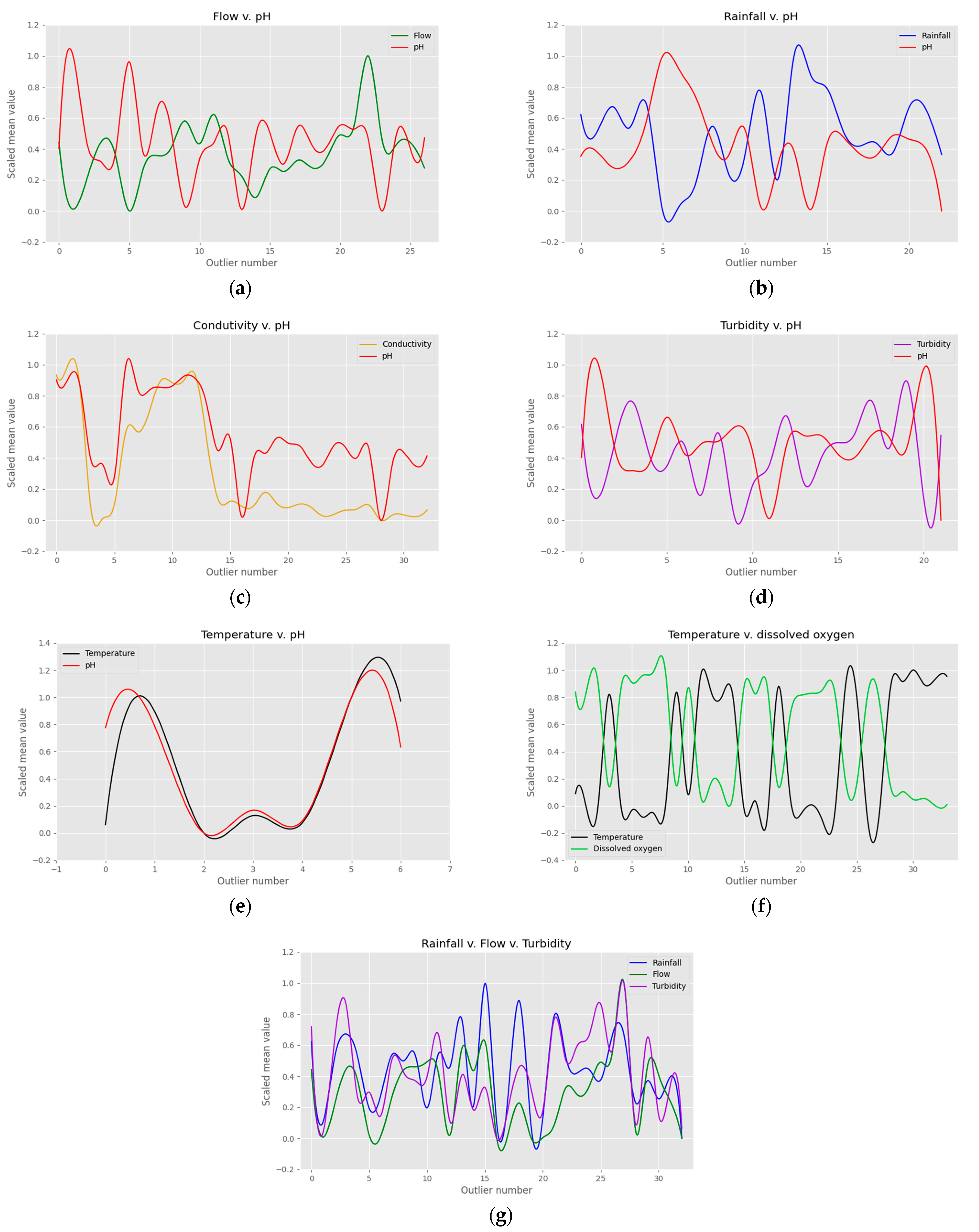
After the functional outliers are detected, it can be inferred that there could be some degree of correlation between the variables, as the number of outliers is around the same value in all cases. The existence of anomalous events on the same dates and in several variables defines a multivariate anomaly, and its detection validates the functional analysis for the identification of such events in the data provided by the SAIH and SAICA networks. These results are complemented with a time dependency analysis of the detected outliers and the correlations between the different variables. The rest of this section presents the relationships found between two or more variables based on the anomaly detection results of the functional analysis. The main outlier correlations found are presented graphically in Figure 7.
Flow and pH contain 26 coincidental outlying weeks, giving a match percentage of 32% between those 2 variables. They present an inverse relationship since when the flow increases, the pH levels drop. Weeks from numbers 17 to 20 seem to break away from the defined trend. However, these weeks, which belong to November and December 2019, present mean flow levels between 14.31 m3/s and 24.71 m3/s. Consequently, their values are considerably above the 3rd quartile of the flow data, which is 6.53 m3/s, evidencing their outlying behavior. This information points towards the fact that the pH level can decrease, but when it reaches a certain point, the water flow loses its influence. In other words, there are certain scenarios when an increase in the flow level will not necessarily imply a further drop in the pH.
Rainfall and pH have a total of 23 outlying weeks in common, which translates into a 28% match. It can be observed that their relationship is inverse, meaning that when it rains, the pH levels drop. Nevertheless, there is an exception to this rule: outlying week number 22 (10 December 2020 16 December 2020), when the rainfall values decrease in synchronization with the pH levels. This behavior is explained by analyzing the precipitation levels in the previous week, which are around a high value of 7.1 mm each day. Additionally, in week number 22, there is a peak of 17 mm and 26 mm on Monday and Tuesday, but Wednesday, Thursday, and Friday are close to 0 mm, lowering the mean value of that week. Thus, it can be inferred that when a precipitation event takes place, the pH levels do not drop immediately, and when the rain ceases, the pH level does not go back up to its standard numbers after at least 3 to 7 days.
Turbidity and pH present an inverse relationship, which matches with the behavior of the fluvial system, meaning that a higher level of dissolved particles implies acid waters with a lower pH value. The correlation between these 2 variables translates into a matching percentage of 27% with 21 outlying weeks shared between turbidity and pH. Conductivity and pH have a clean direct relationship: when the conductivity decreases, so does the pH and vice versa. These 2 variables have a matching percentage of 40% with a total of 32 coincidental anomalous weeks. Temperature and pH have 6 outlying weeks in common, resulting in a matching percentage of 9%. Nevertheless, their proper direct relationship can be observed in Figure 7e.
Temperature and dissolved oxygen include a higher number of common outliers for a total of 33, resulting in a match percentage of 41% and a well-defined inverse relationship since when the temperature rises, especially in the summer months, the dissolved oxygen declines. Lastly, three variables were found to have a direct relationship: rainfall, flow, and turbidity. They present a matching percentage of 40% due to their 32 coincidental outliers. This relationship can be seen in Figure 7g.
Paying close attention to the pH variable, which is paramount in this analysis, the total number of outliers explained by the relationship between the pH and any of the other 6 variables in the database is 55, equivalent to 65% of the pH anomalies. This implies that there is a 35%, or 29 outliers, of the 84 total pH anomalies unexplained by their correlations with the other variables. Out of these 29 outliers, 24 are weeks with a mean value above the average. Therefore, these anomalies, of which 61% take place in the driest months of the year between May and October, could be due to a natural process whose information is not contained in the current variables available or due to uncontrolled dumps of polluting elements in the Cúa River. Regarding the 5 outliers remaining unexplained, these present a mean value lower than the mean pH of 7.07, but after careful analysis of the rainfall in the weeks prior and after those anomalies, it can be concluded that there is some lag between the rainfall anomaly and the associated acid pH outlier. In these circumstances, every time an important precipitation begins, the acid pH anomaly does not take place until approximately 1.5 days on average have passed. Similarly, when the rainfall stops, it still takes typically 4.5 days for the pH levels to rise.
4. Discussion
The hydrological and environmental data of the Cúa River was analyzed with three different statistical methods. The results of the control charts, in particular, the chart provides valuable information on the variability of data, the seasonality of the different natural processes taking place in the river, and the different standard deviation intervals defined by the control limits. On the other hand, the detection of anomalies through this method does not offer consistent results. Control charts consider the temporal correlation between data, but even when the use of subgroups is helpful for graphical representation, it also accounts for an important loss of information. Additionally, the seasonality of the environmental data damages the performance of these methods as the anomaly detection rules become erratic. It is this set of conditions that leads to the detection of an unrealistic number of outliers, marked by the definition of frequent values as anomalies.
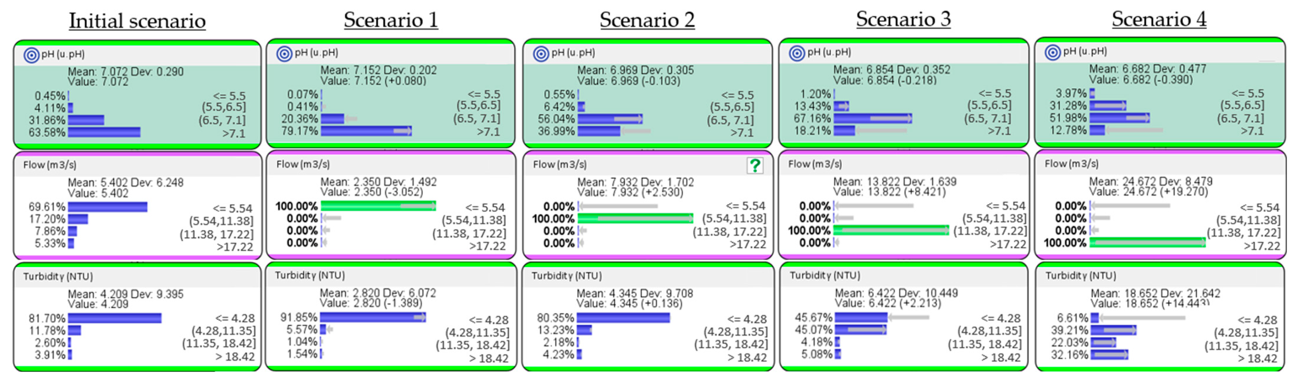
Concerning Bayesian analysis, the use of artificial intelligence algorithms in combination with other mathematical approaches is expected to have a positive impact on public water protection policies in the coming years. These models have a high capacity and flexibility for the analysis of complex problems and can handle the heterogeneity of hydrological circumstances. As an example of the potential of this combined approach, Figure 8 shows the Bayesian results of an inference analysis on the target node pH, the physical variable flow, and the chemical node turbidity. Overall, the results reveal the direct relationship of pH with flow rate, with a nearly 9-fold increase in the probabilities of pH < 5.5 occurring if the water flow rate was high (x + 2σ). Furthermore, as it is consistent, a potential change in water turbidity regimes was detected when the flow rate increases above 17.22 m3/s.
The functional analysis approach studies the whole process and extracts continuous information from the dataset, which translates into a much smaller loss of information and a reliable study of the different trends in the data. Additionally, the smoothing process, which transforms the discrete data into functions, achieves a precise approximation of the original data points enhancing the elimination of erroneous values, such as failures in the data-gathering sensors.
The results of the functional approach automatically identify a series of outliers in each variable. A time-dependency analysis was implemented to assess the reliability of the detected outliers. This process reveals that, on average, several variables present 31% outliers on the same dates. Additionally, studying the values of those anomalies in each correlated variable reveals hidden correlations between them. Most interesting is the case of water flow, rainfall, and turbidity, which are inversely correlated with the pH and present. On the other hand, conductivity shows a direct relationship with the pH, which seems to be a particular behavior of this fluvial system. Consequently, these results validate the functional approach for the automatic detection of outliers and the modeling of a fluvial system based on the time series data collected by the SAIH and SAICA water control networks.
5. Conclusions
The occurrence of acid mine drainage events in the Cúa River (NW part of Spain) was analyzed through statistical process control, Bayesian machine learning, and functional data analysis. The data studied were recorded by a water control station in the Cúa River with daily records of conductivity, dissolved oxygen, pH, rainfall, temperature, turbidity, and water flow between January 2011 and August 2022.
Statistical process control acts as a first approach to the problem. This method takes into account the time correlations within the data due to the use of rational subgroups, but this implies the loss of information. Adding the lack of normality, and high variability of the data, the results end up being plagued with false alarms. Nevertheless, the chart provides valuable information regarding the variability of the parameters that control water quality in the Cúa River, as well as the different standard deviation intervals for each variable, which are leveraged by the Bayesian analysis.
The Bayesian model can achieve a higher degree of understanding of the behavior of the fluvial system. A valuable measure for evaluating the effectiveness of the JPD representation among the monitored variables, known as CTF, was calculated. The resulting CTF of 74.581% means that the model provides an accurate representation of the behavior of the aquatic system. In order to know in which potential ranges of values the pH will be found, the calculation of the RMBI between pH states and their predictor variables revealed the most important variables to watch out for. The results showed that for pH ranges below the lower limit set in the RD 817/2015, the potential predictors were flow, month, and turbidity of the water.
Lastly, the functional approach is not dependent on the statistical distribution of the data and studies it as a complete time unit, which leads to better trend analysis, a reduction in the information lost in the process, and more refined outlier detection. The validation of the functional results was carried out through a multivariate temporal analysis of the detected anomalies. Several correlations were found by taking a closer look at the time dependency between the outliers of the different variables. In particular, the variable rainfall presents a direct relationship with the increase of the water flow and the turbidity of the fluvial system, as well as the decrease in the pH and conductivity levels. Additionally, the temporal analysis showed that in some cases, the pH levels do not fall right at the beginning of a precipitation event; rather, they decrease typically 1.5 later and remain low for 4.5 days on average despite the precipitation event having been completed.
It is worth noting that the methods used adapt effectively to the data collected continuously by the hydrological and water quality monitoring networks installed in the study area. This makes it possible to analyze and comprehend the specific behavior of a river over an interval of time, as well as draw inference scenarios and automatically detect reliable multivariate outliers between the different variables studied.
The reliability of the methods implemented is dependent on the availability of time series data without significant portions of missing values. As with most statistical methods, the absence of continuity can translate into a negative impact on the accuracy of the models; therefore, the obtention of faithful results is heavily dependent on the adequate maintenance of the monitoring networks. The national authorities in charge of the protection of water quality in this river basin are planning the development of specific actions with the intent to treat water in the event of acidic conditions. Thus, this study may be an interesting and powerful tool to identify anomalous events and to establish and determine the requirements of future treatments.
Author Contributions
Conceptualization, M.A. and S.G.; methodology, X.R. and M.P.; software, X.R. and M.P.; validation, X.R., M.P., M.A. and E.B.; formal analysis, X.R. and M.P.; investigation, X.R. and M.P.; resources, X.R. and M.P.; data curation, X.R. and M.P.; writing—original draft preparation, X.R. and M.P.; writing—review and editing, X.R. and M.P.; visualization, X.R.; supervision, M.A., S.G. and E.B.; project administration, M.A.; funding acquisition, M.A. All authors have read and agreed to the published version of the manuscript.
Funding
This research was funded by the Spanish Ministry of Science and Innovation (MCIN/AEI/10.13039/501100011033), grant number PID2020-116013RB-I00.
Data Availability Statement
The data analyzed in this study is publicly available here https://github.com/xrigueira/data/tree/main/water/Cua (accessed on 20 March 2023).
Conflicts of Interest
The authors declare no conflict of interest. The funders had no role in the design of this study; in the collection, analyses, or interpretation of data; in the writing of the manuscript; or in the decision to publish the results.
References
- Simate, G.S.; Ndlovu, S. Acid Mine Drainage: Challenges and Opportunities. J. Environ. Chem. Eng. 2014, 2, 1785–1803. [Google Scholar] [CrossRef]
- Akcil, A.; Koldas, S. Acid Mine Drainage (AMD): Causes, Treatment and Case Studies. J. Clean. Prod. 2006, 14, 1139–1145. [Google Scholar] [CrossRef]
- Monterroso, C.; Macías, F. Drainage Waters Affected by Pyrite Oxidation in a Coal Mine in Galicia (NW Spain): Composition and Mineral Stability. Sci. Total Environ. 1998, 216, 121–132. [Google Scholar] [CrossRef]
- Tiwary, R.K. Environmental Impact of Coal Mining on Water Regime and Its Management. Water. Air. Soil Pollut. 2001, 132, 185–199. [Google Scholar] [CrossRef]
- Campaner, V.P.; Luiz-Silva, W.; Machado, W. Geochemistry of Acid Mine Drainage from a Coal Mining Area and Processes Controlling Metal Attenuation in Stream Waters, Southern Brazil. An. Acad. Bras. Cienc. 2014, 86, 539–554. [Google Scholar] [CrossRef] [PubMed]
- Alhamed, M.; Wohnlich, S. Environmental Impact of the Abandoned Coal Mines on the Surface Water and the Groundwater Quality in the South of Bochum, Germany. Environ. Earth Sci. 2014, 72, 3251–3267. [Google Scholar] [CrossRef]
- Kicińska, A.; Pomykała, R.; Izquierdo-Diaz, M. Changes in Soil PH and Mobility of Heavy Metals in Contaminated Soils. Eur. J. Soil Sci. 2022, 73, e13203. [Google Scholar] [CrossRef]
- Nordstrom, D.K. Hydrogeochemical Processes Governing the Origin, Transport and Fate of Major and Trace Elements from Mine Wastes and Mineralized Rock to Surface Waters. Appl. Geochem. 2011, 26, 1777–1791. [Google Scholar] [CrossRef]
- Kim, J.J.; Kim, S.J. Seasonal Factors Controlling Mineral Precipitation in the Acid Mine Drainage at Donghae Coal Mine, Korea. Sci. Total Environ. 2004, 325, 181–191. [Google Scholar] [CrossRef]
- Masindi, V. Recovery of Drinking Water and Valuable Minerals from Acid Mine Drainage Using an Integration of Magnesite, Lime, Soda Ash, CO2 and Reverse Osmosis Treatment Processes. J. Environ. Chem. Eng. 2017, 5, 3136–3142. [Google Scholar] [CrossRef]
- Wright, I.A.; Paciuszkiewicz, K.; Belmer, N. Increased Water Pollution After Closure of Australia′s Longest Operating Underground Coal Mine: A 13-Month Study of Mine Drainage, Water Chemistry and River Ecology. Water Air. Soil Pollut. 2018, 229, 55. [Google Scholar] [CrossRef]
- Hobbs, P.; Oelofse, S.H.H.; Rascher, J. Management of Environmental Impacts from Coal Mining in the Upper Olifants River Catchment as a Function of Age and Scale. Int. J. Water Resour. Dev. 2008, 24, 417–431. [Google Scholar] [CrossRef]
- MITECO SAIH Network. Available online: https://www.miteco.gob.es/es/agua/temas/evaluacion-de-los-recursos-hidricos/SAIH/ (accessed on 8 November 2022).
- MITECO SAICA Network. Available online: https://www.miteco.gob.es/es/agua/temas/estado-y-calidad-de-las-aguas/aguas-superficiales/programas-seguimiento/saica.aspx (accessed on 12 November 2022).
- Yaroshenko, I.; Kirsanov, D.; Marjanovic, M.; Lieberzeit, P.A.; Korostynska, O.; Mason, A.; Frau, I.; Legin, A. Real-Time Water Quality Monitoring with Chemical Sensors. Sensors 2020, 20, 3432. [Google Scholar] [CrossRef] [PubMed]
- Sambito, M.; Freni, G. Strategies for Improving Optimal Positioning of Quality Sensors in Urban Drainage Systems for Non-Conservative Contaminants. Water 2021, 13, 934. [Google Scholar] [CrossRef]
- Ajami, N.K.; Hornberger, G.M.; Sunding, D.L. Sustainable Water Resource Management under Hydrological Uncertainty. Water Resour. Res. 2008, 44, W11406. [Google Scholar] [CrossRef] [Green Version]
- Ovaskainen, O.; Tikhonov, G.; Norberg, A.; Guillaume Blanchet, F.; Duan, L.; Dunson, D.; Roslin, T.; Abrego, N. How to Make More out of Community Data? A Conceptual Framework and Its Implementation as Models and Software. Ecol. Lett. 2017, 20, 561–576. [Google Scholar] [CrossRef] [Green Version]
- Gokdemir, C.; Li, Y.; Rubin, Y.; Li, X. Stochastic Modeling of Groundwater Drawdown Response Induced by Tunnel Drainage. Eng. Geol. 2022, 297, 106529. [Google Scholar] [CrossRef]
- Ramsay, J.O.; Silverman, B.W. Functional Data Analysis, 2nd ed.; Springer New York LLC: New York, NY, USA, 2005; ISBN 978-0-387-40080-8. [Google Scholar]
- Febrero, M.; Galeano, P.; Gonz, W. Outlier Detection in Functional Data by Depth Measures, with Application to Identify Abnormal NOx Levels. Environmetrics 2008, 19, 331–345. [Google Scholar] [CrossRef]
- Sancho, J.; Martínez, J.; Pastor, J.J.; Taboada, J.; Piñeiro, J.I.; García-Nieto, P.J. New Methodology to Determine Air Quality in Urban Areas Based on Runs Rules for Functional Data. Atmos. Environ. 2014, 83, 185–192. [Google Scholar] [CrossRef]
- Sancho, J.; Iglesias, C.; Piñeiro, J.; Martínez, J.; Pastor, J.J.; Araújo, M.; Taboada, J. Study of Water Quality in a Spanish River Based on Statistical Process Control and Functional Data Analysis. Math. Geosci. 2016, 48, 163–186. [Google Scholar] [CrossRef]
- Sancho, J.; Pastor, J.J.; Martínez, J.; García, M.A. Evaluation of Harmonic Variability in Electrical Power Systems through Statistical Control of Quality and Functional Data Analysis. Procedia Eng. 2013, 63, 295–302. [Google Scholar] [CrossRef] [Green Version]
- Martínez Torres, J.; Pastor Pérez, J.; Sancho Val, J.; McNabola, A.; Martínez Comesaña, M.; Gallagher, J. A Functional Data Analysis Approach for the Detection of Air Pollution Episodes and Outliers: A Case Study in Dublin, Ireland. Mathematics 2020, 8, 225. [Google Scholar] [CrossRef] [Green Version]
- Martínez Torres, J.; Garcia Nieto, P.J.; Alejano, L.; Reyes, A.N. Detection of Outliers in Gas Emissions from Urban Areas Using Functional Data Analysis. J. Hazard. Mater. 2011, 186, 144–149. [Google Scholar] [CrossRef]
- Ordóñez, C.; Martínez, J.; de Cos Juez, J.F.; Sánchez Lasheras, F. Comparison of GPS Observations Made in a Forestry Setting Using Functional Data Analysis. Int. J. Comput. Math. 2012, 89, 402–408. [Google Scholar] [CrossRef]
- Gorde, S.P.; Jadhav, M.V. Assessment of Water Quality Parameters: A Review. Int. J. Eng. Res. Appl. 2013, 3, 2029–2035. [Google Scholar]
- Kitchener, B.G.B.; Wainwright, J.; Parsons, A.J. A Review of the Principles of Turbidity Measurement. Prog. Phys. Geogr. 2017, 41, 620–642. [Google Scholar] [CrossRef] [Green Version]
- Ribeiro, J.; Ferreira da Silva, E.; Li, Z.; Ward, C.; Flores, D. Petrographic, Mineralogical and Geochemical Characterization of the Serrinha Coal Waste Pile (Douro Coalfield, Portugal) and the Potential Environmental Impacts on Soil, Sediments and Surface Waters. Int. J. Coal Geol. 2010, 83, 456–466. [Google Scholar] [CrossRef]
- Shewhart, W.A. Economic Control of Quality of Manufactured Product; Van Nostrand Company, Inc.: New York, NY, USA, 1931. [Google Scholar]
- Champ, C.W.; Woodall, W.H. Exact Results for Shewhart Control Charts with Supplementary Runs Rules. Technometrics 1987, 29, 393–399. [Google Scholar] [CrossRef]
- Zhang, S.; Wu, Z. Designs of Control Charts with Supplementary Runs Rules. Comput. Ind. Eng. 2005, 49, 76–97. [Google Scholar] [CrossRef]
- Nelson, L.S. The Shewhart Control Chart—Tests for Special Causes. J. Qual. Technol. 1984, 16, 237–239. [Google Scholar] [CrossRef]
- Electric, W. Statistical Quality Control Handbook; Western Electric Corporation: Indianapolis, Indiana, 1956. [Google Scholar]
- Conrady, S.; Jouffe, L. Bayesian Networks and BayesiaLab—A Practical Introduction for Researchers, 1st ed.; Bayesia USA: Franklin, TN, USA, 2015; ISBN 0996533303. [Google Scholar]
- S.A.S., B. BayesiaLab 2022. Available online: https://www.bayesia.com/articles/#!bayesialab-knowledge-hub/2022-bayesialab-conference (accessed on 20 January 2023).
- Shannon, C.E. A Mathematical Theory of Communication. Bell Syst. Tech. J. 1948, 27, 379–423. [Google Scholar] [CrossRef] [Green Version]
- Radicchi, F.; Krioukov, D.; Hartle, H.; Bianconi, G. Classical Information Theory of Networks. J. Phys. Complex. 2020, 1, 25001. [Google Scholar] [CrossRef]
- S.A.S., B. Contingency Table Fit. Available online: https://www.bayesia.com/articles/#!bayesialab-knowledge-hub/key-concepts-contingency-table-fit (accessed on 22 January 2023).
- Ramsay, J.O.; Silverman, B.W. Functional Data Analysis, 1st ed.; Springer International Publishing: New York, NY, USA, 2002; ISBN 9781461271666. [Google Scholar]
- Di Blasi, J.I.P.; Martínez Torres, J.; García Nieto, P.J.; Alonso Fernández, J.R.; Díaz Muñiz, C.; Taboada, J. Analysis and Detection of Outliers in Water Quality Parameters from Different Automated Monitoring Stations in the Miño River Basin (NW Spain). Ecol. Eng. 2013, 60, 60–66. [Google Scholar] [CrossRef]
- Díaz Muñiz, C.; García Nieto, P.J.; Alonso Fernández, J.R.; Martínez Torres, J.; Taboada, J. Detection of Outliers in Water Quality Monitoring Samples Using Functional Data Analysis in San Esteban Estuary (Northern Spain). Sci. Total Environ. 2012, 439, 54–61. [Google Scholar] [CrossRef] [PubMed]
- Martínez, J.; Saavedra, Á.; García-Nieto, P.J.; Piñeiro, J.I.; Iglesias, C.; Taboada, J.; Sancho, J.; Pastor, J. Air Quality Parameters Outliers Detection Using Functional Data Analysis in the Langreo Urban Area (Northern Spain). Appl. Math. Comput. 2014, 241, 1–10. [Google Scholar] [CrossRef]
- Lopez-Pintado, S.; Romo, J. On the Concept of Depth for Functional Data. J. Am. Stat. Assoc. 2009, 104, 718–734. [Google Scholar] [CrossRef] [Green Version]
- Rigueira, X.; Araújo, M.; Martínez, J.; García-Nieto, P.J.; Ocarranza, I. Functional Data Analysis for the Detection of Outliers and Study of the Effects of the COVID-19 Pandemic on Air Quality: A Case Study in Gijón, Spain. Mathematics 2022, 10, 2374. [Google Scholar] [CrossRef]
- Ojo, O.; Lillo, R.E.; Anta, A.F. Outlier Detection for Functional Data with R Package Fdaoutlier. arXiv 2021. [Google Scholar] [CrossRef]
- Dai, W.; Genton, M.G. Multivariate Functional Data Visualization and Outlier Detection. J. Comput. Graph. Stat. 2018, 27, 923–934. [Google Scholar] [CrossRef] [Green Version]
- Ministerio del Ambiente, Agua y Transición Ecológica. Real Decreto 817/2015, de 11 de septiembre, Por El Que Se Establecen Los Criterios de Seguimiento y Evaluación Del Estado de Las Aguas Superficiales y Las Normas de Calidad Ambiental. Available online: https://www.boe.es/eli/es/rd/2015/09/11/817 (accessed on 22 January 2023).
Figure 1.
The geographical location of Fabero marked with a yellow dot, the coal mine in red, positioned to the east of Fabero, the water control station in green, and the two main rivers in the area: Cúa and Rioseco in blue.
Figure 1.
The geographical location of Fabero marked with a yellow dot, the coal mine in red, positioned to the east of Fabero, the water control station in green, and the two main rivers in the area: Cúa and Rioseco in blue.

Figure 2.
pH data represented in the control chart with weekly rational subgroups and the 8 Nelson rules implemented for outlier detection, trend study, and variability analysis. The mean of all subgroups is represented by a black line, while the green, yellow, and red lines mark the , and limits, respectively.

Figure 3.
Flow data is represented in the control chart with weekly rational subgroups and the Nelson rules implemented for outlier detection, trend study, and variability analysis. The mean of al subgroup is represented by a black line, while the green, yellow, and red lines mark the , and limits, respectively.

Figure 4.
Supervised BN built with Augmented Naïve Bayes algorithm. The graph presents a radial layout with the target node (pH) in the center. The color of the nodes represents the type of variable: chemical, physical, or temporal. The values of the arcs correspond to the RMI (%) analyses, and the values of the nodes are the variable contributions to the target node (%).

Figure 5.
Results of the functional analysis on the water flow data. On the left side, a Cartesian representation of the pair of values magnitude–shape of each function is presented. The right side shows the functional plot of the weekly water flow values. Outliers are marked in red in both plots, and nonoutliers are colored in blue.

Figure 6.
Results of the functional analysis on the pH data. On the left side, a Cartesian representation of the pair of values magnitude–shape of each function is presented. The right side shows the functional plot of the weekly pH values. Outliers are marked in red in both plots, and nonoutliers are colored in blue.

Figure 7.
Outlier correlation analysis between variables in the database. The horizontal axis contains the number of outlying weeks that are coincidental in time between the variables studied in each case, while the vertical axis of the plot represents the scaled mean values between 1 and 0 of their corresponding variable in each matching week: (a) plot of the relationship analysis between flow and pH; (b) plot of the relationship analysis between rainfall and pH; (c) plot of the relationship analysis between conductivity and pH; (d) plot of the relationship between the turbidity and pH; (e) plot of the relationship analysis between temperature and pH; (f) plot of the relationship analysis between temperature and dissolved oxygen; and (g) plot of the relationship analysis between rainfall, flow, and turbidity.

Figure 8.
Risk assessment of an increase in the flow of the Cúa River on the pH and turbidity variables. The percentage distribution of the variables before the inferential analysis is based on an initial scenario where the average behavior of the river is reflected. The four ranges of pH, flow, and turbidity are those obtained from the control graphs .


Table 1.
Threshold values selected from the control chart analysis.
| Conductivity (µS/cm) |
| − 1σ) | − 1σ,] | , + 1σ] | + 1σ) |
| Dissolved oxygen (mg/L) |
| − 2σ] | − 2σ, − 1σ] | − 1σ,+ 1σ] | + 1σ) |
| pH (u. pH) |
| ≤5.5 [49], − 2σ] | − 2σ,] | ) |
| Water Temperature (°C) |
| − 1σ] | − 1σ,] | , + 1σ] | + 1σ) |
| Turbidity (NTU) |
| + 1σ) | + 1σ+ 2σ + 2σ) |
| Rainfall (mm) |
| ) |,+ 1σ] | + 1σ,+ 2σ] | + 2σ) |
| Temperature (°C) |
| − 1σ] | ≤ 11.15 ° − 1σ,] | ≤ 17.3 °, + 1σ] | > 17.3 °+ 1σ) |
| Water flow (m3/s) |
| ) | ,+ 1σ] | + 1σ,+ 2σ] | + 2σ) |
Table 2.
Local impact analysis with pH target states. Results of the Relative Binary Mutual Information (RBMI) calculated.
Table 2.
Local impact analysis with pH target states. Results of the Relative Binary Mutual Information (RBMI) calculated.
| ≤5.5 1 | (5.5, 6.5] | (6.5, 7.1] | (x > 7.1) | |
|---|---|---|---|---|
| Conductivity | 5.271% | 26.418% | 10.594% | 20.361% |
| Flow | 17.072% | 27.955% | 11.091% | 19.603% |
| Month | 15.260% | 21.067% | 7.699% | 11.168% |
| Turbidity | 16.980% | 23.783% | 3.183% | 8.707% |
| Water Tª | 7.268% | 9.921% | 3.614% | 5.945% |
| Temperature | 7.907% | 10.968% | 3.494% | 5.793% |
| Rainfall | 10.635% | 9.411% | 0.672% | 2.411% |
| Dissolved oxygen | 4.291% | 4.961% | 0.919% | 1.629% |
Notes: 1 A pH level of 5.5 is the limit defined by Spanish legislation [49] for the change of class condition from Good/Moderate to Moderate/Deficient for the river type: R-T31 small Cantabrian–Atlantic siliceous axes.
Table 3.
Results of the functional analysis on all variables. The first column contains the name of each variable. Columns 2 to 4 include information on the minimum, average, and maximum values for their respective variables. Lastly, column 5 contains the number of weeks identified as outliers in each variable out of the 620 analyzed.
| Variable | Min. | Avg. | Max. | Outliers |
|---|---|---|---|---|
| Rainfall | 0 Several days | 2.61 | 93.2 10 December 2017 | 84 |
| pH | 4.3 5 February 2017 | 7.07 | 8.0 Several days | 84 |
| Flow | 0.46 9 October 2017 | 5.35 | 67.37 20 December 2019 | 83 |
| Conductivity | 21.8 13 December 2020 | 204.10 | 642.2 14 October 2011 | 81 |
| Temperature | −4.0 8 January 2021 | 11.26 | 26.0 17 June 2017 | 83 |
| Dissolved oxygen | 7.58 11 November 2016 | 10.76 | 13.91 8 November 2016 | 82 |
| Turbidity | 0 Several days | 4.27 | 199.90 6 May 2012 | 81 |
Disclaimer/Publisher’s Note: The statements, opinions and data contained in all publications are solely those of the individual author(s) and contributor(s) and not of MDPI and/or the editor(s). MDPI and/or the editor(s) disclaim responsibility for any injury to people or property resulting from any ideas, methods, instructions or products referred to in the content. |
© 2023 by the authors. Licensee MDPI, Basel, Switzerland. This article is an open access article distributed under the terms and conditions of the Creative Commons Attribution (CC BY) license (https://creativecommons.org/licenses/by/4.0/).
Share and Cite
MDPI and ACS Style
Rigueira, X.; Pazo, M.; Araújo, M.; Gerassis, S.; Bocos, E. Bayesian Machine Learning and Functional Data Analysis as a Two-Fold Approach for the Study of Acid Mine Drainage Events. Water 2023, 15, 1553. https://doi.org/10.3390/w15081553
AMA Style
Rigueira X, Pazo M, Araújo M, Gerassis S, Bocos E. Bayesian Machine Learning and Functional Data Analysis as a Two-Fold Approach for the Study of Acid Mine Drainage Events. Water. 2023; 15(8):1553. https://doi.org/10.3390/w15081553
Chicago/Turabian StyleRigueira, Xurxo, María Pazo, María Araújo, Saki Gerassis, and Elvira Bocos. 2023. "Bayesian Machine Learning and Functional Data Analysis as a Two-Fold Approach for the Study of Acid Mine Drainage Events" Water 15, no. 8: 1553. https://doi.org/10.3390/w15081553
Note that from the first issue of 2016, this journal uses article numbers instead of page numbers. See further details here.