
A Comparative Analysis of Multiple Machine Learning Methods for Flood Routing in the Yangtze River

1
School of Civil and Hydraulic Engineering, Huazhong University of Science and Technology, Wuhan 430074, China
2
Hubei Key Laboratory of Digital Valley Science and Technology, Wuhan 430074, China
*
Author to whom correspondence should be addressed.
Water 2023, 15(8), 1556; https://doi.org/10.3390/w15081556
Submission received: 7 March 2023
/
Revised: 12 April 2023
/
Accepted: 12 April 2023
/
Published: 15 April 2023
(This article belongs to the Special Issue Artificial Intelligence, Machine Learning and Digital Innovation in Water Management)
Abstract
:Obtaining more accurate flood information downstream of a reservoir is crucial for guiding reservoir regulation and reducing the occurrence of flood disasters. In this paper, six popular ML models, including the support vector regression (SVR), Gaussian process regression (GPR), random forest regression (RFR), multilayer perceptron (MLP), long short-term memory (LSTM) and gated recurrent unit (GRU) models, were selected and compared for their effectiveness in flood routing of two complicated reaches located at the upper and middle main stream of the Yangtze River. The results suggested that the performance of the MLP, LSTM and GRU models all gradually improved and then slightly decreased as the time lag increased. Furthermore, the MLP, LSTM and GRU models outperformed the SVR, GPR and RFR models, and the GRU model demonstrated superior performance across a range of efficiency criteria, including mean absolute percentage error (MAPE), root mean square error (RMSE), Nash–Sutcliffe efficiency coefficient (NSE), Taylor skill score (TSS) and Kling–Gupta efficiency (KGE). Specifically, the GRU model achieved reductions in MAPE and RMSE of at least 7.66% and 3.80% in the first case study and reductions of 19.51% and 11.76% in the second case study. The paper indicated that the GRU model was the most appropriate choice for flood routing in the Yangtze River.
1. Introduction
As the most common natural disasters, floods pose serious threats to both property and human life [1]. Reservoir operation is an important non-engineering measure for preventing or reducing flood disasters. A beneficial reservoir scheduling for flood control, however, requires accurate forecasting information on discharge in natural river channels, which can be achieved by comprehending the nonlinear law of flood movement in natural river channels [2,3].
Flood routing refers to the calculation of the progressive time and shape of a flood wave as it moves downstream along a river, which involves tracking the flood hydrograph from upstream sections to a downstream section. The existing models for flood routing can be broadly divided into two categories: physical models and data-driven models. In order to model river flood routing, physical models rely on the determination of various boundary conditions and physical characteristics. These factors are then used to construct empirical or theoretical formulas that describe the physical laws governing the movement of floods within the river. Physical models have been extensively utilized in river flood routing and forecasting, including the Muskingum model [4], the nonlinear cascaded reservoirs model [5], the Nash instantaneous unit hydrograph [6] and the Saint-Venant equations solved through various numerical methods [7,8,9]. Due to the intricate nature of physical models, researchers with extensive knowledge of hydrology, hydraulics and fluid mechanics are required [10]. Additionally, it is essential to construct a suitable physical model for each river’s unique geo-morphological characteristics, resulting in relatively large costs for the construction of physical models based on numerical simulation [11].
Data-driven models have gained popularity due to their ability to reflect hydrological processes without requiring in-depth understanding of physical processes. These models integrate and refine hydrological data characteristics, allowing for the construction of mapping relationships between hydrological variables. Through training and regression fitting based on hydrological data, these models can accurately depict the hydrological process [12]. The early data-driven models applied in the field of hydrology and water resources are the time-series analysis models, including the multiple linear regressive (MLR) model [13], the auto-regressive moving average (ARMA) model [14] and the autoregressive integrated moving average (ARIMA) model [15]. While these models are effective for basic runoff forecasting, they are limited in their ability to account for more complex hydrological processes due to their reliance on linear assumptions [16]. Along with the flourishing of artificial intelligence in recent decades, the machine learning (ML) approaches that can handle nonlinear problems have been increasingly applied in the field of hydrology and water resources, including K-nearest neighbors (KNN) [17], artificial neural networks (ANNs) [18], support vector regression (SVR) [19], extreme learning machines (ELMs) [20], Gaussian process regression (GPR) [21], random forest regression (RFR) [22], wavelet network models (WNMs) [23], multilayer perceptrons (MLPs) [24], convolutional neural networks (CNNs) [25], long short-term memory (LSTM) [26], gated recurrent units (GRUs) [27], and so on.
In recent years, there has been a widespread development and application of data-driven models combined with signal decomposition algorithms, which effectively extract hidden multi-frequency information from complex runoff sequences and improve the generalization of a model. The signal decomposition algorithms that have been successfully applied include wavelet decomposition (WD) [28], seasonal-trend decomposition (STL) [29], local mean decomposition (LMD) [30], empirical mode decomposition (EMD) [31], ensemble empirical mode decomposition (EEMD) [32], complementary ensemble empirical mode decomposition (CEEMD) [33] and variational mode decomposition (VMD) [34]. Furthermore, each model possesses unique strengths and weaknesses, making it necessary to combine multiple models to effectively leverage their respective advantages. This approach of coupling various models to complement their strengths is commonly employed in practical applications [35], such as SVR-SAMOA [36], ELM-PSOGWO [37], ELM-OP [38], LSTM-ALO [39], LSS-LSTM [40], LSTM-BO [41], LSTM-GA [42], LSTM-INFO [43], BC-Elman [44], SAINA-LSTM [45], spatiotemporal attention LSTM [46], CNN-RFR [47], ARIMA-GRU [48], CNN-GRU [49], LSTM-GRU [10], and so on.
While a variety of ML methods have been utilized for flood forecasting, including independent models, models with mixed signal decomposition methods and hybrid models, the majority of these methods focus on analyzing hydrological time-series data from a single hydrological station. However, there is a lack of research on utilizing flood information from upstream hydrological stations to predict the flood hydrographs of downstream hydrological stations. Furthermore, it is important to note that ML models can be highly sensitive to the data that are inputted into them. Therefore, it is essential to conduct a thorough performance evaluation of commonly used ML models, taking into consideration the specific characteristics of the case study at hand. This is particularly crucial when attempting to achieve flood routing for complex reaches that are difficult to model accurately using physical models. This paper compares and analyzes the effectiveness of different common ML models by using two complex reaches of the Yangtze River as case studies; some reaches of the Yangtze River have been used for flood routing by the Muskingum models [50,51], numerical methods [52,53], ML models [23,26], and so on. These two reaches were chosen because they are representative and necessary for river flood routing. The remainder of this paper is organized as follows: Section 2 will introduce comparative ML models and experimental methods. In Section 3, two complex reaches of the Yangtze River will be presented as case studies. Section 4 will analyze and discuss the effectiveness of six ML models for flood hydrograph prediction, utilizing the discharge or water levels of hydrological stations. Finally, Section 5 will conclude the work.
2. Materials and Methods
2.1. Comparative ML Models
The ML model is designed to learn patterns from a dataset of a specific size, which enhances its performance and enables it to make predictions about unknown data. In this paper, six different types of ML models are utilized to simulate the discharge or water level of a downstream station based on the discharge or water level of upstream stations. The objective is to compare and analyze the effectiveness of these models for flood routing in the Yangtze River.
2.1.1. Support Vector Regression
SVR is a well-known ML technique for regression based on the support vector machine, and the basic idea of the SVR is to use a small number of support vectors to represent an entire sample set [19]. In other words, the principal idea of the SVR is to find a function dependency that utilizes all data with the least possible precision. The SVR converts the sample space into a linearly divisible space by introducing a kernel function and then uses the maximum interval partition line and support vectors to perform predictive analysis on the new samples. More information about the SVR can be found in the relevant literature [54].
The kernel function is the most important hyper-parameter of the SVR model, which largely affects the learning ability of the model. The common kernel functions are the linear kernel, radial basis function kernel, polynomial kernel, sigmoid kernel and precomputed kernel, and the SVR model with different kernel functions has different effects on different types of problems. Therefore, it is necessary to determine the appropriate kernel function in the practical application of the SVR model.
2.1.2. Gaussian Process Regression
GPR is a nonparametric model for regression analysis of data using a Gaussian process prior and can infer the parameters of the Gaussian distribution of unknown samples based on information about known samples. GPR is similar to Bayesian linear regression, and the difference is that the kernel function is used in GPR instead of the basis function in Bayesian linear regression. More information about GPR can be found in the literature [21].
GPR can be used to predict any variable of interest via sufficient inputs, while a GPR is constructed based on the different kernel functions [55]. Therefore, the kernel function is one of the most important hyper-parameters of the GPR model, and proper selection of the kernel function is the most essential step because of its direct effect on regression precision and training [32].
2.1.3. Random Forest Regression
The RFR uses the idea of integrated learning, which consists of multiple non-pruned classification regression trees. Each non-pruned classification regression tree introduces independent and identically distributed random variables and uses the training set data and these random variables to generate decision trees, and then combines all the decision trees by ensemble learning, with the whole average prediction of the decision trees as the final prediction for the RFR model [56]. Since the integration of multiple non-pruned classification regression trees reduces the variance, especially in the case of unstable non-pruned classification regression trees, more reliable and accurate results can be obtained. More information about the RFR can be found in the literature [57].
The number of trees and the number of randomly selected features are the most important hyper-parameters of the RFR model, for which it is suggested, respectively, to choose 500 and one-third of the number of input features for regression tasks [58].
2.1.4. Multilayer Perceptron
The MLP is one of the most widely implemented artificial neural network models, which is a feedforward artificial neural network model that maps multiple datasets of input to a single dataset of output. The MLP model contains one input layer, one or several hidden layers and one output layer, and the different layers are fully connected, which is to say that any neuron in the upper layer is connected to all neurons in the lower layer [59]. The node in the input layer obtains information from the external world and does not perform any computation but only passes information to the hidden layer. The node in the hidden layer has no direct connection with the external world and passes information from the input layer to the output layer. The node in the output layer receives information from the hidden layer and passes it from the network to the external world. The output value of the jth node in the hidden or output layer (yj) can be calculated by the following equation.
where xi is the output value of the ith node in the previous layer, wij is the weight from the ith node in the previous layer to this node, θj is the bias of this node and f denotes the activation function.
The important issues in the establishment of the MLP model are to determine the number of hidden layers, the number of hidden neurons (nodes) and the activation function. Previous studies have shown that the MLP is competent for the artificial neural network to approximate any complicated nonlinear function and establish a nonlinear mapping between the input and output layers.
2.1.5. Long Short-Term Memory
The RNN is an artificial neural network that can handle time-series prediction by piling up contextual information in the hidden state and using it as input for the next time step in the feedforward channel. This property of the RNN can cause problems with disappearing and exploding gradients, especially when solving RNN training for long sequence data [60]. The LSTM is a variation of the RNN, which controls input, memory, output and other information through a gated memory unit, and replaces neurons in the RNN with the gated memory units with control memory function, to solve the problem of RNN gradient disappearance and explosion [61].
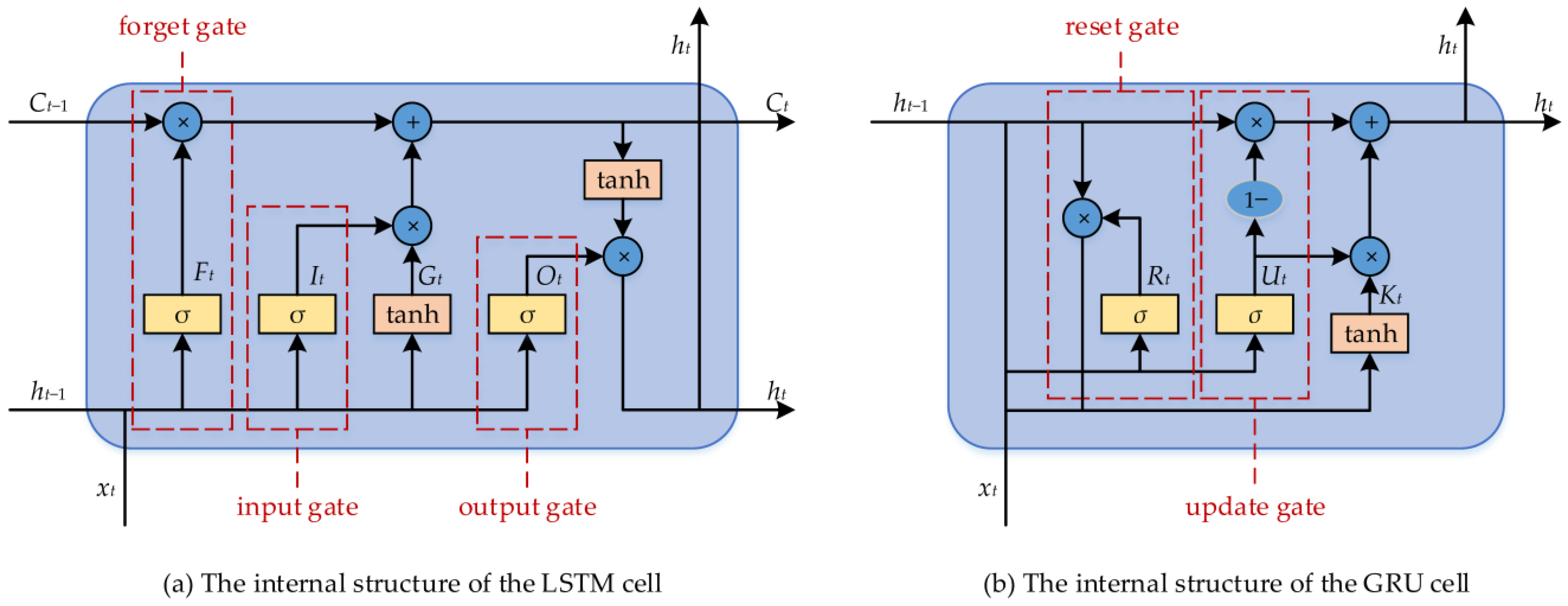
A schematic diagram of the internal structure of the LSTM is shown in Figure 1a; each gated memory unit consists of an input gate, an output gate and a forgetting gate in the internal structure of the LSTM. The input gate selectively updates new information to the current unit state, the forgetting gate selectively discards the information in the current unit state and the output gate selectively outputs the result [62]. The value of the current LSTM cell (ht) can be computed by the following equations.
where ht and ht-1 are, respectively, the outputs of the current and prior LSTM cells. Ft is the forgetting gate output of the current LSTM cell. It is the input gate output of the current LSTM cell. Ot is the output gate output of the current LSTM cell. Gt is the candidate state set of the current LSTM cell. Ct is the state of the current LSTM cell. xt is the input datum of the current LSTM cell. wFx, wIx, wGx, wOx, wFh, wIh, wGh and wOh are the weights of the current LSTM cell. bFx, bIx, bGx, bOx, bFh, bIh, bGh and bOh are the biases of the current LSTM cell. σ and tanh denote the sigmoid function and hyperbolic tangent function, respectively. ∗ denotes the Hadamard product.
The LSTM determines which units to suppress or activate based on the state of the previous unit, the currently stored state and the current input using gated memory units, which makes the LSTM more time-aware in time-series processing, means that it can learn when to forget and how long to retain state information, and allows the LSTM to remember information in longer time steps and have a better performance than the conventional RNN in processing long time-series data [63].
2.1.6. Gated Recurrent Unit
The GRU is an artificial neural network used to solve long-term dependencies in time series, which is a very efficient variant of the LSTM. The idea of the GRU is greatly similar to that of the LSTM. The LSTM uses an input gate, an output gate and a forgetting gate to design a gated memory unit to modulate the flow of information inside the neuron in the hidden layer, while the input gate and forgetting gate are combined into an update gate to balance previous activation and candidate activation in the GRU [11]. A schematic diagram of the internal structure of the GRU is shown in Figure 1b; each gated memory unit of the GRU mainly consists of an update gate and a reset gate. The update gate decides what information is discarded and what new information is added, and the reset gate decides what information is forgotten [64]. The value of the current GRU cell (ht) can be computed by the following equations.
where ht and ht-1 are, respectively, the outputs of the current and prior GRU cells. Rt is the reset gate output of the current GRU cell. Ut is the update gate output of the current GRU cell. Kt is the candidate set of the current GRU cell. xt is the input datum of the current GRU cell. wRx, wUx, wKx, wRh, wUh and wKh are the weights of the current GRU cell. bRx, bUx, bKx, bRh, bUh and bKh are the biases of the current GRU cell.
In the internal structure of the GRU cell, Rt and Ut are first obtained using Equations (8) and (9), respectively, based on the input data of the current GRU cell and the output of the prior GRU cell. Secondly, Kt is obtained using Equation (10) based on the input data and reset gate output of the current GRU cell and the output of the prior GRU cell. Lastly, ht is obtained using Equation (11) based on the update gate output and the candidate set of the current GRU cell and the output of the prior GRU cell [48]. It can be seen from Figure 1 that the GRU possesses a simpler structure compared to the LSTM. Consequently, it facilitates a faster training rate than the LSTM. Therefore, the GRU has been widely used in the field of artificial intelligence, especially in processing long time series.
2.2. Experimental Methods
2.2.1. Data Normalization
The input data of ML models may have different properties and different orders of magnitude, and model training without data normalization may diminish the impact of data of lower orders of magnitude. Therefore, the normalization of data is significant to improve the efficiency and performance of the ML model, and the data need to be normalized between 0 and 1 using the following equation before model training in this paper.
where yt is the normalized value of the data at time t; xt is the value of the original datum from the training dataset or the testing dataset at time t; and xmax and xmin are the maximum and minimum values of the original data from the training dataset, respectively.
2.2.2. Efficiency Criteria
After performing flood routing using the ML models, it is necessary to evaluate the performance of the ML models and analyze their accuracy and practicability. The most frequently used efficiency criteria, including the mean absolute percentage error (MAPE), the root mean square error (RMSE), the Nash–Sutcliffe efficiency coefficient (NSE), the correlation coefficient (R) and Kling–Gupta efficiency (KGE), are adopted to evaluate and compare the performance of different ML models during the training and testing periods in this paper. These efficiency criteria are defined as follows.
where Ot and St are, respectively, the observed and simulated values at time t; and are, respectively, the average values of the observed and simulated values; T is the number of Ot; and SDO and SDS are the standard deviations of the observed and simulated values, respectively. SDO and SDS can be respectively defined using the following equations.
2.2.3. Taylor Diagram
To describe visually the performance of different ML models, the Taylor diagram, which integrates the R, standard deviation (SD) and central root mean square error (CRMSE) in a single polar plot based on the cosine theorem, is introduced in this paper [65]. Combining the R, SD and CRMSE of the simulated values, the model performance can be represented as a dot by using the observed values as a reference dot in the Taylor diagram, and the relationship between these statistics can be defined using the following equation.
where CRMSE is the central root mean square error of the observed and simulated values, which can be also defined using the following equation.
Divide both sides of Equation (20) by the variance of the observed values at the same time, and Equation (22) can be obtained.
where NCRMSE and NSD are, respectively, the normalized CRMSE and the normalized SD, which can be respectively defined using the following equations.
The Taylor diagram can visually quantify the degree of correlation between the simulated and observed dots. The radial distance from the origin to the simulated dot characterizes the standard deviation of the simulation, and the orientation of the line connecting the origin and the simulated dot characterizes the correlation coefficient of the simulation. In the Taylor diagram, the closer the simulated dot of the model is to the observed dot, the better the model performance is. The Taylor skill score (TSS), which is a numerical summary of the Taylor diagram, can reflect a composite indicator of simulation skills and is defined using the following equation.
where R0 is the maximum correlation attainable and is identified as 0.9999 in this paper. For any given SDS, TSS increases monotonically with increasing R; for any given R, TSS increases as SDS approaches SDO. The larger the TSS of the model, the better the model performance is.
3. Case Study
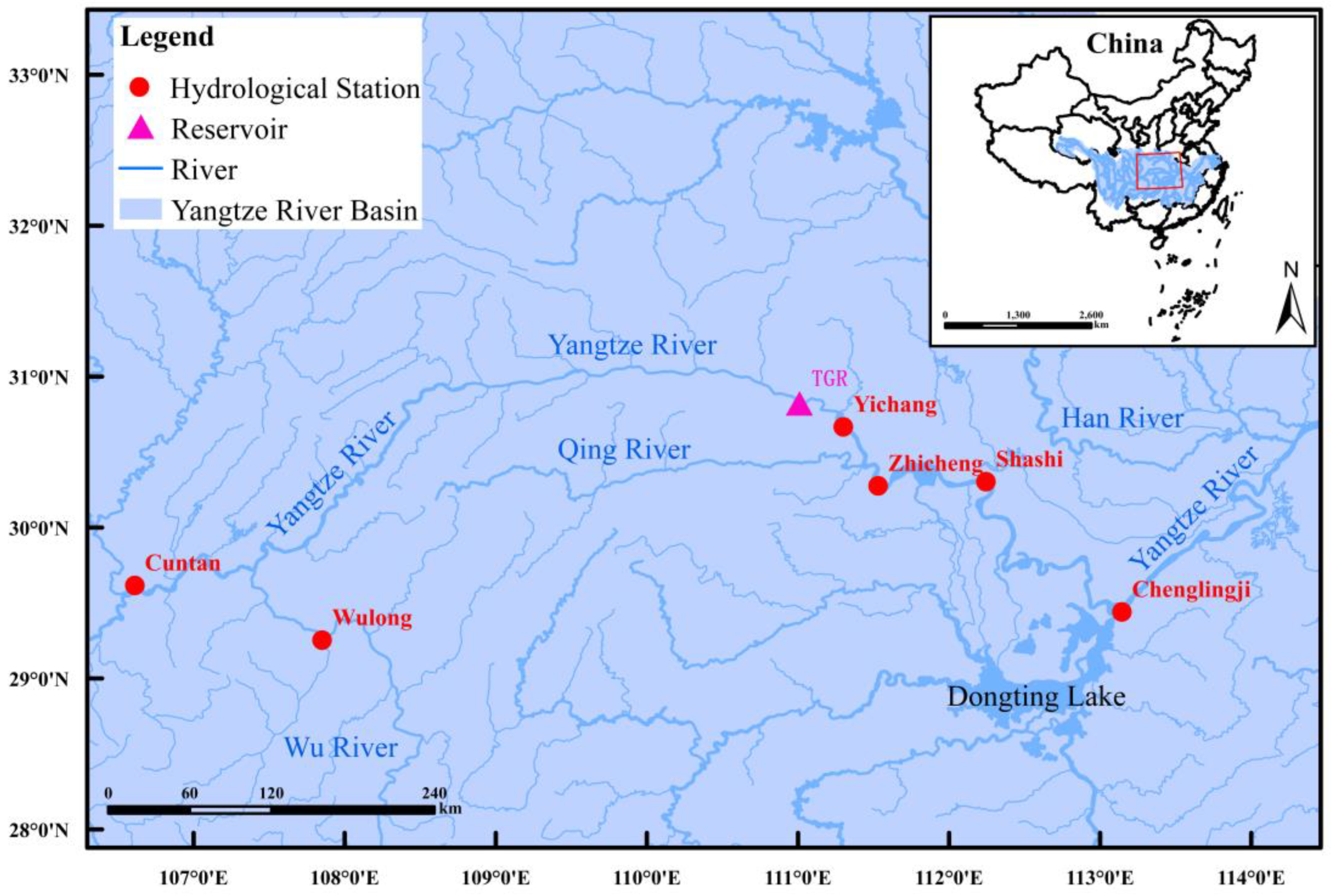
The Yangtze River spans three major regions in Southwest, Central and East China, with a total length of over 6300 km and a basin area of about 1.8 million km2, which makes it the third-largest river in the world and the first in China. Above Yichang are the upper reaches of the Yangtze River with a main stream length of over 4500 km and a drainage area of 1 million km2. From Yichang to Hukou are the middle reaches of the Yangtze River with a main stream length of over 950 km and a drainage area of 0.68 million km2. Below Hukou are the lower reaches of the Yangtze River with a main stream length of over 930 km and a drainage area of 0.12 million km2. In this paper, two reaches with complex water systems are selected as case studies to compare and analyze the applicability of different ML methods for flood routing in the Yangtze River. The first case study is a reach in the valley from Cuntan Station to the Three Georges Reservoir (TGR) with a main stream length of over 650 km, which is located at the end of the Upper Yangtze River and characterized by a long distance, a large river bottom drop, a deep canyon, rapid flow and many tributaries, which increases the difficulty of inflow forecasting of the TGR. A schematic diagram of the Yangtze River and hydrological stations is shown in Figure 2.
The second case study is a curved reach from Yichang Station to Shashi Station with a main stream length of over 140 km, which is located at the beginning of the Middle Yangtze River and has the characteristics of a curved channel, a wide river surface, a sharply reduced bottom drop, sluggish flow and a complex water system. The Jingjiang reach of the Yangtze River is from the Zhicheng Station to the Chenglingji Station. In the Jingjiang reach of the Yangtze River, part of the runoff flows southward into Dongting Lake through the Songzi River, the Hudu River and the Ouchi River, and then merges with the four rivers of Dongting Lake to join the Yangtze River again at Chenglingji Station, which causes a very complex water system in the Jingjiang reach and creates challenges in river flood routing.
The TGR is a key backbone project for the management and development of the Yangtze River, with comprehensive benefits of flood control, power generation, navigation, drought control, water supply, ecological environment, etc. The storage capacity provided by its huge flood control storage (22.15 billion m3) significantly enhances the flood control capacity of the Yangtze River in the Middle and Lower reaches, and the flood control standard of the downstream Jingjiang reach has risen from once every ten years to once every one hundred years. Cuntan Station and Wulong Station are the main control hydrological stations for the inflow hydrograph prediction of the TGR, and Zhicheng Station, Shashi Station and Chenglingji Station are the main flood control stations of the downstream Jingjiang reach. Therefore, the inflow hydrograph prediction of the TGR and the water level hydrograph prediction of Shashi Station for flood routing in the Yangtze River are scientific problems with important academic significance and engineering application value, which play an important role in guaranteeing the flood control security of the Jingjiang reach of the Yangtze River as well as China’s energy security.
The daily average discharge series of Cuntan Station, Wulong Station and Yichang Station, the daily average inflow series of the TGR, and the daily average water level series of Zhicheng Station and Shashi Station from 1 January 1996 to 31 October 2020 are collected in this study. The drainage area above the Three Gorges dam is about 1 million km2, and the drainage areas above Cuntan Station and Wulong Station are about 867,000 and 88,000 km2, respectively. The drainage areas above Yichang Station, Zhicheng Station and Shashi Station are over 1.0055, 1.0241 and 1.0320 million km2, respectively. According to the location relationship between these stations, the daily average discharge series of Cuntan Station and Wulong Station are used for inflow prediction of the TGR so as to consider the influence of the discharge from the Wu River, and the daily average discharge series of Yichang Station and the daily average water level series of Zhicheng Station are used for water level prediction of Shashi Station so as to consider the influence of the discharge from the Qing River.
4. Results and Discussion
4.1. Experimental Conditions
The daily average discharge series and the daily average water level series of hydrological stations from 1 January 1996 to 31 October 2020 were divided into two parts, which were used as the training dataset (from 1 January 1996 to 13 November 2015) and the testing dataset (from 14 November 2015 to 31 October 2020). Thus, a total of 7257 days of daily average discharge or water levels of hydrological stations from 1996 to 2015 were used to train the models, and a total of 1814 days of daily average discharge or water levels of hydrological stations from 2015 to 2020 were used to verify the models. Fortunately, the maximum and minimum values of the historical observation data were divided in the training dataset for these two case studies. The training dataset and the testing dataset were both normalized between 0 and 1, adopting the method described above.
In this paper, the SVR, GPR and RFR models were implemented in the Python programming language using the “scikit-learn” package, while the MLP, LSTM and GRU models were implemented in the Python programming language using the “keras” package. The hyper-parameters of six ML models were chosen by a manual trial-and-error method based on referring to relevant references. For the SVR model, the penalty parameter was 1.0, the slack variable was 0.1 and the kernel function was the linear kernel. For the GPR model, the kernel function was the radial basis function kernel with a length scale of 10. For the RFR model, the number of trees was 300, the maximum depth of the tree was 7 and the number of features was 9. For the MLP model, the number of hidden layers was 1, and the number of neurons in the hidden layer was 100. For the LSTM model, the number of hidden layers was 1, and the number of neurons was 100. For the GRU model, the number of hidden layers was 1, and the number of neurons was 100. The models were first trained using the training dataset, and then the trained ML models were used to predict the inflow hydrograph of the TGR and the water level hydrograph of Shashi Station. After that, the performances of the six ML models for flood routing in the Yangtze River were analyzed and discussed.
4.2. The Inflow Hydrograph Prediction of the TGR
The large tributaries involved in the section from Cuntan Station to the TGR are mainly those of the Wu River, and the daily average discharge series of Cuntan Station and Wulong Station, which is the main control hydrological station in the lower reaches of the Wu River, are necessary to predict the inflow hydrograph of the TGR. The correlation analysis and the experiment showed that the daily average discharge series data of Cuntan Station and Wulong Station in the 7 days before are most helpful to predict the current inflow series of the TGR. Thus, the models were respectively executed to predict the inflow hydrograph of the TGR using the daily average discharge series of Cuntan Station and Wulong Station in the 7 days before. Taking the calculation of the inflow of the TGR at day t as an example, the input data of the models included the average discharge of Cuntan Station and Wulong Station from day t−6 to day t and the inflow of TGR from day t−7 to day t−1.
To compare the performance of the ML models with the conventional river flood routing model, the linear Muskingum model (LMM), which has been used in flood routing for the main stream of the Yangtze River, was used to implement the flood routing for the river from Cuntan Station to the TGR. The LMM has been extensively described in relevant references [66], and its parameters are optimized by the original genetic algorithm with the objective of minimizing the sum of the squared deviations between observed and simulated values. The efficiency criteria of the models during the training and testing period are shown in Table 1. The RFR model had better efficiency criteria than other models during the training period, while it did not perform as well during the testing period, which indicates that the RFR model is likely to have overfitting for inflow hydrograph prediction of the TGR. Conversely, the GRU model had a poor performance compared with the RFR model during the training period, but the efficiency criteria of the GRU model outperformed those of the other models, except for R, during the testing period. In particular, compared to other ML models, the reductions in the MAPE and RMSE by the GRU model were at least 7.66% and 3.80% during the testing period, respectively. With the exception of the SVR model, the LMM had the worst performance during the testing period, and the reductions in the MAPE and RMSE by the GRU model were 29.32% and 26.17% compared to the LMM during the testing period, respectively. In addition, the training times of the LSTM and GRU are longer than those of other models, and the training time of the GRU is shorter than that of the LSTM, which indicates that the model with higher accuracy may also require a longer training time, but the GRU has a faster training rate than the LSTM.
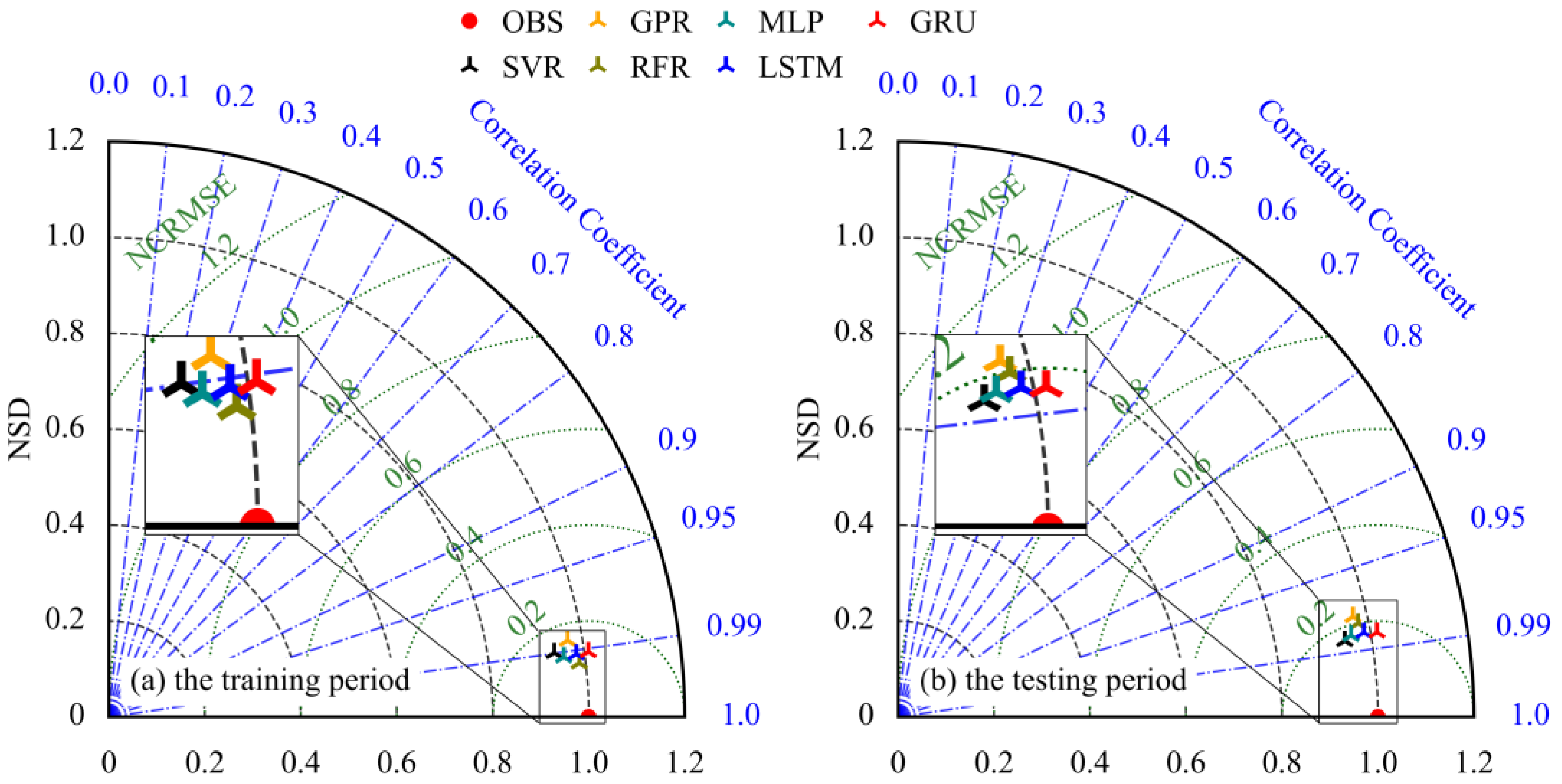
As a consequence, the Taylor diagram and the TSSs are necessary to visualize the performance of the ML models. A Taylor diagram depicting the performance of six ML models for inflow hydrograph prediction of the TGR is shown in Figure 3.
Clearly, the simulated dot of the RFR model is closer to the observed dot than those of other models during the training period, but it is not the closest dot to the observed dot during the testing period. Therefore, it can also reach a decision from the Taylor diagram that there is an overfitting problem for the inflow hydrograph prediction of the TGR by the RFR model. In addition, the simulated dot of the GRU model was closer to the observed dot than other models during the testing period, and the GRU model had a better performance than the SVR model in terms of the efficiency criteria of the models, even though the correlation coefficient of the SVR model was better than that of the GRU model. Furthermore, the TSS of the GRU model was greater than that of the SVR model during the testing period (as can be seen in Table 1), which also indicated that the GRU model outperformed the other models for inflow hydrograph prediction of the TGR.
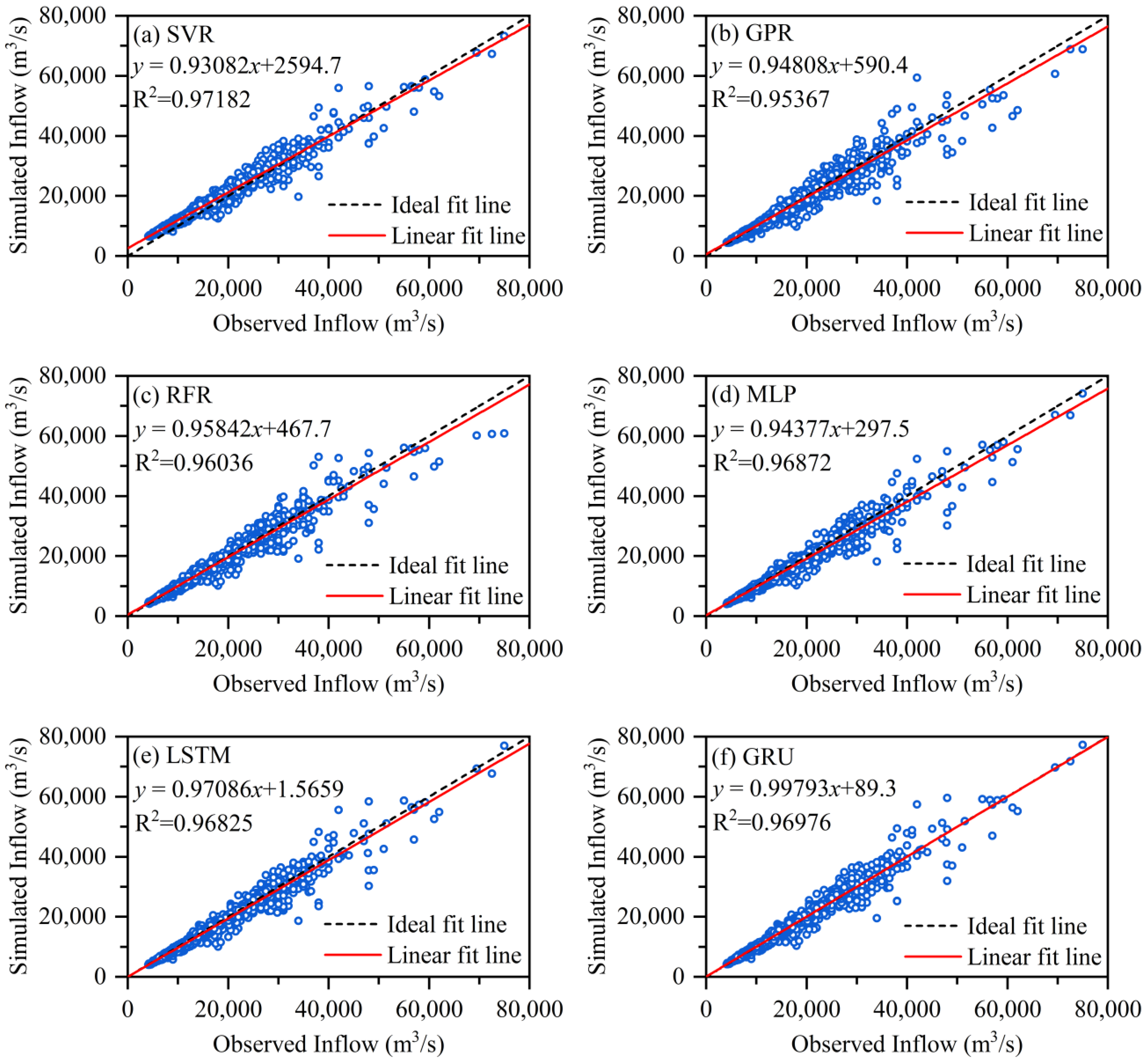
While the efficiency criteria of the models can assess the overall performance of the ML models, scatter plots and boxplots can be used to further analyze the simulation errors of the ML models and reveal additional and more specific information. The scatter plots of the simulated and observed inflows of the TGR by different ML models during the testing period are shown in Figure 4.
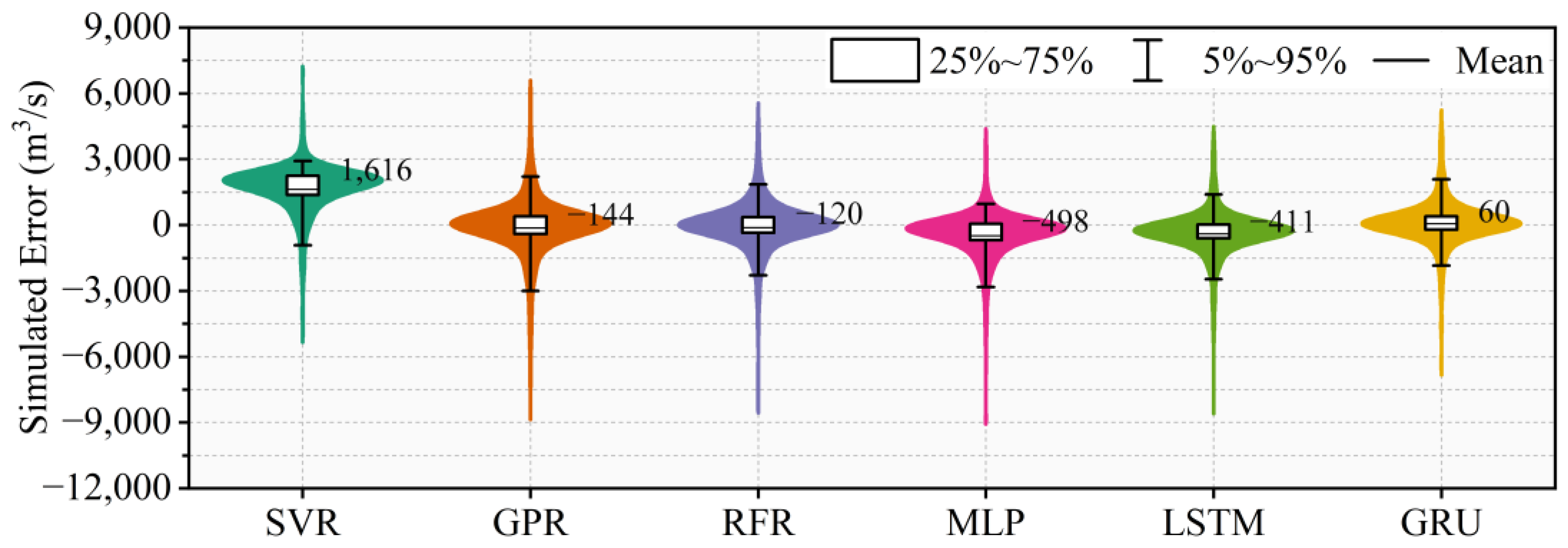
The linear fit equation between the simulated inflows by the ML model and observed inflows of the TGR is given in Figure 4, and the R2 characterizes the accuracy of the linear fit equation. The larger the R2 is, the more the data points are concentrated on both sides of the linear fit line. The closer the slope of the linear fit line is to 1 and the closer the intercept is to 0, the better the linear fit line matches the ideal fit line, and the better the simulated inflows and the observed inflows of the TGR are matched. Therefore, the slope of the linear fit line of the GRU model is closest to 1, and the linear fit line of the GRU model is more in line with the ideal fit line than those of the other ML models, which means that the simulated inflows of the TGR of the GRU model are closest to the corresponding observed inflows. In order to analyze the distribution pattern of the simulated inflow errors of the TGR of the different ML models, violin plots of the simulated inflow errors by different ML models during the testing period are shown in Figure 5.
As can be seen in Figure 5, the means of the simulated errors of the SVR and GRU models are both positive numbers, while the ones of the GPR, RFR, MLP and LSTM models are all negative numbers, which means that the simulated inflows of the SVR and GRU models are roughly larger than the observed inflows of the TGR, while the opposite is the case for the GPR, RFR, MLP and LSTM models. In general, the closer the mean of simulated inflow errors is to 0, the better the water balance can be ensured when performing flood routing, which is also an important indicator for river flood routing. In consequence, the inflow hydrograph prediction of the TGR using the GRU model guarantees a better water balance. It is also reaffirmed that the GRU model exhibits a stronger performance than the other ML models for simulating the inflow hydrograph of the TGR.
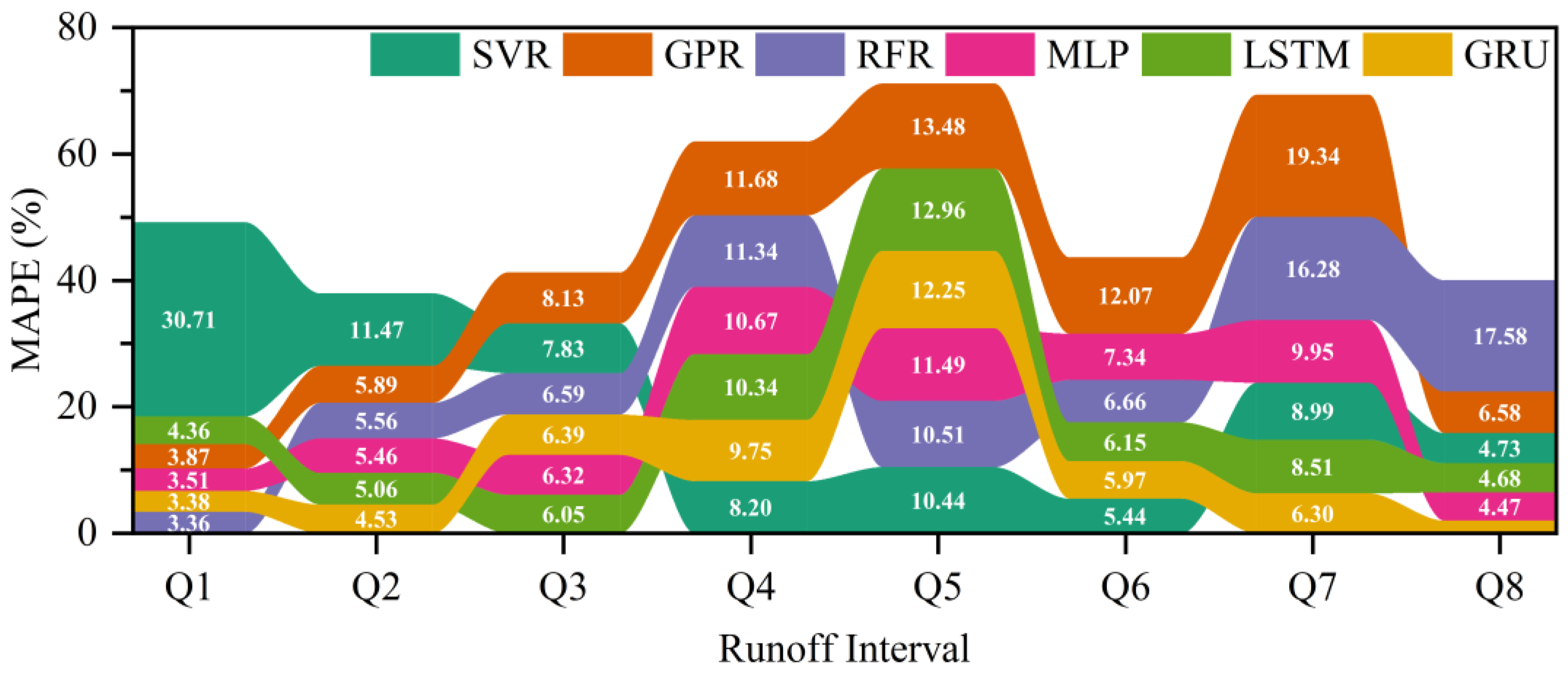
In order to evaluate the accuracy of the models for different sizes of discharge, the inflow of the TGR was divided into eight discharge intervals, namely, Q1 (not greater than 10,000 m3/s), Q2 (from 10,000 to 20,000 m3/s), Q3 (from 20,000 to 30,000 m3/s), Q4 (from 30,000 to 40,000 m3/s), Q5 (from 40,000 to 50,000 m3/s), Q6 (from 50,000 to 60,000 m3/s), Q7 (from 60,000 to 70,000 m3/s) and Q8 (greater than 70,000 m3/s), and the ribbon diagram of the MAPEs for inflow hydrograph prediction of the TGR by the models during the testing period is shown in Figure 6. For the inflow of the TGR from 30,000 to 50,000 m3/s, namely, discharge interval Q4 and Q5, all models had a larger MAPE, around 10%. The GPR and RFR models had relatively poor MAPEs for larger inflow, the SVR model had a poor MAPE for a smaller inflow, and the MLP, LSTM and GRU models had relatively better MAPEs for smaller and larger inflows. Overall, the GRU model had a smaller MAPE.
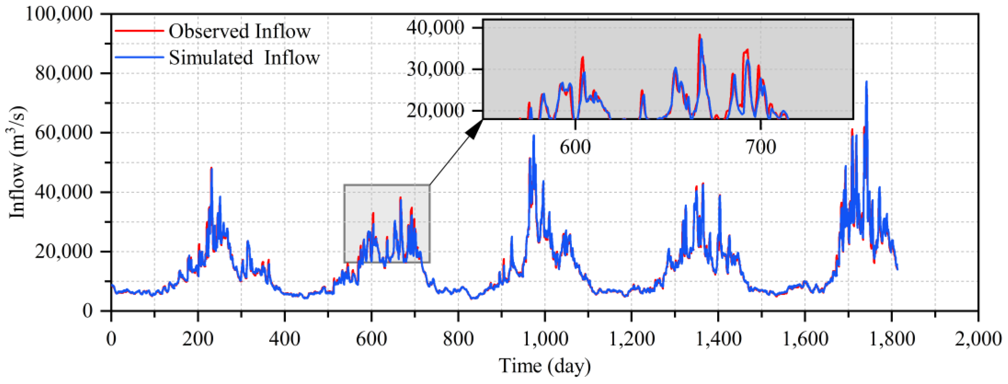
The simulated inflow hydrograph of the TGR by the GRU during the testing period is shown in Figure 7. It can be seen that the simulated inflow hydrograph of the TGR by the GRU model is basically consistent with the observed inflow hydrograph but does not fit well with the observed inflow in some cases (such as from day 570 to 720). Nevertheless, the GRU model had a better performance than the other models and is the most suitable model for flood routing of the river from Cuntan Station to the TGR considering the influence of the Wu River.
4.3. The Water Level Hydrograph Prediction of Shashi Station
The large tributaries involved in the section from Yichang Station to Shashi Station are mainly those of the Qing River, and the daily average discharge series of Yichang Station and the daily water level series of Zhicheng Station, which are used to consider the impact of the Qing River on the water level hydrograph prediction of Shashi Station, are necessary to predict the water level hydrograph of Shashi Station. The correlation analysis and the experiment showed that the daily average discharge or water level series of the Yichang and Zhicheng Stations in the 3 days before are most helpful in predicting the current water level series of Shashi Station. To further compare and analyze the effectiveness of the models for flood routing in the Yangtze River, the models were respectively modeled to predict the water level hydrograph of Shashi Station using the first three days of daily average discharge or water level series of Yichang Station and Zhicheng Station. Taking the calculation of the water level of Shashi Station at day t as an example, the input data of the models included the average discharge of Yichang Station from day t−2 to day t, the average water level of Zhicheng Station from day t−2 to day t and the average water level of Shashi Station from day t−3 to day t−1. The efficiency criteria of the models for water level hydrograph prediction of Shashi Station during the training and testing period are shown in Table 2.
It is apparent from Table 2 that the MLP and GRU models have the same MAPE, RMSE and NSE values, and are better than other ML models, whereas the R and TSS values of the MLP model are slightly smaller than the ones of the GRU model in the training period. Moreover, the GRU model has the best efficiency criteria during the testing period. Specifically, compared to other ML models, the GRU model reduced the MAPE and RMSE by at least 19.51% and 11.76% during the testing period, respectively. The GRU model had no worse efficiency criteria than other ML models during the training period and it performed as well during the testing period, which indicates that the GRU model can learn the relationship between the upstream stations and the downstream station. Furthermore, the training time of the GRU is 26.14% shorter than the one of the LSTM, which ties in with the available relevant research conclusion that the training speed of GRU is also faster than that of LSTM [67,68]. Therefore, Table 2 demonstrate that the GRU model is a better model for the water level hydrograph prediction of Shashi Station in flood routing.
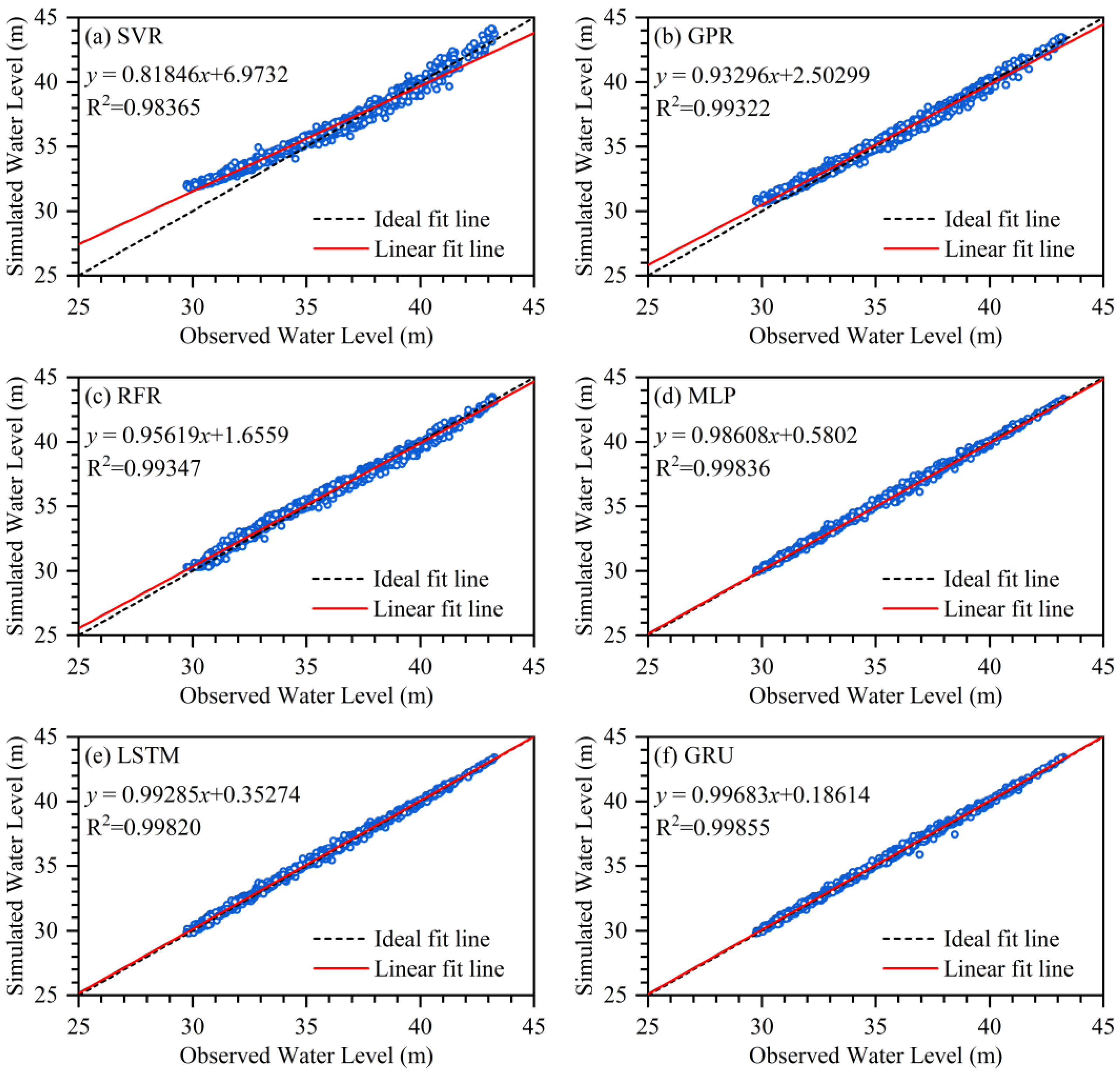
The scatter plots of the simulated and observed water levels of Shashi Station by different ML models during the testing period are shown in Figure 8. Obviously, the linear fit line by the MLP, LSTM and GRU models is more in line with the ideal fit line than the ones of the SVR, GPR and RFR models.
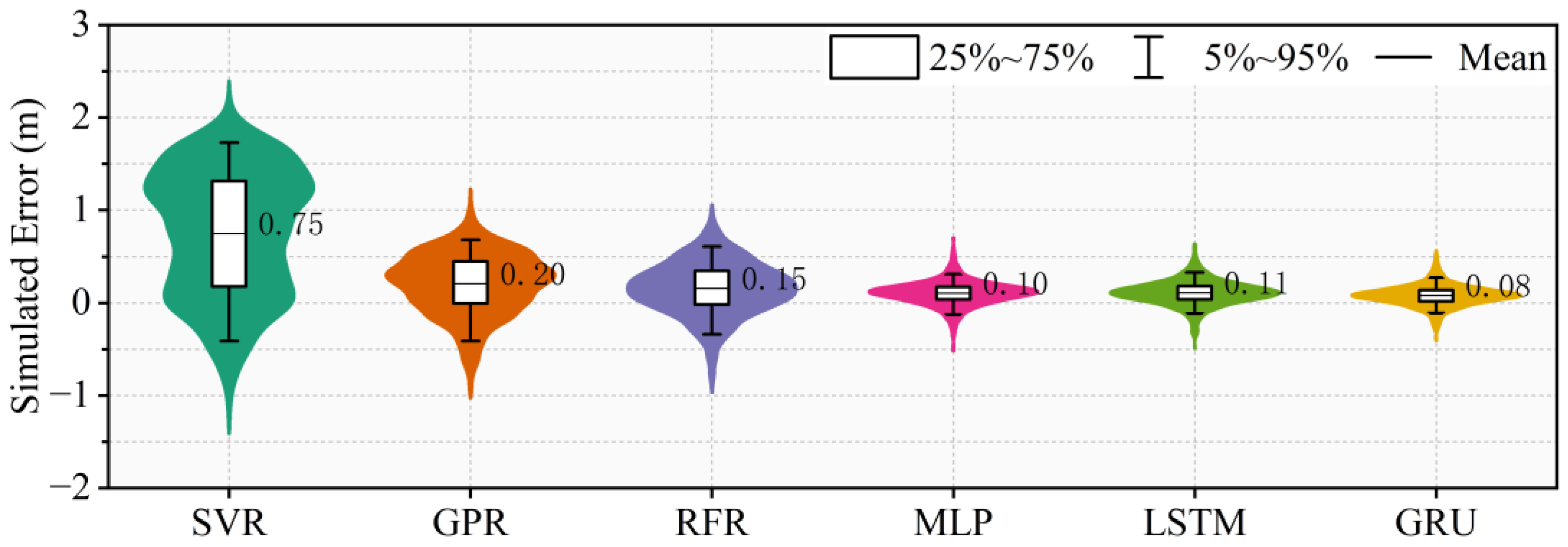
Violin plots of the simulated water level errors of Shashi Station during the testing period are shown in Figure 9 to illustrate the distribution pattern of the simulated water level errors of different ML models. It can easily be seen that the simulated water level errors of Shashi Station by the MLP, LSTM and GRU models are relatively close and much smaller than those of the SVR, GPR and RFR models on the whole. Furthermore, the mean of the simulated water level errors of the GRU model is the closest to 0, and the water level hydrograph prediction of Shashi Station using the GRU model guarantees a better water balance than the other ML models. Therefore, the same conclusion as in the previous section can be drawn that the GRU model exhibits a stronger performance than the other ML models for simulating the water level hydrograph of Shashi Station.
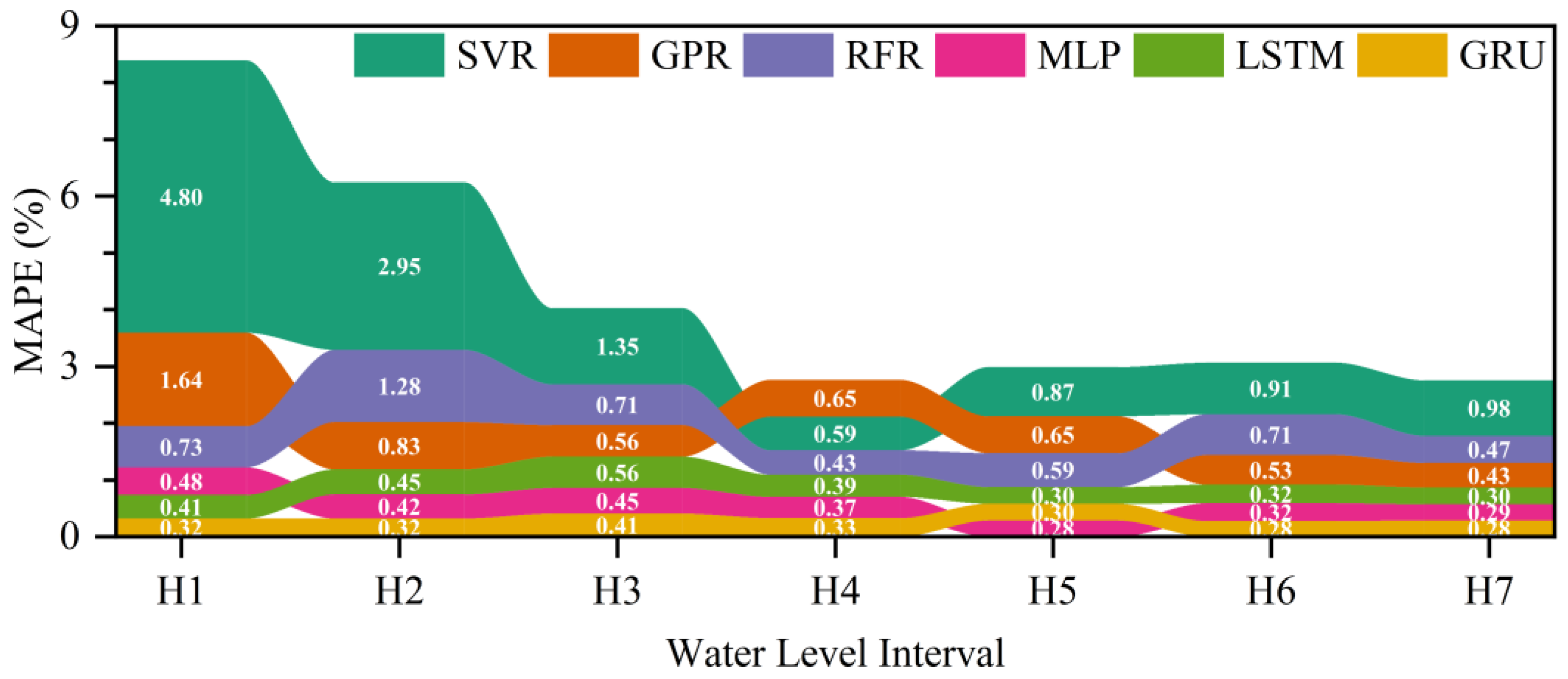
In order to evaluate the accuracy of the models for different water levels during the testing period, the water level of Shashi Station was divided into seven water level intervals, namely, H1 (not greater than 32 m), H2 (from 32 to 34 m), H3 (from 34 to 36 m), H4 (from 36 to 38 m), H5 (from 38 to 40 m), H6 (from 40 to 42 m) and H7 (greater than 42 m), and the ribbon diagram of the MAPEs for water level hydrograph prediction of Shashi Station by the models during the testing period is shown in Figure 10. The SVR, GPR and RFR models have poorer MAPEs than the MLP, LSTM and GRU models, and the GRU model had the smallest MAPE except for the water level interval H5, namely, for the water level of Shashi Station from 38 to 40 m. As a consequence, the GRU model is superior to the other models.
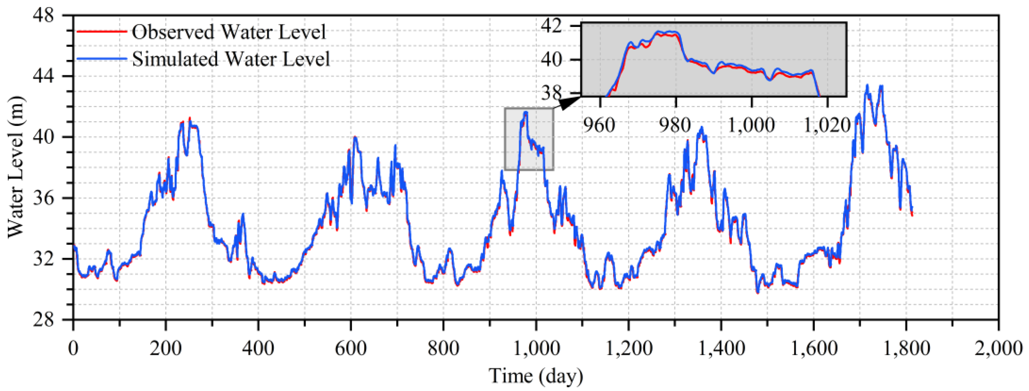
The simulated water level hydrograph of Shashi Station by the GRU during the testing period is shown in Figure 11. The simulated water level hydrograph by the GRU model is almost consistent with the observed water level hydrograph but does not simulate the water level hydrograph of Shashi Station very well in some cases (for instance, the simulated water level hydrograph from day 960 to 1020 is roughly above the observed water level hydrograph). On the whole, the GRU model is also the most suitable model for flood routing in the river from Yichang Station to Shashi Station considering the influence of the Qing River.
According to the results of two case studies in the Yangtze River, the deep learning models, such as the MLP, LSTM and GRU, seem to be more effective than the other ML models. The simulated values of the MLP, LSTM and GRU models are closer than those of the SVR, GPR and RFR models to the corresponding observed values (see Figure 4 and Figure 8), and the simulated errors of the MLP, LSTM and GRU models are relatively smaller than those of the SVR, GPR and RFR models on the whole (see Figure 5 and Figure 9). Deep learning models can automatically learn more effective sample features than traditional ML models, which makes them better at handling high-dimensional and nonlinear problems, and deep learning models have better generalization abilities and usually perform well on both training and testing datasets.
For river flood routing, the discharge or water level of the hydrological station has an apparent long-term dependency on its previous discharge or water level and those of upstream hydrological stations, and the LSTM and GRU models are appropriate for solving this type of prediction problem because both the GRU and LSTM models can effectively suppress gradient disappearance or explosion due to long-term dependence [27]. Nevertheless, the results of this paper indicate that the GRU model can obtain better forecasting performance with fewer parameters and shorter training times compared with the complex computation and slow training speed of the LSTM model, which is consistent with the other available relevant research conclusions [33,69,70]. Therefore, the GRU model has a simpler structure and converges more easily during the training period, which allows the model to better capture long-term dependencies and perform better generalizations on fewer samples for the prediction problem of nonlinear, non-smooth and strongly fluctuating time-series data [10].
Of special note is that the GRU model performs well in predicting almost all different extents of water levels of the Shashi Station; however, it has poor performance in predicting the inflows of the TGR, particularly for inflows from 30,000 to 50,000 m3/s (the obtained MAPE is around 10%), which may be related to the long distance from Cuntan Station to the TGR and the influence of many small tributaries with no observation data for this river.
4.4. Performance Comparison among Three Deep Learning Models with Different Time Lags for Flood Routing
It is worth noting that the above conclusions were obtained with the determination of the appropriate time lags for flood routing. In general, the larger the time lag, the more input variables the deep learning model has, and the better the generalization ability of the model, which leads to a higher performance. However, more input variables may also cause the model to be more difficult to train, resulting in the model not finding the optimal parameters, which in turn may affect the performance of the model. In addition, the time lags for flood routing depends to a large extent on the propagation time of the flood waves over the river, but they may not be exactly numerically equal, because the propagation time of flood waves over the river may not be an exact integer number of days. Therefore, it is important to determine the appropriate time lag in addition to selecting the appropriate ML model based on the characteristics of the study area when using an ML model for flood routing, and the appropriate time lags for flood routing in the two case studies presented in this paper were 7 days and 3 days, respectively.
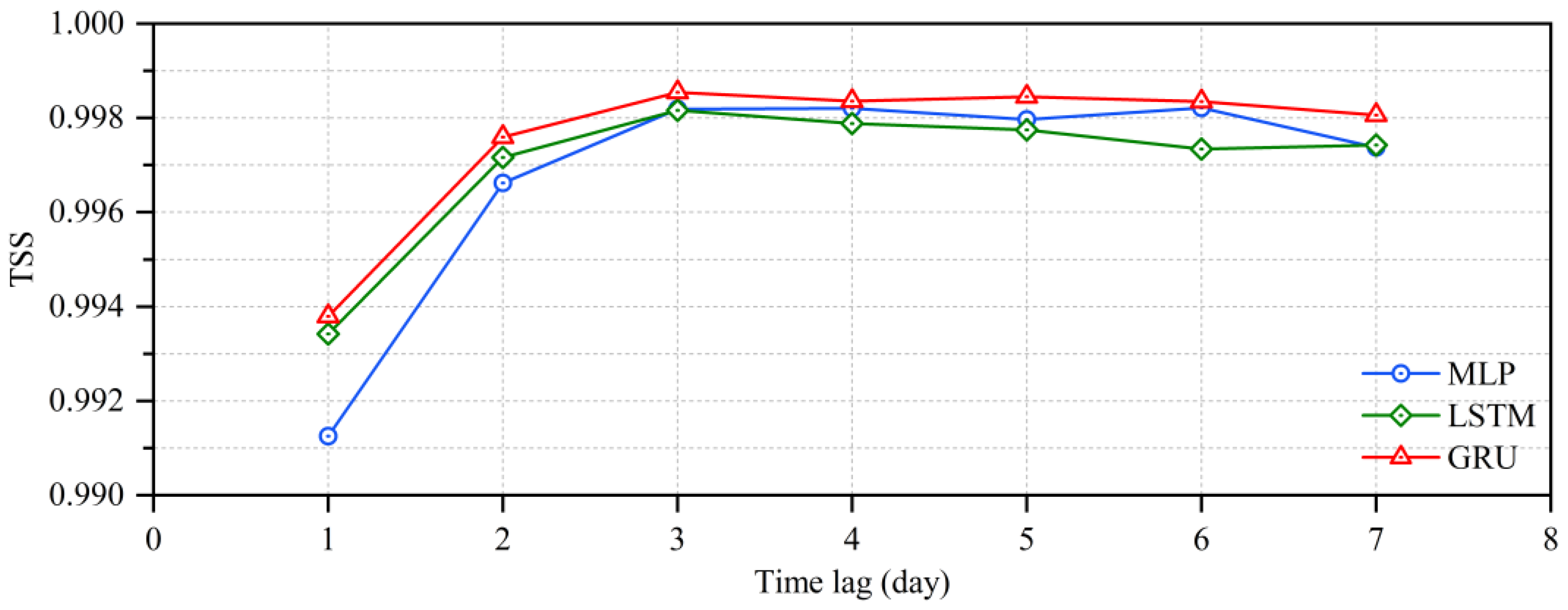
To further compare and analyze the performance of three deep learning models with different time lags for flood routing, taking the flood routing from Yichang Station to Shashi Station as an example, the MLP, LSTM and GRU models with different time lags for water level hydrograph prediction of Shashi Station were respectively trained, and the TSSs of the MLP, LSTM and GRU models during the testing period are shown in Figure 12. It is apparent that the TSS obtained by the GRU model is larger than the ones obtained by the MLP and LSTM models for different time lags, which indicates that the GRU is more suitable than the MLP and LSTM for flood routing in the river from Yichang Station to Shashi Station, considering the influence of the Qing River. Furthermore, the TSSs obtained by the MLP, LSTM and GRU models all gradually increased and then slightly decreased as the time lag increased during the testing period, and the TSSs obtained by the MLP, LSTM and GRU models reached maximum values when the lag time was 3 days, which is the reason why the first three days of the daily average discharge series of Yichang Station and the first three days of the daily average water level series of Zhicheng Station were used to predict the water level hydrograph of Shashi Station in the previous section.
Therefore, the ML model is a nice choice for flood routing in complex natural rivers that do not have abundant topographic measurements available, and the GRU model exhibits a better performance for flood routing in the Yangtze River than other comparative ML models. In addition, it is important to determine the appropriate time lag as well as select the appropriate model based on the characteristics of the study area when using an ML model for flood routing.
5. Conclusions
It is important to obtain more accurate flood information downstream of a reservoir for guiding reservoir regulation and reducing flood disasters. In this work, the popular ML models, including the SVR, GPR, RFR, MLP, LSTM and GRU models, were selected and applied to the flood routing of two complicated reaches in the Yangtze River. The first reach was located at the end of the Upper Yangtze River and characterized by a long distance, a large river bottom drop, a deep canyon, rapid flow and many tributaries, and the second reach was located at the beginning of the Middle Yangtze River and had the characteristics of a curved channel, a wide river surface, a sharply reduced bottom drop, sluggish flow and a complex water system. These unique features pose challenges in river flood routing and make it difficult to create accurate physical models. A total of 7257 days of daily average discharge or water levels of hydrological stations from 1996 to 2015 were first used to train the models, and then a total of 1814 days of daily average discharge or water levels of hydrological stations from 2015 to 2020 were used to verify the effectiveness of the models for flood routing. According to the results obtained from various models, some conclusions could be drawn and can be summarized as follows:
- (1)
- The ML models were verified as effective and efficient in obtaining accurate flood hydrographs in river flood routing with fewer data (e.g., only flows and water levels that are daily measured). Therefore, the ML models could be widely used for flood routing in complex natural rivers. However, it is important to note that not all ML models were equally effective in flood routing, as some may overfit during the training phase.
- (2)
- The deep learning models, including the MLP, LSTM and GRU models, were more efficient than the SVR, GPR and RFR models. The GRU model, in particular, outperformed the others in almost all efficiency criteria, including MAPE, RMSE, NSE, TSS and KGE. The reductions in MAPE and RMSE were significant, with at least 7.66% and 3.80% for the first case study and 19.51% and 11.76% for the second case study during the testing period.
- (3)
- The model that had higher accuracy may necessitate a longer training time, but the GRU exhibited a faster training rate than the LSTM. Although the training times of the LSTM and GRU were longer than those of the other models, the GRU’s training times were, respectively, 32.19% and 26.14% shorter than those of the LSTM for the two case studies due to its simpler structure and more effortless convergence.
- (4)
- The time lag in flood routing determined the number of input variables of the models, which in turn may have affected the accuracy of flood routing. As a result, the accuracy of flood routing gradually increased and then slightly decreased as the time lag increased for the MLP, LSTM and GRU models. Interestingly, the GRU model performed better than the MLP and LSTM models for different time lags.
This paper has yielded some valuable research findings; however, there are some limitations that require further in-depth investigation in the future. The hyper-parameters of models should be optimized by the optimization algorithm with intelligent performance, and the sensitivities of these hyper-parameters with respect to the results should be studied, which could perhaps lead to further improvement of the performance of the model. In the near future, the decomposition method could be combined and hybrid models could be studied by taking advantage of different models to realize river flood routing and further improve the accuracy of river flood routing. Moreover, utilizing discharge or water level data with higher frequencies, such as hourly averages, for flood routing may further determine more appropriate time lags and thus improve the accuracy of the model, and could also facilitate flood routing for smaller rivers that experience flood events lasting less than a day, if data with higher frequencies are available. Furthermore, the main uncertainty resources in this paper may encompass the hydrological characteristics of the selected study area, the potential bias in the model training samples, the omission of precipitation uncertainty, the limited model selection, and so on, which may have influenced the research findings to some degree and warrant further investigation.
Author Contributions
Conceptualization, L.Z. and L.K.; Methodology, L.Z.; Software, L.Z.; Validation, L.Z. and L.K.; Formal analysis, L.Z. and L.K.; Investigation, L.Z.; Resources, L.K.; Data curation, L.Z.; Writing—original draft preparation, L.Z.; Writing—review and editing, L.K.; Visualization, L.Z.; Supervision, L.K.; Project administration, L.K.; Funding acquisition, L.K. All authors have read and agreed to the published version of the manuscript.
Funding
This research was funded by the National Key R&D Program of China (grant nos. 2021YFC3200302 and 2022YFC3002704).
Institutional Review Board Statement
Not applicable.
Informed Consent Statement
Not applicable.
Data Availability Statement
Not applicable.
Conflicts of Interest
The authors declare no conflict of interest.
References
- Akbari, R.; Hessami-Kermani, M.R.; Shojaee, S. Flood Routing: Improving Outflow Using a New Non-linear Muskingum Model with Four Variable Parameters Coupled with PSO-GA Algorithm. Water Resour. Manag. 2020, 34, 3291–3316. [Google Scholar] [CrossRef]
- Kang, L.; Zhou, L.; Zhang, S. Parameter Estimation of Two Improved Nonlinear Muskingum Models Considering the Lateral Flow Using a Hybrid Algorithm. Water Resour. Manag. 2017, 31, 4449–4467. [Google Scholar] [CrossRef]
- Zhang, S.; Kang, L.; Zhou, L.; Guo, X. A new modified nonlinear Muskingum model and its parameter estimation using the adaptive genetic algorithm. Hydrol. Res. 2017, 48, 17–27. [Google Scholar] [CrossRef]
- Yuan, X.; Wu, X.; Tian, H.; Yuan, Y.; Adnan, R.M. Parameter Identification of Nonlinear Muskingum Model with Backtracking Search Algorithm. Water Resour. Manag. 2016, 30, 2767–2783. [Google Scholar] [CrossRef]
- Kim, D.H.; Georgakakos, A.P. Hydrologic routing using nonlinear cascaded reservoirs. Water Resour. Res. 2014, 50, 7000–7019. [Google Scholar] [CrossRef]
- Jeng, R.I.; Coon, G.C. True Form of Instantaneous Unit Hydrograph of Linear Reservoirs. J. Irrig. Drain. Eng. 2003, 129, 11–17. [Google Scholar] [CrossRef]
- Dhote, P.R.; Thakur, P.K.; Domeneghetti, A.; Chouksey, A.; Garg, V.; Aggarwal, S.P.; Chauhan, P. The use of SARAL/AltiKa altimeter measurements for multi-site hydrodynamic model validation and rating curves estimation: An application to Brahmaputra River. Adv. Space Res. 2021, 68, 691–702. [Google Scholar] [CrossRef]
- Singh, R.K.; Kumar Villuri, V.G.; Pasupuleti, S.; Nune, R. Hydrodynamic modeling for identifying flood vulnerability zones in lower Damodar river of eastern India. Ain Shams Eng. J. 2020, 11, 1035–1046. [Google Scholar] [CrossRef]
- Chatterjee, C.; Förster, S.; Bronstert, A. Comparison of hydrodynamic models of different complexities to model floods with emergency storage areas. Hydrol. Process. 2008, 22, 4695–4709. [Google Scholar] [CrossRef]
- Cho, M.; Kim, C.; Jung, K.; Jung, H. Water Level Prediction Model Applying a Long Short-Term Memory (LSTM)-Gated Recurrent Unit (GRU) Method for Flood Prediction. Water 2022, 14, 2221. [Google Scholar] [CrossRef]
- Jeong, J.; Park, E. Comparative applications of data-driven models representing water table fluctuations. J. Hydrol. 2019, 572, 261–273. [Google Scholar] [CrossRef]
- Zhang, Z.; Zhang, Q.; Singh, V.P. Univariate streamflow forecasting using commonly used data-driven models: Literature review and case study. Hydrol. Sci. J. 2018, 63, 1091–1111. [Google Scholar] [CrossRef]
- Niu, W.J.; Feng, Z.K.; Feng, B.F.; Min, Y.W.; Cheng, C.T.; Zhou, J.Z. Comparison of Multiple Linear Regression, Artificial Neural Network, Extreme Learning Machine, and Support Vector Machine in Deriving Operation Rule of Hydropower Reservoir. Water 2019, 11, 17. [Google Scholar] [CrossRef] [Green Version]
- Zhang, J.; Xiao, H.; Fang, H. Component-based Reconstruction Prediction of Runoff at Multi-time Scales in the Source Area of the Yellow River Based on the ARMA Model. Water Resour. Manag. 2022, 36, 433–448. [Google Scholar] [CrossRef]
- Yan, B.; Mu, R.; Guo, J.; Liu, Y.; Tang, J.; Wang, H. Flood risk analysis of reservoirs based on full-series ARIMA model under climate change. J. Hydrol. 2022, 610, 127979. [Google Scholar] [CrossRef]
- Lian, Y.; Luo, J.; Xue, W.; Zuo, G.; Zhang, S. Cause-driven Streamflow Forecasting Framework Based on Linear Correlation Reconstruction and Long Short-term Memory. Water Resour. Manag. 2022, 36, 1661–1678. [Google Scholar] [CrossRef]
- Ebrahimi, E.; Shourian, M. River Flow Prediction Using Dynamic Method for Selecting and Prioritizing K-Nearest Neighbors Based on Data Features. J. Hydrol. Eng. 2020, 25, 04020010. [Google Scholar] [CrossRef]
- Dehghani, R.; Babaali, H.; Zeydalinejad, N. Evaluation of statistical models and modern hybrid artificial intelligence in the simulation of precipitation runoff process. Sustain. Water Resour. Manag. 2022, 8, 154. [Google Scholar] [CrossRef]
- Rahbar, A.; Mirarabi, A.; Nakhaei, M.; Talkhabi, M.; Jamali, M. A Comparative Analysis of Data-Driven Models (SVR, ANFIS, and ANNs) for Daily Karst Spring Discharge Prediction. Water Resour. Manag. 2022, 36, 589–609. [Google Scholar] [CrossRef]
- Yaseen, Z.M.; Sulaiman, S.O.; Deo, R.C.; Chau, K.-W. An enhanced extreme learning machine model for river flow forecasting: State-of-the-art, practical applications in water resource engineering area and future research direction. J. Hydrol. 2019, 569, 387–408. [Google Scholar] [CrossRef]
- Zhu, S.; Luo, X.; Xu, Z.; Ye, L. Seasonal streamflow forecasts using mixture-kernel GPR and advanced methods of input variable selection. Hydrol. Res. 2019, 50, 200–214. [Google Scholar] [CrossRef]
- Desai, S.; Ouarda, T.B.M.J. Regional hydrological frequency analysis at ungauged sites with random forest regression. J. Hydrol. 2021, 594, 125861. [Google Scholar] [CrossRef]
- Wang, W.; Jin, J.; Li, Y. Prediction of Inflow at Three Gorges Dam in Yangtze River with Wavelet Network Model. Water Resour. Manag. 2009, 23, 2791–2803. [Google Scholar] [CrossRef]
- Lee, W.J.; Lee, E.H. Runoff Prediction Based on the Discharge of Pump Stations in an Urban Stream Using a Modified Multi-Layer Perceptron Combined with Meta-Heuristic Optimization. Water 2022, 14, 99. [Google Scholar] [CrossRef]
- Wunsch, A.; Liesch, T.; Broda, S. Groundwater level forecasting with artificial neural networks: A comparison of long short-term memory (LSTM), convolutional neural networks (CNNs), and non-linear autoregressive networks with exogenous input (NARX). Hydrol. Earth Syst. Sci. 2021, 25, 1671–1687. [Google Scholar] [CrossRef]
- Peng, A.; Zhang, X.; Xu, W.; Tian, Y. Effects of Training Data on the Learning Performance of LSTM Network for Runoff Simulation. Water Resour. Manag. 2022, 36, 2381–2394. [Google Scholar] [CrossRef]
- Wang, Q.; Liu, Y.; Yue, Q.; Zheng, Y.; Yao, X.; Yu, J. Impact of Input Filtering and Architecture Selection Strategies on GRU Runoff Forecasting: A Case Study in the Wei River Basin, Shaanxi, China. Water 2020, 12, 3532. [Google Scholar] [CrossRef]
- Wang, Y.; Liu, J.; Li, R.; Suo, X.; Lu, E. Medium and Long-term Precipitation Prediction Using Wavelet Decomposition-prediction-reconstruction Model. Water Resour. Manag. 2022, 36, 971–987. [Google Scholar] [CrossRef]
- He, R.; Zhang, L.; Chew, A.W.Z. Modeling and predicting rainfall time series using seasonal-trend decomposition and machine learning. Knowl. Based Syst. 2022, 251, 109125. [Google Scholar] [CrossRef]
- Shabbir, M.; Chand, S.; Iqbal, F. A Novel Hybrid Method for River Discharge Prediction. Water Resour. Manag. 2022, 36, 253–272. [Google Scholar] [CrossRef]
- He, X.; Luo, J.; Zuo, G.; Xie, J. Daily Runoff Forecasting Using a Hybrid Model Based on Variational Mode Decomposition and Deep Neural Networks. Water Resour. Manag. 2019, 33, 1571–1590. [Google Scholar] [CrossRef]
- Ghasempour, R.; Azamathulla, H.M.; Roushangar, K. EEMD and VMD based hybrid GPR models for river streamflow point and interval predictions. Water Supply 2021, 21, 3960–3975. [Google Scholar] [CrossRef]
- Zhang, X.; Duan, B.; He, S.; Wu, X.; Zhao, D. A new precipitation forecast method based on CEEMD-WTD-GRU. Water Supply 2022, 22, 4120–4132. [Google Scholar] [CrossRef]
- Li, B.-J.; Sun, G.-L.; Liu, Y.; Wang, W.-C.; Huang, X.-D. Monthly Runoff Forecasting Using Variational Mode Decomposition Coupled with Gray Wolf Optimizer-Based Long Short-term Memory Neural Networks. Water Resour. Manag. 2022, 36, 2095–2115. [Google Scholar] [CrossRef]
- Ye, S.; Wang, C.; Wang, Y.; Lei, X.; Wang, X.; Yang, G. Real-time model predictive control study of run-of-river hydropower plants with data-driven and physics-based coupled model. J. Hydrol. 2023, 617, 128942. [Google Scholar] [CrossRef]
- Adnan, R.M.; Kisi, O.; Mostafa, R.R.; Ahmed, A.N.; El-Shafie, A. The potential of a novel support vector machine trained with modified mayfly optimization algorithm for streamflow prediction. Hydrol. Sci. J. 2022, 67, 161–174. [Google Scholar] [CrossRef]
- Adnan, R.M.; Mostafa, R.R.; Kisi, O.; Yaseen, Z.M.; Shahid, S.; Zounemat-Kermani, M. Improving streamflow prediction using a new hybrid ELM model combined with hybrid particle swarm optimization and grey wolf optimization. Knowl. Based Syst. 2021, 230, 107379. [Google Scholar] [CrossRef]
- Adnan, R.M.; Liang, Z.; Trajkovic, S.; Zounemat-Kermani, M.; Li, B.; Kisi, O. Daily streamflow prediction using optimally pruned extreme learning machine. J. Hydrol. 2019, 577, 123981. [Google Scholar] [CrossRef]
- Yuan, X.; Chen, C.; Lei, X.; Yuan, Y.; Muhammad Adnan, R. Monthly runoff forecasting based on LSTM–ALO model. Stoch. Environ. Res. Risk Assess. 2018, 32, 2199–2212. [Google Scholar] [CrossRef]
- Fang, Z.; Wang, Y.; Peng, L.; Hong, H. Predicting flood susceptibility using LSTM neural networks. J. Hydrol. 2021, 594, 125734. [Google Scholar] [CrossRef]
- Lian, Y.; Luo, J.; Wang, J.; Zuo, G.; Wei, N. Climate-driven Model Based on Long Short-Term Memory and Bayesian Optimization for Multi-day-ahead Daily Streamflow Forecasting. Water Resour. Manag. 2022, 36, 21–37. [Google Scholar] [CrossRef]
- Kilinc, H.C.; Haznedar, B. A Hybrid Model for Streamflow Forecasting in the Basin of Euphrates. Water 2022, 14, 80. [Google Scholar] [CrossRef]
- Ikram, R.M.A.; Mostafa, R.R.; Chen, Z.; Parmar, K.S.; Kisi, O.; Zounemat-Kermani, M. Water Temperature Prediction Using Improved Deep Learning Methods through Reptile Search Algorithm and Weighted Mean of Vectors Optimizer. J. Mar. Sci. Eng. 2023, 11, 259. [Google Scholar] [CrossRef]
- Zhang, F.; Kang, Y.; Cheng, X.; Chen, P.; Song, S. A Hybrid Model Integrating Elman Neural Network with Variational Mode Decomposition and Box–Cox Transformation for Monthly Runoff Time Series Prediction. Water Resour. Manag. 2022, 36, 3673–3697. [Google Scholar] [CrossRef]
- Alizadeh, B.; Bafti, A.G.; Kamangir, H.; Zhang, Y.; Wright, D.B.; Franz, K.J. A novel attention-based LSTM cell post-processor coupled with bayesian optimization for streamflow prediction. J. Hydrol. 2021, 601, 126526. [Google Scholar] [CrossRef]
- Noor, F.; Haq, S.; Rakib, M.; Ahmed, T.; Jamal, Z.; Siam, Z.S.; Hasan, R.T.; Adnan, M.S.G.; Dewan, A.; Rahman, R.M. Water Level Forecasting Using Spatiotemporal Attention-Based Long Short-Term Memory Network. Water 2022, 14, 612. [Google Scholar] [CrossRef]
- Li, Y.; Wang, W.; Wang, G.; Tan, Q. Actual evapotranspiration estimation over the Tuojiang River Basin based on a hybrid CNN-RF model. J. Hydrol. 2022, 610, 127788. [Google Scholar] [CrossRef]
- Zhou, S.; Song, C.; Zhang, J.; Chang, W.; Hou, W.; Yang, L. A Hybrid Prediction Framework for Water Quality with Integrated W-ARIMA-GRU and LightGBM Methods. Water 2022, 14, 1322. [Google Scholar] [CrossRef]
- Xu, W.; Chen, J.; Zhang, X.J. Scale Effects of the Monthly Streamflow Prediction Using a State-of-the-art Deep Learning Model. Water Resour. Manag. 2022, 36, 3609–3625. [Google Scholar] [CrossRef]
- Gong, Y.; Liu, P.; Cheng, L.; Chen, G.; Zhou, Y.; Zhang, X.; Xu, W. Determining dynamic water level control boundaries for a multi-reservoir system during flood seasons with considering channel storage. J. Flood Risk Manag. 2020, 13, e12586. [Google Scholar] [CrossRef]
- Chao, L.; Zhang, K.; Yang, Z.-L.; Wang, J.; Lin, P.; Liang, J.; Li, Z.; Gu, Z. Improving flood simulation capability of the WRF-Hydro-RAPID model using a multi-source precipitation merging method. J. Hydrol. 2021, 592, 125814. [Google Scholar] [CrossRef]
- Ping, F.; Jia-chun, L.; Qing-quan, L. Flood routing models in confluent and dividing channels. Appl. Math. Mech. 2004, 25, 1333–1343. [Google Scholar] [CrossRef]
- Wang, K.; Wang, Z.; Liu, K.; Cheng, L.; Bai, Y.; Jin, G. Optimizing flood diversion siting and its control strategy of detention basins: A case study of the Yangtze River, China. J. Hydrol. 2021, 597, 126201. [Google Scholar] [CrossRef]
- Chiang, S.; Chang, C.-H.; Chen, W.-B. Comparison of Rainfall-Runoff Simulation between Support Vector Regression and HEC-HMS for a Rural Watershed in Taiwan. Water 2022, 14, 191. [Google Scholar] [CrossRef]
- Roushangar, K.; Chamani, M.; Ghasempour, R.; Azamathulla, H.M.; Alizadeh, F. A comparative study of wavelet and empirical mode decomposition-based GPR models for river discharge relationship modeling at consecutive hydrometric stations. Water Supply 2021, 21, 3080–3098. [Google Scholar] [CrossRef]
- Kumar, M.; Elbeltagi, A.; Pande, C.B.; Ahmed, A.N.; Chow, M.F.; Pham, Q.B.; Kumari, A.; Kumar, D. Applications of Data-driven Models for Daily Discharge Estimation Based on Different Input Combinations. Water Resour. Manag. 2022, 36, 2201–2221. [Google Scholar] [CrossRef]
- Rezaie-Balf, M.; Nowbandegani, S.F.; Samadi, S.Z.; Fallah, H.; Alaghmand, S. An Ensemble Decomposition-Based Artificial Intelligence Approach for Daily Streamflow Prediction. Water 2019, 11, 709. [Google Scholar] [CrossRef] [Green Version]
- Acharya, U.; Daigh, A.L.M.; Oduor, P.G. Machine Learning for Predicting Field Soil Moisture Using Soil, Crop, and Nearby Weather Station Data in the Red River Valley of the North. Soil Syst. 2021, 5, 57. [Google Scholar] [CrossRef]
- Khosravi, K.; Golkarian, A.; Tiefenbacher, J.P. Using Optimized Deep Learning to Predict Daily Streamflow: A Comparison to Common Machine Learning Algorithms. Water Resour. Manag. 2022, 36, 699–716. [Google Scholar] [CrossRef]
- Xie, J.; Liu, X.; Tian, W.; Wang, K.; Bai, P.; Liu, C. Estimating Gridded Monthly Baseflow From 1981 to 2020 for the Contiguous US Using Long Short-Term Memory (LSTM) Networks. Water Resour. Res. 2022, 58, e2021WR031663. [Google Scholar] [CrossRef]
- Li, Z.; Kang, L.; Zhou, L.; Zhu, M. Deep Learning Framework with Time Series Analysis Methods for Runoff Prediction. Water 2021, 13, 575. [Google Scholar] [CrossRef]
- Nevo, S.; Morin, E.; Gerzi Rosenthal, A.; Metzger, A.; Barshai, C.; Weitzner, D.; Voloshin, D.; Kratzert, F.; Elidan, G.; Dror, G.; et al. Flood forecasting with machine learning models in an operational framework. Hydrol. Earth Syst. Sci. 2022, 26, 4013–4032. [Google Scholar] [CrossRef]
- Anderson, S.; Radić, V. Evaluation and interpretation of convolutional long short-term memory networks for regional hydrological modelling. Hydrol. Earth Syst. Sci. 2022, 26, 795–825. [Google Scholar] [CrossRef]
- Zhang, X.; Yang, Y. Suspended sediment concentration forecast based on CEEMDAN-GRU model. Water Supply 2020, 20, 1787–1798. [Google Scholar] [CrossRef]
- Taylor, K.E. Summarizing multiple aspects of model performance in a single diagram. J. Geophys. Res. Atmos. 2001, 106, 7183–7192. [Google Scholar] [CrossRef]
- Bai, T.; Wei, J.; Yang, W.W.; Huang, Q. Multi-Objective Parameter Estimation of Improved Muskingum Model by Wolf Pack Algorithm and Its Application in Upper Hanjiang River, China. Water 2018, 10, 14. [Google Scholar] [CrossRef] [Green Version]
- Dazzi, S.; Vacondio, R.; Mignosa, P. Flood Stage Forecasting Using Machine-Learning Methods: A Case Study on the Parma River (Italy). Water 2021, 13, 1612. [Google Scholar] [CrossRef]
- Zhang, Y.; Yang, L. A novel dynamic predictive method of water inrush from coal floor based on gated recurrent unit model. Nat. Hazards 2021, 105, 2027–2043. [Google Scholar] [CrossRef]
- Wang, J.; Cui, Q.; Sun, X. A novel framework for carbon price prediction using comprehensive feature screening, bidirectional gate recurrent unit and Gaussian process regression. J. Clean. Prod. 2021, 314, 128024. [Google Scholar] [CrossRef]
- Park, K.; Jung, Y.; Seong, Y.; Lee, S. Development of Deep Learning Models to Improve the Accuracy of Water Levels Time Series Prediction through Multivariate Hydrological Data. Water 2022, 14, 469. [Google Scholar] [CrossRef]
Figure 1.
The internal structures of the LSTM (a) and the GRU cell (b).

Figure 2.
Schematic diagram of the Yangtze River and hydrological stations.

Figure 12.
TSSs of the MLP, LSTM and GRU models for water level hydrograph prediction of Shashi Station during the testing period.
Figure 12.
TSSs of the MLP, LSTM and GRU models for water level hydrograph prediction of Shashi Station during the testing period.

Figure 3.
Taylor diagram depicting the performance of six ML models for inflow hydrograph prediction of the TGR.
Figure 3.
Taylor diagram depicting the performance of six ML models for inflow hydrograph prediction of the TGR.

Figure 4.
The scatter plots of the simulated and observed inflows of the TGR by different ML models during the testing period.
Figure 4.
The scatter plots of the simulated and observed inflows of the TGR by different ML models during the testing period.

Figure 5.
Violin plots of the simulated inflow errors of the TGR by different ML models during the testing period.
Figure 5.
Violin plots of the simulated inflow errors of the TGR by different ML models during the testing period.

Figure 6.
Ribbon diagram of the MAPEs for inflow hydrograph prediction of the TGR by the models during the testing period.
Figure 6.
Ribbon diagram of the MAPEs for inflow hydrograph prediction of the TGR by the models during the testing period.

Figure 7.
Simulated inflow hydrograph of the TGR by the GRU during the testing period.

Figure 8.
Scatter plots of the simulated and observed water levels of Shashi Station by different ML models during the testing period.
Figure 8.
Scatter plots of the simulated and observed water levels of Shashi Station by different ML models during the testing period.

Figure 9.
Violin plots of the simulated water level errors of Shashi Station by different ML models during the testing period.
Figure 9.
Violin plots of the simulated water level errors of Shashi Station by different ML models during the testing period.

Figure 10.
Ribbon diagram of the MAPEs for water level hydrograph prediction of Shashi Station by the models during the testing period.
Figure 10.
Ribbon diagram of the MAPEs for water level hydrograph prediction of Shashi Station by the models during the testing period.

Figure 11.
The simulated water level errors of Shashi Station by the GRU during the testing period.


Table 1.
Performance of the models for inflow hydrograph prediction of the TGR.
| Dataset | Model | MAPE (%) | RMSE (m3/s) | NSE | R | TSS | KGE | Time (s) |
|---|---|---|---|---|---|---|---|---|
| Training | LMM | 6.25 | 1834 | 0.9681 | 0.9858 | 0.9701 | 0.9370 | 7.969 |
| SVR | 27.19 | 2348 | 0.9478 | 0.9898 | 0.9757 | 0.8506 | 0.057 | |
| GPR | 6.28 | 1698 | 0.9727 | 0.9864 | 0.9721 | 0.9662 | 6.159 | |
| RFR | 4.72 | 1171 | 0.9870 | 0.9935 | 0.9869 | 0.9852 | 8.992 | |
| MLP | 5.12 | 1438 | 0.9804 | 0.9915 | 0.9811 | 0.9462 | 2.370 | |
| LSTM | 5.58 | 1404 | 0.9813 | 0.9911 | 0.9820 | 0.9694 | 13.841 | |
| GRU | 5.17 | 1401 | 0.9814 | 0.9909 | 0.9819 | 0.9837 | 9.386 | |
| Testing | LMM | 6.48 | 2262 | 0.9429 | 0.9733 | 0.9463 | 0.9361 | \ |
| SVR | 19.96 | 2301 | 0.9410 | 0.9858 | 0.9687 | 0.8720 | \ | |
| GPR | 5.65 | 2044 | 0.9534 | 0.9766 | 0.9531 | 0.9612 | \ | |
| RFR | 5.01 | 1889 | 0.9602 | 0.9800 | 0.9601 | 0.9691 | \ | |
| MLP | 4.96 | 1763 | 0.9653 | 0.9842 | 0.9672 | 0.9436 | \ | |
| LSTM | 5.21 | 1736 | 0.9664 | 0.9840 | 0.9682 | 0.9643 | \ | |
| GRU | 4.58 | 1670 | 0.9689 | 0.9848 | 0.9697 | 0.9793 | \ |
Table 2.
Performance of the models for water level hydrograph prediction of Shashi Station.
| Dataset | Model | MAPE (%) | RMSE (m) | NSE | R | TSS | KGE | Time (s) |
|---|---|---|---|---|---|---|---|---|
| Training | SVR | 1.65 | 0.67 | 0.9601 | 0.9908 | 0.9659 | 0.8796 | 0.014 |
| GPR | 0.57 | 0.28 | 0.9932 | 0.9966 | 0.9932 | 0.9882 | 5.291 | |
| RFR | 0.30 | 0.15 | 0.9979 | 0.9989 | 0.9979 | 0.9975 | 3.723 | |
| MLP | 0.22 | 0.14 | 0.9983 | 0.9992 | 0.9984 | 0.9968 | 3.845 | |
| LSTM | 0.23 | 0.15 | 0.9981 | 0.9991 | 0.9982 | 0.9985 | 11.912 | |
| GRU | 0.24 | 0.14 | 0.9983 | 0.9993 | 0.9986 | 0.9943 | 8.798 | |
| Testing | SVR | 2.64 | 1.02 | 0.9037 | 0.9918 | 0.9483 | 0.8237 | \ |
| GPR | 0.99 | 0.39 | 0.9857 | 0.9966 | 0.9889 | 0.9358 | \ | |
| RFR | 0.78 | 0.33 | 0.9899 | 0.9967 | 0.9918 | 0.9589 | \ | |
| MLP | 0.41 | 0.17 | 0.9972 | 0.9992 | 0.9984 | 0.9869 | \ | |
| LSTM | 0.42 | 0.18 | 0.9971 | 0.9991 | 0.9944 | 0.9937 | \ | |
| GRU | 0.33 | 0.15 | 0.9980 | 0.9993 | 0.9985 | 0.9966 | \ |
Disclaimer/Publisher’s Note: The statements, opinions and data contained in all publications are solely those of the individual author(s) and contributor(s) and not of MDPI and/or the editor(s). MDPI and/or the editor(s) disclaim responsibility for any injury to people or property resulting from any ideas, methods, instructions or products referred to in the content. |
© 2023 by the authors. Licensee MDPI, Basel, Switzerland. This article is an open access article distributed under the terms and conditions of the Creative Commons Attribution (CC BY) license (https://creativecommons.org/licenses/by/4.0/).
Share and Cite
MDPI and ACS Style
Zhou, L.; Kang, L. A Comparative Analysis of Multiple Machine Learning Methods for Flood Routing in the Yangtze River. Water 2023, 15, 1556. https://doi.org/10.3390/w15081556
AMA Style
Zhou L, Kang L. A Comparative Analysis of Multiple Machine Learning Methods for Flood Routing in the Yangtze River. Water. 2023; 15(8):1556. https://doi.org/10.3390/w15081556
Chicago/Turabian StyleZhou, Liwei, and Ling Kang. 2023. "A Comparative Analysis of Multiple Machine Learning Methods for Flood Routing in the Yangtze River" Water 15, no. 8: 1556. https://doi.org/10.3390/w15081556
Note that from the first issue of 2016, this journal uses article numbers instead of page numbers. See further details here.