
Evaluation of Various Generalized Pareto Probability Distributions for Flood Frequency Analysis


Faculty of Hydrotechnics, Technical University of Civil Engineering Bucharest, Lacul Tei, nr.122-124, 020396 Bucharest, Romania
*
Author to whom correspondence should be addressed.
Water 2023, 15(8), 1557; https://doi.org/10.3390/w15081557
Submission received: 28 March 2023
/
Revised: 12 April 2023
/
Accepted: 14 April 2023
/
Published: 16 April 2023
(This article belongs to the Section Hydrology)
Abstract
:This article analyzes six probability distributions from the Generalized Pareto family, with three, four and five parameters, with the main purpose of identifying other distributions from this family with applicability in flood frequency analysis compared to the distribution already used in the literature from this family such as Generalized Pareto Type II and Wakeby. This analysis is part of a larger and more complex research carried out in the Faculty of Hydrotechnics regarding the elaboration of a norm for flood frequency analysis using the linear moments method. In Romania, the standard method of parameter estimation is the method of ordinary moments, thus the transition from this method to the method of linear moments is desired. All the necessary elements for the distribution use are presented, such as the probability density functions, the complementary cumulative distribution functions, the quantile functions, and the exact and approximate relations for estimating parameters, for both methods of parameter estimation. All these elements are necessary for a proper transition between the two methods, especially since the use of the method of ordinary moments is done by choosing the skewness of the observed data depending on the origin of the maximum flows. A flood frequency analysis case study, using annual maximum and annual exceedance series, was carried out for the Prigor River to numerically present the analyzed distributions. The performance of this distribution is evaluated using a linear moments diagram.
1. Introduction
The frequency analysis of extreme events in hydrology is of particular importance tothe aim of determining the probability of occurrence of extreme events of a given magnitude.
Flood frequency analysis is important because it determines the maximum flow with certain exceeding probabilities; they have a defining role in the design of dams [1] and in water management [2], and can have significant impacts on human lives, infrastructure, and the environment.
Together with the distributions from the Gamma family and generalized extreme values, the Generalized Pareto Type 2 distribution (PGII) represents one of the most used distributions in flood frequency analysis [3,4,5], especially in the analysis of partial series using the Annual Exceedance Series (AES) or Peak Over Thresholds (POT).
Among the Generalized Pareto distributions analyzed in this article, the ones that received considerable attention in flood frequency analysis are the Generalized Pareto distribution Type II (PGII) using AES or POT [3,4,5], respectively, the Generalized Pareto distribution Type III (PGIII) and the Wakeby (WK5) distribution [4,6,7,8] in the analysis with the Annual Maximum Series (AMS). The PGIII is also known in the literature as the log-logistic distribution or generalized logistic distribution [4,6,7,9].
The PGII distribution has a broad use in the analysis of extreme events such as precipitation frequency analysis [10,11,12,13,14,15], low flow frequency analysis [16] and in flood frequency analysis [4,5,17,18,19,20].
Based on Rao and Hamed [4] and Hosking and Wallis [21], respectively, the Generalized Pareto distribution “is the logical choice for modeling flood magnitudes that exceed a fixed threshold when it is reasonable to assume that successive floods follow a Poisson process and have independent magnitudes”.
In the case of the Wakeby distribution, it is a quantile distribution (a distribution expressible in inverse form) that in certain situations [4,8,22] turns into the Generalized Pareto Type II distribution. Its application, using the close-form equations for the first four central moments, was realized for the first time by Anghel and Ilinca [22,23], both for the four and five parameters of Wakeby distributions.
Other distributions from the Generalized Pareto family have received little to no attention, such as the four parameters Generalized Pareto Type IV (PGIV4), the three parameters Generalized Pareto Type IV (PGIV3) and the Generalized Pareto Type I (PGI) also known as Pearson XI distribution.
Taking this into account, one of the objectives of the article consists of the analysis of the applicability of other distributions belonging to the same family of Generalized Pareto distribution in flood frequency analysis. For a comprehensive analysis, in this article, all the distributions belonging to this family are comparatively analyzed. Although some of these distributions have been used in the frequency analysis of extreme events in hydrology, this article brings new elements for these distributions that help to better understand and apply them in hydrology and beyond.
The research from this article is part of a larger and more complex research carried out in the Faculty of Hydrotechnics to identify the distributions from different families of distributions, which have applicability in frequency analysis of extreme values; partial results are presented in other materials [22,23,24].
In this article, the estimation methods of the parameters of these distributions are the method of ordinary moments (MOM) and the method of linear moments (L-moments); for some of them, it is necessary to solve nonlinear systems of equations, which leads to some difficulties in using these distributions. Thus, for the ease of applications of these distributions, parameter approximation relations are presented, using polynomial, exponential or rational functions.
Only these two methods of estimating parameters are analyzed in this article, because the MOM is the “parent” method in Romania, and the L-moments method is the method that is intended to be used in the new regulations regarding the analysis of extreme phenomena in hydrology, being much more stable and less biased to small lengths of data [3,4,8], as is the general case of hydrometry in Romania.
However, in recent years it has been demonstrated that this also requires certain corrections of both the statistical indicators and the parameters of the theoretical distributions obtained with this method [25,26].
All the mathematical elements necessary to use these distributions in the flood frequency analysis are presented.
New elements are presented, such as the first six raw and central moments for the PGII and PGI distributions; the relations for estimating the parameters with the L-moments for the PGIV4, PGIV3 and PGI distributions; new approximate parameter estimation relations for the PGII, PGI and PGIII distributions; the frequency factors for all analyzed distributions, both for the MOM and the L-moments and approximation relations of the frequency factors for the PGI, PGII and PGIII distributions.
Thus, all these novelty elements for these distributions presented in Table 1 will help hydrology researchers to better understand and easily apply these distributions.
The raw and central moments of the analyzed distributions were determined using the methodology presented in the Supplementary File, based on the probability density functions. It is for the first time that, for the Generalized Pareto distributions Type II and Type III, the raw and central moments up to order six are presented, important, along with the frequency factor, in establishing the confidence interval (for the MOM) using the Kite approximation [4]. In addition, for the first time, the frequency factor of these distributions is presented based on the L-moments method, an important aspect in determining the confidence interval using the Chow approximation [4], the latter was used in hydrology only based on the estimation of parameters with the MOM.
In order to verify the performances of the proposed distributions, a flood frequency analysis is carried out, using the Annual Maximum Series (AMS) and the Annual Exceedance Series (AES) for the Prigor River as a case study. All results are presented in comparison with the Pearson III distribution, which is the “parent” distribution in flood frequency analysis in Romania [22]. The purpose of this article was to identify other distributions from this family with applicability in flood frequency analysis compared to the distributions already used in the literature from these families such as the PGIII and PGII. This article does not exclude the applicability of other distributions from other families (Gamma, GEV, Beta) in flood frequency analysis, especially since these families were also analyzed within the research carried out in the Faculty of Hydrotechnics and are presented in other materials [22,23,24].
Comparing the results and choosing the best-fitted distribution is based on the L-skewness () and L-kurtosis () values and diagram. The values of the RME and RAE indicators are presented indicatively, knowing that they only properly evaluate the probability area of the observed values. Outside of this domain (left hand, upper part of the graph), they lose their relevance, because, in general, the data sets in Romania are not large enough (n > 80).
This article is organized as follows: The description of the statistical distributions by presenting the density function, the complementary cumulative function and the quantile function is in Section 2.1. The presentation of the relations for exact calculation and the approximate relations for determining the parameters of the distributions is in Section 2.2. Case studies by applying these distributions in flood frequency analysis for the Prigor River are in Section 3. Results, discussions and conclusions are in Section 3, Section 4 and Section 5.
2. Methods
The frequency analysis consists of determining the flows with certain exceedance probabilities using the AMS and the AES, respectively, with the Prigor River as a case study.
The series of maximum annual flows consists of choosing the maximum value corresponding to each year. In many cases, the lower maximum values of the annual data series do not always represent ”flood”. Thus, the use of frequency analysis using the AES is required, which allows secondary events, which exceed certain annual maximum values, which are to be considered as “flood”.
The AES was established by a descending sorting of all independent maximum values and choosing the first “n” values corresponding to the “n” number of years of analysis [14,15].
Using this criterion, it is important to verify that two or more maximum flow values do not come from the same flood. The independence of flows was verified and established based on the Cunnane criterion and the USWRC 1976 criterion, respectively [27].
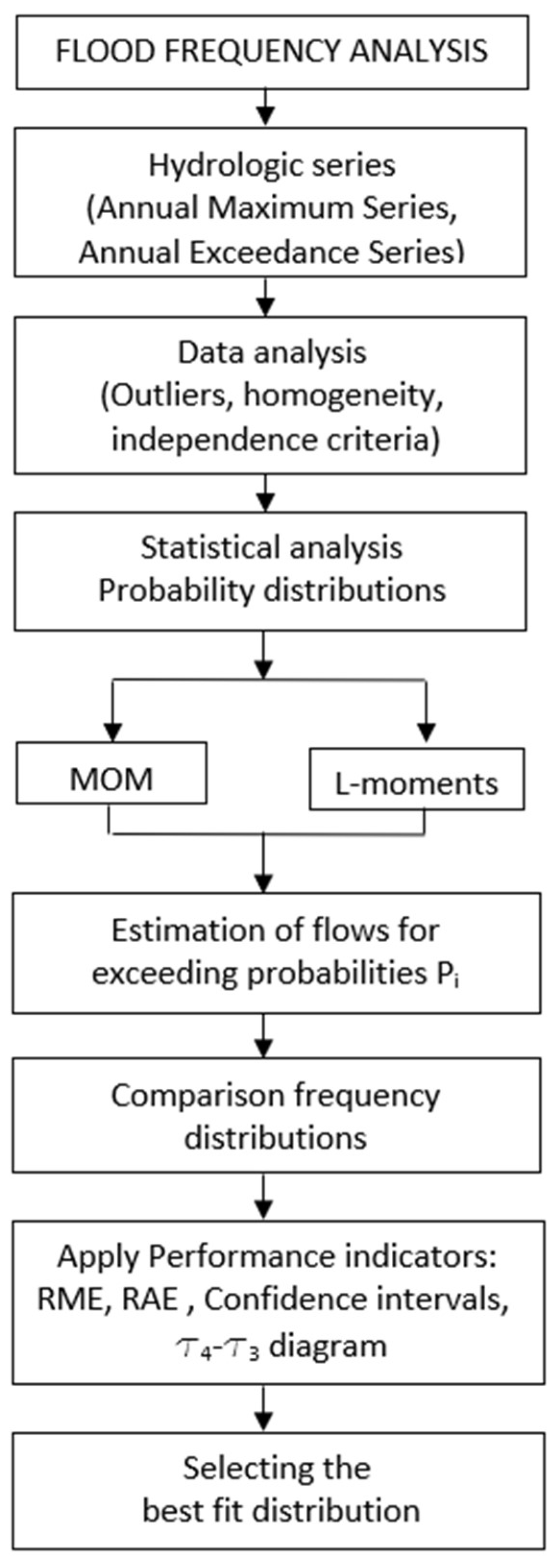
The determination of the maximum flows was carried out in stages according to Figure 1. The verification of the character of outliers (Grubbs, Pilon, Quartile method), homogeneity and independence of flows was carried out in the data curation phase. No outliers were detected.
The estimation of the parameters of the analyzed distributions was done with MOM and L-moments. The MOM estimation has the disadvantage that for high-order moments and small data series, in many cases, it generates unrealistic values because the high-order moments require correction [4,5,28,29]. For skewness, the correction can be made using the Bobee relation [26] or, as is the practice in Romania [22,30,31,32,33], being established according to the origin of the maximum flows by multiplying the coefficient of variation () by a coefficient reflecting this origin. In many cases, the choice is subjective and without rigor [22,34].
Considering that in many cases it is necessary to solve some systems of non-linear equations to estimate the parameters of the analyzed distributions, approximate relations for estimating the parameters were determined in the case of distributions where skewness and L-skewness depend on a single parameter. In addition, for a simplified and fast calculation that takes into account the fact that the inverse function can be expressed with the frequency factor for both MOM [4,23,34] and L-moments [23], the approximation relations of the factor of frequency (and the coefficients of these relations) are for the most frequent exceedance probabilities in the analysis of maximum flows. The estimation errors of both the parameters and the frequency factors are between 10−3 and 10−4.
The quantile results are compared with those of the Pearson III distribution, which is the “parent” distribution in Romania in the analysis of extreme events in hydrology, especially in the flood frequency analysis [22,30,31].
2.1. Probability Distributions
In Table 2 the probability density function, ; the complementary cumulative distribution function, , and the quantile function, , are presented for analyzed distributions [4,5,6,7,8,9,14,15,16,17]. All and of the analyzed distributions were determined using the methodology presented in the Supplementary file using only .
2.2. Parameter Estimation
The parameters estimation of the analyzed statistical distributions is presented for the MOM and the L-moments method, some of the most used methods in hydrology for parameter estimation [3,4,5,7,22].
2.2.1. Generalized Pareto Type IV (PGIV4)
The equations needed to estimate the parameters with MOM have the following expressions:
Because they are too long, the relations for estimating the skewness and the kurtosis are presented in Appendix F.
The equations needed to estimate the parameters with L-moments have the following expressions:
where represent the first four linear moments.
2.2.2. Generalized Pareto Type IV (PGIV3)
The distribution represents a particular case of the Pareto IV distribution when the position parameter . It is also known as the beta_p or Singh–Maddala distribution [9,35].
The equations needed to estimate the parameters with MOM have the following expressions:
2.2.3. Generalized Pareto Type III (PGIII)
The shape parameter can be obtained approximately depending on the skewness coefficient using the following function:
If :
The equations needed to estimate the parameters with L-moments have the following expressions:
2.2.4. Generalized Pareto Type II (PGII)
The shape parameter can be obtained approximately depending on the skewness coefficient using the following functions:
If :
If :
The frequency factor (for MOM), presented in Appendix B, can be obtained approximately using a polynomial function of skewness and probability, whose coefficients are presented in Table A4 from Appendix D.
The equations needed to estimate the parameters with L-moments have the following expressions:
Based on these equations, the parameters have the following expressions:
The frequency factor (for L-moments) can be obtained approximately using a polynomial function depending on skewness and probability, whose coefficients are presented in Table A5 from Appendix D.
2.2.5. Generalized Pareto Type I (PGI)
The equations needed to estimate the parameters with MOM have the following expressions:
The shape parameter can be obtained approximately depending on the skewness coefficient using the following functions:
If :
If :
The equations needed to estimate the parameters with MOM have the following expressions:
Based on these equations, the parameters have the following expressions:
2.2.6. The Five-Parameter Wakeby Distribution (WK5)
The equations needed to estimate the parameters with MOM have the following expressions:
The equations for skewness and kurtosis are presented in Appendix E.
3. Case Study
The presented case study consists in the determination of the maximum annual flows, on the Prigor River, Romania, using the proposed probability distributions.
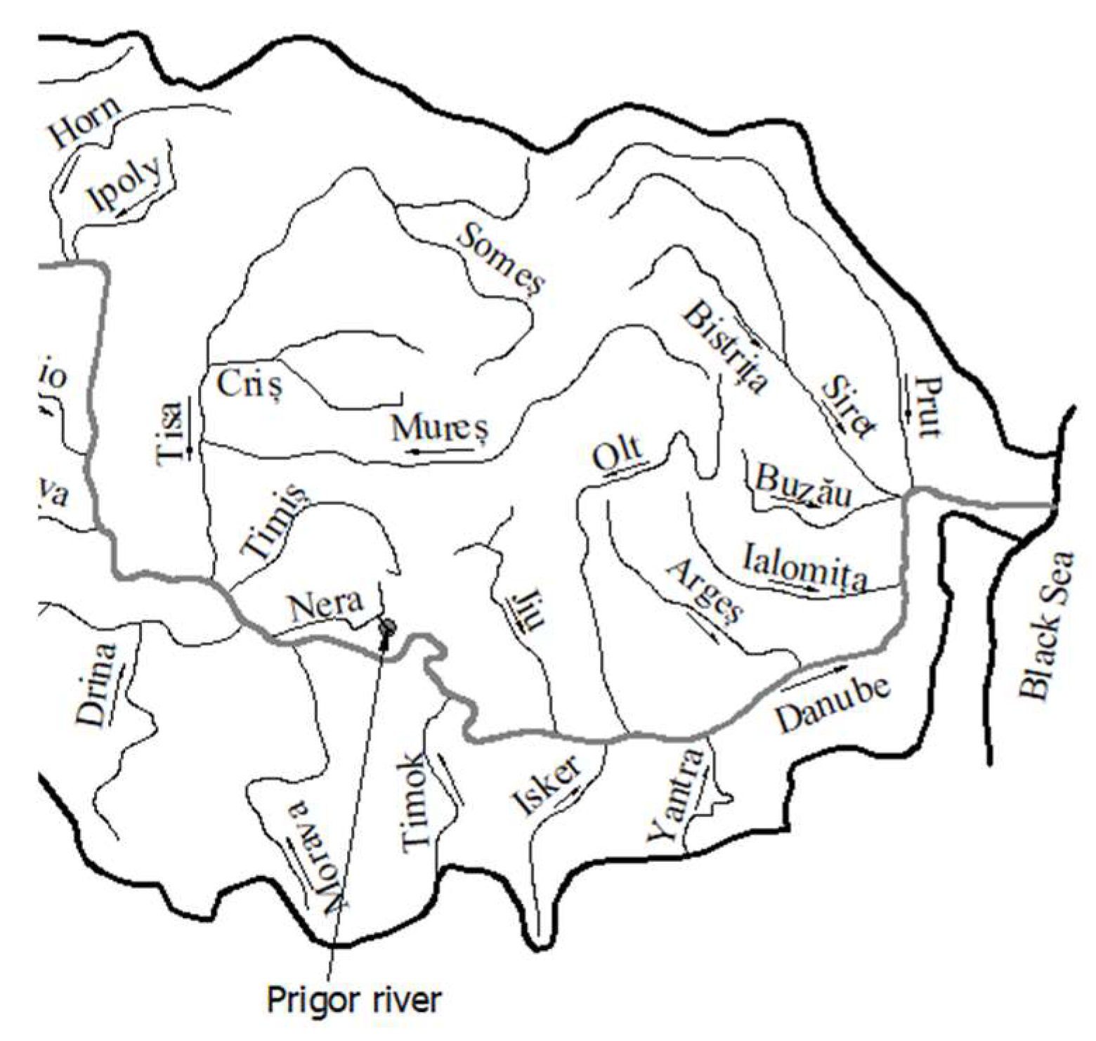
The Prigor River is the left tributary of the Nera River, and it is located in the south-western part of Romania, as shown in Figure 2. The geographical coordinates of the location are 44°55′25.5″ N 22°07′21.7″ E.
In the section of the hydrometric station, the watershed area is 141 km2 and the average altitude is 729 m. The river has a length of 33 km, with an average slope of 22‰ and a sinuosity coefficient of 1.83.
There are 31 annual maximum flows; the values are presented in Table 4.
For the analysis with the AES, the maximum flows resulting from the selection are presented in Table 5.
The main statistical indicators of the data series are presented in Table 6.
4. Results
The proposed distributions from the Generalized Pareto family, were applied to perform a flood frequency analysis using the annual maximum series (AMS) and the annual exceedance series (AES) analysis, on the Prigor River.
The MOM and the L-moments method were used to estimate the parameters of the distributions. For the MOM, the skewness coefficient was chosen depending on the origin of the flows according to Romanian regulations [22,30] based on some multiplication coefficients for the coefficient of variation (). For the Prigor River, the multiplication coefficient 3, applied to the coefficient of variation, resulted in a skewness of 2.29 for AMS and 1.786 for AES. In Table 7 and Table 8 the resulted values of quantile distributions for some of the most common exceedance probabilities in flood frequency analysis are presented.
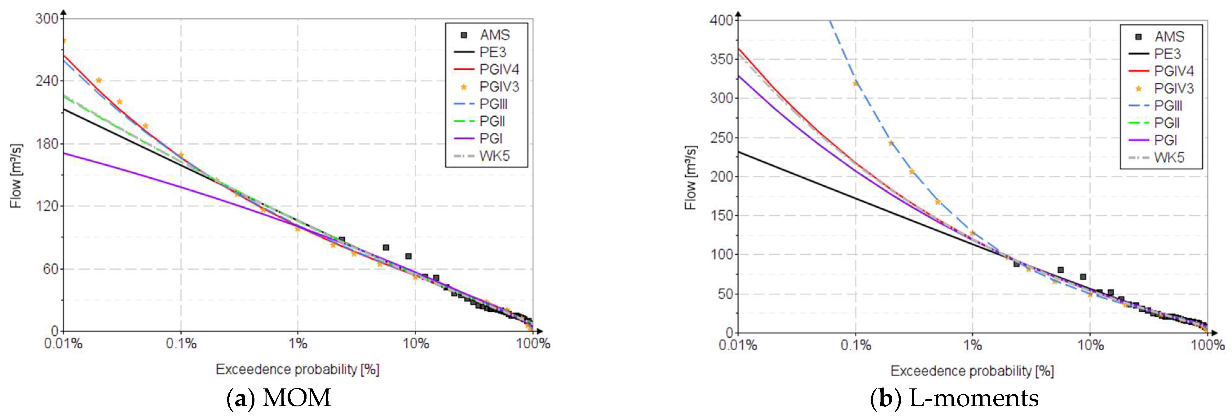
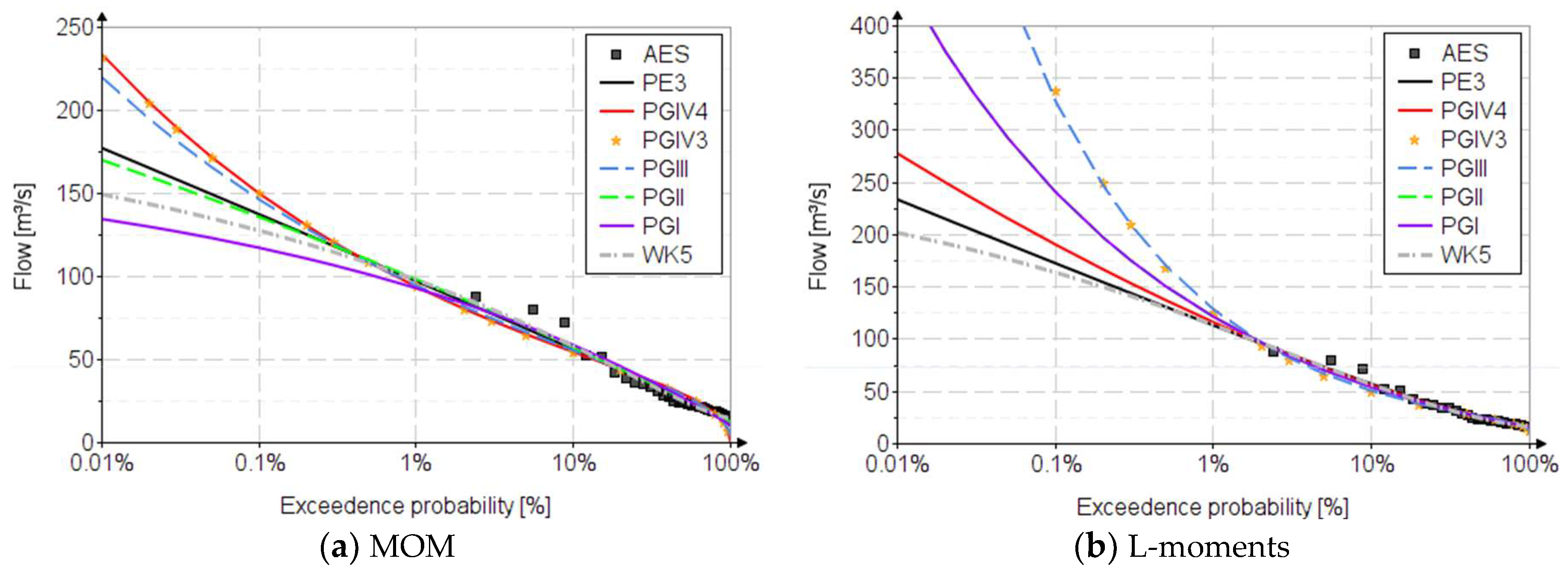
Figure 3 and Figure 4 show the fitting distributions for AMS and AES for the Prigor River. For plotting positions, the Alexeev formula was used [2].
In Figure S1, from the Supplementary Material, the confidence interval for each analyzed distribution is presented, both for the MOM and L-moments, using Chow’s relation [4,36] for a 95% confidence level.
Table 9 shows the values of the distributions parameters for the two methods of estimating and for both the AMS and AES.
Considering that it is desired to apply the distributions using the L-moments method, choosing the best distribution is based on the L-skewness () and L-kurtosis () values and diagram. The values of the RME and RAE indicators [38,39,40] are presented informatively, knowing that they are relevant only in the area of the observed data.
5. Discussions
In this article, the applicability of the distributions from the Generalized Pareto family in flood frequency analysis was analyzed using the Prigor River as a case study.
The analysis was performed using the AMS and AES. As can be seen both graphically (Figure 4) and tabularly (Table 7), the analysis with the AMS is more conservative than the analysis with the AES.
The main advantage of the AMS analysis is the ease of data selection, these being chosen as the maximum flow corresponding to each year. The disadvantage of the analysis is the use of maximum flows characteristic of each year, which do not always represent floods. These values located in the right-hand (high probabilities) lead to a steeper graph with higher values of quantiles in the field of low probabilities (left-hand).
The advantage of the analysis with AES is that the flows of the data series always represent floods. The disadvantage is the greater effort in data selection, through additional analyzes regarding data independence, respecting the condition that these maximum flows do not come from the same flood.
The estimation methods of the analyzed distribution parameters were performed for the MOM (standard method in Romania) and L-moments, two of the most used estimation methods in hydrology.
For the MOM analysis, the skewness was chosen depending on the origin of the flows, as is the hydrological practice in Romania. The use of multiplication coefficients for the calculation of the corrected skewness is an outdated method based on principles from the abrogated norms and a legacy from the USSR normative standards.
All analyzed distributions represent particular cases of the Generalized Pareto distribution, which are distributions of three and four parameters. The Wakeby distribution, which is a five-parameter distribution, was analyzed because it has as its particular case the PGII distribution, which is a quantile function whose structure is made up of two quantile functions of the PGII distribution.
All the results obtained in the case study are presented in comparison to the Pearson III distribution, which is considered the “parent” distribution in Romania, for the most used exceedance probabilities in hydrology.
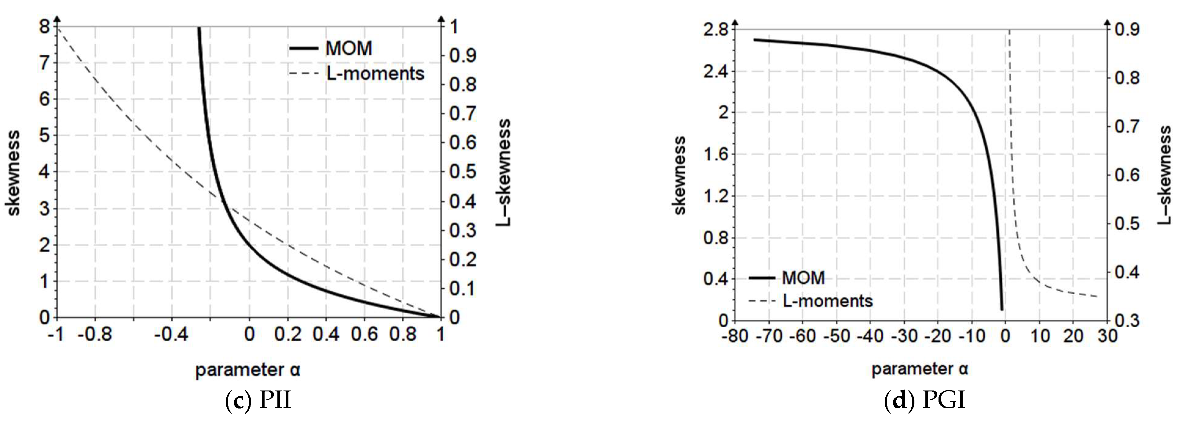
Considering that it is desired to implement the L-moments method in Romania, according to Tabel 10 and Tabel 11, the best-fitted distributions are the PGIV4 and WK5 distributions, which best approximate the statistical indicators of the data set, and . The PGII and PGI distributions give satisfactory results because the natural values and of the distributions are close to those of the data sets.
For the PE3, PGIV3, PGIII, PGII and PGI, which are three parameter distributions, the resulting values are characterized by a high degree of uncertainty, especially in the area of small exceedance probabilities (left-hand), due to the fact that a proper calibration of the higher moments cannot be done. The confidence intervals for the analyzed distributions are presented in the Supplementary Material.
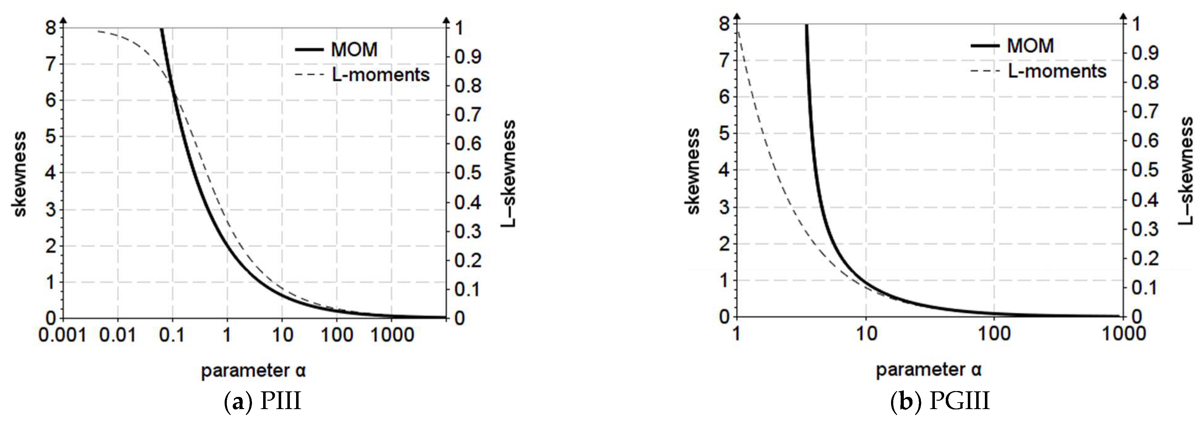
As observed in other materials [24], the apparent stability of the Pearson III distribution is due to the fact that the variation of the shape parameter for the two estimation methods does not differ much, except in the upper area of and . The same cannot be said, for example, about the PGI, PGII and PGIII distributions, in which the variation is extremely large. Figure 5 shows the variation graph of the shape parameter for the PE3, PGIII, PGII and PGI distributions. As it could be observed in Section 2.1, both skewness and L-skewness depend only on the shape coefficient .
The results of the quantiles obtained with the L-moments method, for the PGII and PGI distributions, both for the AES and AMS, presented in Table 4 and Table 5, are the same, the two distributions being mutual special cases. The WK5 and PGIV4 distributions best approximate, as expected, the values of the indicators obtained with L-moments, which are distributions of five and four parameters, respectively.
Figure 6 shows the variation diagram of the distributions as well as their relation to the values of the two indicators of the data sets.
Regarding the results obtained with MOM, for AES it can also be observed that the PGII and WK5 distributions have extremely close quantile values, which is due to the fact that for the same they correspond to the same value of , the WK5 distribution becoming the PGII distribution, as it was highlighted in other materials [4,8,9,22]. This is due to the choice of skewness based on the origin of the maximum flows. This is another disadvantage of using MOM in Romania.
Concerning the WK5 distribution, although it is a distribution that was introduced in flood frequency analysis to achieve the so-called “separation effect” described by Matalas [9,22], it can be seen that it is extremely sensitive depending on the analysis used (AMS or AES), and this is due to the particular cases in which it can take.
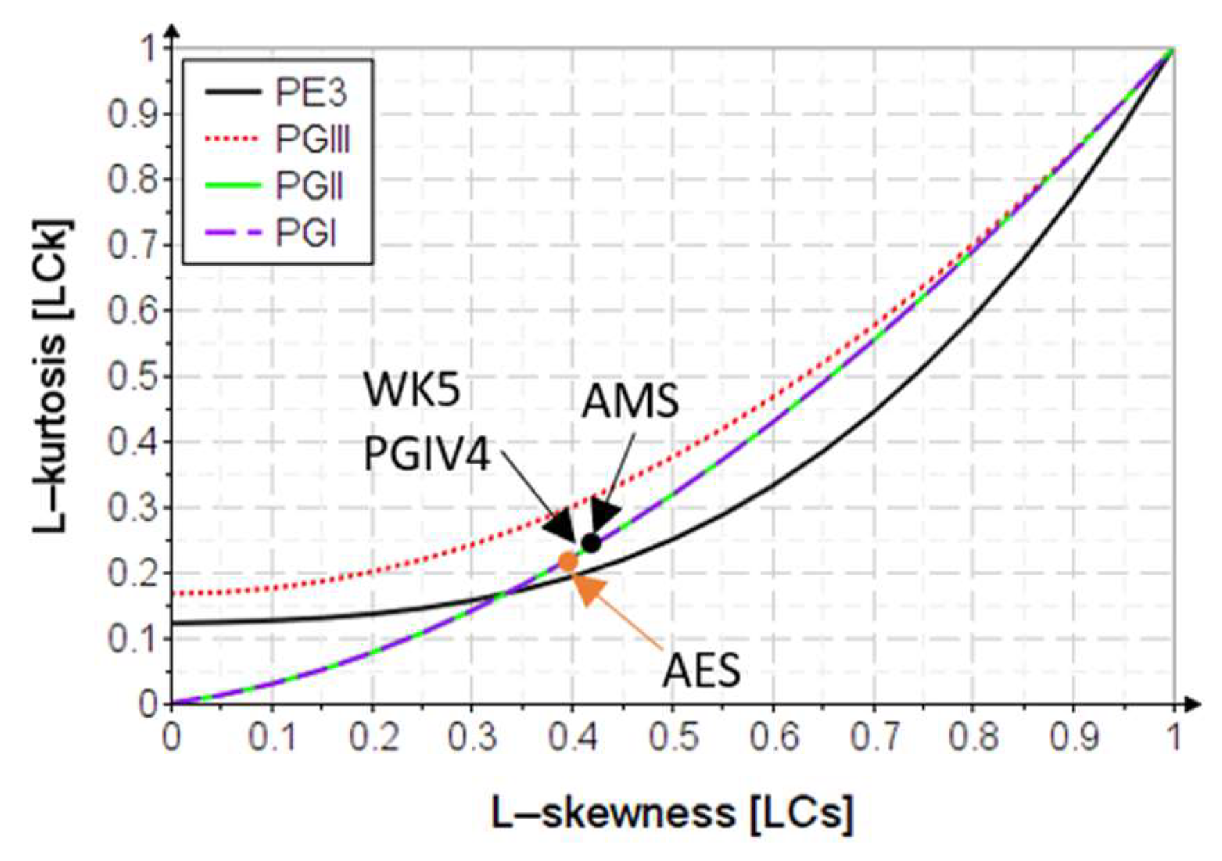
Figure 7 shows the skewness ()-kurtozis () variation diagram of the distributions.
6. Conclusions
The Generalized Pareto distribution represents a usual distribution used in the analysis of extreme events in hydrology. In flood frequency analysis this is especially applied using the partial series of maximum flows.
This article presents five distributions of three, four and five parameters that represent different forms of the Generalized Pareto distribution, some of them received limited attention in flood frequency analysis.
These distributions were analyzed (besides other families of distributions) in the research carried out in the Faculty of Hydrotechnics regarding the elaboration of a norm in Romania for the frequency analysis using the L-moments method.
The main purpose of the article was to identify other distributions from the same family that have applicability in flood frequency analysis using both AMS and AES.
For the transparency and ease of use of these distributions, all the necessary elements for their use are presented, such as the exact and approximate relations of the parameters’ estimation, and of the frequency factors, which eliminates the need for iterative numerical calculation, thus facilitating their applicability.
The performances of these distributions were verified in flood frequency analysis of the Prigor River, using the Annual Maximum Series and the Annual Exceedance Series.
The results were evaluated using the values of and , based on the diagram, compared to that of the data sets, which is the easiest and most accessible selection criterion.
Based on this study’s results, and also from the research carried out in the Faculty of Hydrotechnics for other sites, for flood frequency analysis and the L-moments estimation method, good candidates, from the Generalized Pareto family, are the PGIV4 and WK5 distributions, which are distributions of four and five parameters, which have the advantage that they can calibrate all linear moments.
Regarding the Wakeby distribution, this requires an additional analysis because in some cases it turns into the PGII distribution, which is a three-parameter distribution that does not achieve a satisfactory calibration of the linear moments.
In general, the three parameters distributions can be used in the analysis with L-moments, but the selection of their use must be made based on the - diagram so that the natural values and of the distribution to be very close to those of the observed data. Based on the work of Anghel si Ilinca [23], in Appendix A the diagram for a wide range of distributions used in hydrology is presented.
Mathematical support in statistical analysis is useful because the use of software (EasyFit, HEC-SSP, etc) without knowledge of mathematical foundations often leads to superficial analyzes with negative consequences. Another important aspect of the presentation of all the mathematical elements necessary for the application of these distributions is the fact that the software dedicated to statistical analysis is limited and does not offer the possibility of choosing the skewness coefficient depending on the origin of the maximum flows, as is the practice in Romania.
The research in this article is part of a more complex research carried out within the Faculty of Hydrotechnics, with the main aim of establishing the necessary guidelines for a robust, clear and concise norm regarding the determination of the maximum flow using the L-moment estimation method.
Supplementary Materials
The following supporting information can be downloaded at: https://www.mdpi.com/article/10.3390/w15081557/s1, Figure S1: The probability distributions curves with Confidence Intervals.
Author Contributions
Conceptualization, C.I. and C.G.A.; methodology, C.I. and C.G.A.; software, C.I. and C.G.A.; validation, C.I. and C.G.A.; formal analysis, C.I. and C.G.A.; investigation, C.I. and C.G.A.; resources, C.I. and C.G.A.; data curation, C.I. and C.G.A.; writing—original draft preparation, C.I. and C.G.A.; writing—review and editing, C.I. and C.G.A.; visualization, C.I. and C.G.A.; supervision, C.I. and C.G.A.; project administration, C.I. and C.G.A.; funding acquisition, C.I. and C.G.A. All authors have read and agreed to the published version of the manuscript.
Funding
This research received no external funding.
Data Availability Statement
Not applicable.
Conflicts of Interest
The authors declare no conflict of interest.
Abbreviations
| MOM | the method of ordinary moments |
| L-moments | the method of linear moments |
| expected value; arithmetic mean | |
| standard deviation | |
| coefficient of variation | |
| coefficient of skewness; skewness | |
| coefficient of kurtosis; kurtosis | |
| linear moments | |
| coefficient of variation based on the L-moments method | |
| coefficient of skewness based on the L-moments method | |
| coefficient of kurtosis based on the L-moments method | |
| Distr. | Distributions |
| RME | relative mean error |
| RAE | relative absolute error |
| xi | observed values |
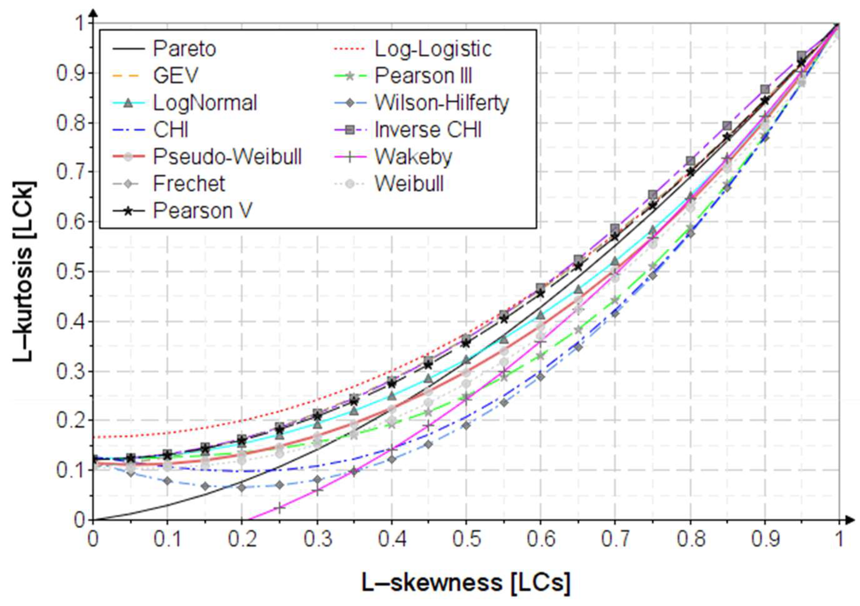
Appendix A. The Variation of the L-Kurtosis—L-Skewness
In the next section the variation of the L-kurtosis depending on the positive L-skewness, obtained with the L-moments method, for certain theoretical distributions often used in hydrology is presented.
Figure A1.
The variation diagram of .

Appendix B. The Frequency Factors for the Analyzed Distributions
Table A1 shows the expressions of the frequency factors for MOM and L-moments.

Table A1.
Frequency factors.
| Distribution | ||
|---|---|---|
| Quantile Function (Inverse Function) | ||
| Method of Ordinary Moments (MOM) | L-Moments | |
| PGIV4 | ||
| PGIV3 | ||
| PGIII | ||
| PGII | ||
| PGI | ||
| WK5 | ||
Appendix C. Estimation of the Frequency Factor for the PGIII Distribution
The frequency factor, for MOM, can be estimated using the following polynomial function:
Table A2.
The frequency factor for estimation with MOM.
| P [%] | a | b | c | d | e | f | g | h |
|---|---|---|---|---|---|---|---|---|
| 0.01 | 5.111737 | 2.313409 | 1.34999 | −0.776028 | 0.182704 | −0.0232091 | 1.5563 × 10⁻³ | −4.330 × 10⁻⁵ |
| 0.1 | 3.808941 | 1.377403 | 345331 | −0.318752 | 0.0903167 | −0.0130843 | 9.7470 × 10⁻⁴ | −2.960 × 10⁻⁵ |
| 0.5 | 2.912620 | 0.812083 | 0.0170251 | −0.114635 | 0.0394326 | −6.29710 × 10⁻³ | 4.9970 × 10⁻⁴ | −1.590 × 10⁻⁵ |
| 1 | 2.527259 | 0.600436 | −0.0535487 | −0.0565675 | 0.0233015 | 3.98010 × 10⁻³ | 3.2800 × 10⁻⁴ | 1.070 × 10⁻⁵ |
| 2 | 2.140031 | 0.411098 | −0.0911407 | −0.0147256 | 0.0107835 | −2.10400 × 10⁻³ | 1.8480 × 10⁻⁴ | −6.200 × 10⁻⁶ |
| 3 | 1.911447 | 0.311395 | −0.100372 | 2.88960 × 10⁻³ | 5.08580 × 10⁻³ | −1.21600 × 10⁻³ | 1.1520 × 10⁻⁴ | −4.100 × 10⁻⁶ |
| 5 | 1.619324 | 0.197967 | −0.100797 | 0.0185338 | −4.64200 × 10⁻⁴ | −3.15600 × 10⁻⁴ | 4.3000 × 10⁻⁵ | −1.700 × 10⁻⁶ |
| 10 | 1.208950 | 0.066749 | −0.0847851 | 0.0291844 | −5.24780 × 10⁻³ | 5.25900 × 10⁻⁴ | −2.7400 × 10⁻⁵ | 6.000 × 10⁻⁷ |
| 20 | 0.763538 | −0.0362722 | −0.0531111 | 0.0286703 | −6.99220 × 10⁻³ | 9.32800 × 10⁻⁴ | −6.5700 × 10⁻⁵ | 1.900 × 10⁻⁶ |
| 40 | 0.224364 | −0.103222 | −6.80020 × 10⁻³ | 0.0162353 | −5.34190 × 10⁻³ | 8.40400 × 10⁻⁴ | −6.63000 × 10⁻⁵ | 2.100 × 10⁻⁶ |
| 50 | 0.001255 | −0.111838 | 0.0119116 | 8.67100 × 10⁻³ | −3.76100 × 10⁻³ | 6.53200 × 10⁻⁴ | −5.44000 × 10⁻⁵ | 1.8000 × 10⁻⁶ |
| 80 | −0.762791 | −0.0547579 | 0.0593627 | −0.0207334 | 3.89270 × 10⁻³ | −4.16000 × 10⁻⁴ | 2.37000 × 10⁻⁵ | −6.000 × 10⁻⁷ |
| 90 | −1.210684 | 0.0415455 | 0.0668030 | −0.036012 | 8.85020 × 10⁻³ | −1.19170 × 10⁻³ | 8.48000 × 10⁻⁵ | −2.500 × 10⁻⁶ |
The frequency factor, for L-moments, can be estimated using the following rational function:
Table A3.
The frequency factor for estimation with L-moments.
| P [%] | a | b | c | d | e | f | g | h |
|---|---|---|---|---|---|---|---|---|
| 0.01 | 9.0865 | −9.0870 | −5.6824 | 14.136 | −19.532 | 15.682 | −6.8872 | 1.2851 |
| 0.1 | 6.8300 | −6.8367 | −4.3709 | 8.5137 | −9.3692 | 6.1000 | −2.2178 | 0.35120 |
| 0.5 | 5.3161 | −5.3440 | −3.2817 | 4.4099 | −2.2009 | −1.0766 | 1.7928 | 0.61653 |
| 1 | 4.6040 | −4.6529 | −2.9168 | 3.6177 | −1.7699 | −0.69899 | 1.2546 | −0.43830 |
| 2 | 3.8961 | −3.9826 | −2.5218 | 2.8156 | −1.2339 | −0.62320 | 0.99972 | −0.35026 |
| 3 | 3.4784 | −3.5994 | −2.2840 | 2.4127 | −1.0762 | −0.39996 | 0.73125 | −0.26304 |
| 5 | 2.9457 | −3.1313 | −1.9655 | 1.9096 | −0.81060 | −0.29906 | 0.55319 | −0.20219 |
| 10 | 2.1976 | −2.5343 | −1.4975 | 1.3114 | −0.53308 | −0.15403 | 0.33379 | −0.12411 |
| 20 | 1.3864 | −2.0186 | −0.95952 | 0.81735 | −0.27803 | −0.074878 | 0.18663 | −0.059390 |
| 40 | 0.40582 | −0.40582 | −0.25879 | 0.38534 | 0.16327 | −0.042751 | −0.062078 | 0.088377 |
| 50 | 1.934 × 10⁻⁴ | −1.6511 | 0.033144 | 0.37384 | 0.19857 | 0.011770 | −0.031091 | 0.064863 |
| 80 | −1.3869 | −0.52845 | −0.095705 | 1.2009 | −0.42838 | 0.047547 | 0.40683 | −0.21635 |
| 90 | −2.1977 | 1.0582 | −0.12265 | 0.70118 | −0.41310 | −0.11862 | 0.17678 | −0.084297 |
Appendix D. Estimation of the Frequency Factor for the PGII Distribution
The frequency factor, for MOM, can be estimated using the following polynomial function:
Table A4.
The frequency factor for estimation with MOM.
| P [%] | a | b | c | d | e | f | g | h |
|---|---|---|---|---|---|---|---|---|
| 0.01 | 1.932014 | 0.061904 | 2.87112 | −0.795586 | 0.0495418 | 1.03747 × 10⁻² | −1.7871 × 10⁻³ | 7.910 × 10⁻⁵ |
| 0.1 | 1.809609 | 0.670411 | 2.12699 | −1.15732 | 0.284537 | −3.77979 × 10⁻² | 2.6299 × 10⁻³ | −7.530 × 10⁻⁵ |
| 0.5 | 1.704417 | 1.213220 | 0.762347 | −0.651934 | 0.198072 | −3.05909 × 10⁻² | 2.3988 × 10⁻³ | −7.580 × 10⁻⁵ |
| 1 | 1.664419 | 1.314780 | 0.178438 | −0.355564 | 0.125632 | −2.09008 × 10⁻² | 1.7176 × 10⁻³ | −5.610 × 10⁻⁵ |
| 2 | 1.622183 | 1.265729 | −0.290832 | −0.0764258 | 0.0500117 | −9.92700 × 10⁻³ | 8.9160 × 10⁻⁴ | −3.080 × 10⁻⁵ |
| 3 | 1.590286 | 1.151049 | −0.479305 | 0.0583412 | 0.0103575 | −3.85500 × 10⁻³ | 4.1630 × 10⁻⁴ | −1.570 × 10⁻⁵ |
| 5 | 1.530888 | 0.909001 | −0.598849 | 0.179061 | −0.0288591 | 2.47620 × 10⁻³ | −9.6700 × 10⁻⁵ | 9.000 × 10⁻⁷ |
| 10 | 1.377562 | 0.424384 | −0.522494 | 0.228357 | −0.0536328 | 7.14020 × 10⁻³ | −5.0690 × 10⁻⁴ | 1.490 × 10⁻⁵ |
| 20 | 1.047703 | −0.1346753 | −0.197916 | 0.136073 | −0.0393659 | 5.98720 × 10⁻³ | −4.6780 × 10⁻⁴ | 1.480 × 10⁻⁵ |
| 40 | 0.355375 | −0.4660863 | 0.182363 | −0.0347085 | 2.20900 × 10⁻³ | 2.60000 × 10⁻⁴ | −4.8700 × 10⁻⁵ | 2.100 × 10⁻⁶ |
| 50 | 0.0051002 | −0.428129 | 0.242055 | −0.0758534 | 0.0142094 | −1.57970 × 10⁻³ | 9.61000 × 10⁻⁵ | −2.5000 × 10⁻⁶ |
| 80 | −1.042946 | 0.1095022 | 0.0744175 | −0.0546187 | 0.0156946 | −2.36020 × 10⁻³ | 1.82600 × 10⁻⁴ | −5.700 × 10⁻⁶ |
| 90 | −1.389758 | 0.3823067 | −0.0662687 | −9.67300 × 10⁻³ | 6.70430 × 10⁻³ | −1.27020 × 10⁻³ | 1.09700 × 10⁻⁴ | −3.700 × 10⁻⁶ |
The frequency factor, for L-moments, can be estimated using the following polynomial function:
Table A5.
The frequency factor for estimation with L-moments.
| P [%] | a | b | c | d | e | f | g | h | i | j |
|---|---|---|---|---|---|---|---|---|---|---|
| 0.01 | 2.8976 | 16.049 | −166.33 | 2107.2 | −11711 | 41260 | −84364 | 1.0671 × 10⁵ | −68465 | 14604 |
| 0.1 | 2.9921 | 7.9122 | 21.160 | 46.340 | 207.03 | −394.80 | 1467.1 | −2026.5 | 667.72 | − |
| 0.5 | 2.9751 | 7.0733 | 21.320 | 5.3452 | 97.924 | −99.393 | −95.564 | −59.326 | − | − |
| 1 | 2.9389 | 6.8741 | 14.223 | 10.895 | 33.199 | −116.24 | 47.113 | − | − | − |
| 2 | 2.8667 | 6.5598 | 3.8790 | 28.740 | −66.614 | 23.564 | − | − | − | − |
| 3 | 2.8214 | 5.3368 | 6.0252 | 1.9543 | −31.305 | 14.174 | − | − | − | − |
| 5 | 2.7060 | 3.9951 | 4.1471 | −13.220 | −2.6956 | 4.0738 | − | − | − | − |
| 10 | 2.4017 | 2.0082 | −1.6983 | −9.9252 | 7.8868 | −1.6725 | − | − | − | − |
| 20 | 1.7989 | −0.48676 | −4.2616 | 1.0072 | 1.7490 | −0.80770 | − | − | − | − |
| 40 | 0.60025 | −2.4049 | −0.31267 | 2.3727 | −1.6966 | 0.44147 | − | − | − | − |
| 50 | 3.8891 × 10⁻⁴ | −2.3323 | 1.3905 | 0.48092 | −0.81390 | 0.27475 | − | − | − | − |
| 80 | −1.8003 | 0.52569 | 1.0120 | −1.3741 | 0.86642 | −0.22985 | − | − | − | − |
| 90 | −2.4001 | 2.1286 | −0.96924 | 0.23252 | 0.041754 | −0.033573 | − | − | − | − |
Appendix E. The Skewness and Kurtosis for the WK5 Distribution
Appendix F. The Skewness and Kurtosis for the PGIV Distribution
References
- Popovici, A. Dams for Water Accumulations; Technical Publishing House: Bucharest, Romania, 2002; Volume 2. [Google Scholar]
- Teodorescu, I.; Filotti, A.; Chiriac, V.; Ceausescu, V.; Florescu, A. Water Management; Ceres Publishing House: Bucharest, Romania, 1973. [Google Scholar]
- Hosking, J.R.M.; Wallis, J.R. Regional Frequency Analysis: An Approach Based on L-moments; Cambridge University Press: Cambridge, UK, 1997. [Google Scholar] [CrossRef]
- Rao, A.R.; Hamed, K.H. Flood Frequency Analysis; CRC Press LLC: Boca Raton, FL, USA, 2000. [Google Scholar]
- Singh, V.P. Entropy-Based Parameter Estimation in Hydrology; Springer Science + Business Media: Dordrecht, The Netherlands, 1998; ISBN 978-90-481-5089-2/978-94-017-1431-0. [Google Scholar] [CrossRef]
- Gubareva, T.S.; Gartsman, B.I. Estimating Distribution Parameters of Extreme Hydrometeorological Characteristics by L-Moment Method. Water Resour. 2010, 37, 437–445. [Google Scholar] [CrossRef]
- Greenwood, J.A.; Landwehr, J.M.; Matalas, N.C.; Wallis, J.R. Probability Weighted Moments: Definition and Relation to Parameters of Several Distributions Expressable in Inverse Form. Water Resour. Res. 1979, 15, 1049–1054. [Google Scholar] [CrossRef]
- Houghton, J.C. Birth of a parent: The Wakeby distribution for modeling flood flows. Water Resour. Res. 1978, 14, 1105–1109. [Google Scholar] [CrossRef]
- Crooks, G.E. Field Guide to Continuous Probability Distributions; Berkeley Institute for Theoretical Science: Berkeley, CA, USA, 2019. [Google Scholar]
- Yang, T.; Shao, Q.X.; Hao, Z.C.; Chen, X.; Zhang, Z.X.; Xu, C.Y.; Sun, L.M. Regional frequency analysis and spatio-temporal pattern characterization of rainfall extremes in the Pearl River Basin, China. J. Hydrol. 2010, 380, 386–405. [Google Scholar] [CrossRef]
- Zakaria, Z.A.; Shabri, A. Regional frequency analysis of extreme rainfalls using partial L-moments method. Theor. Appl. Climatol. 2013, 113, 83–94. [Google Scholar] [CrossRef]
- Zhou, C.R.; Chen, Y.F.; Huang, Q.; Gu, S.H. Higher moments method for generalized Pareto distribution in flood frequency analysis. IOP Conf. Ser. Earth Environ. Sci. 2017, 82, 012031. [Google Scholar] [CrossRef]
- Martins, A.L.A.; Liska, G.R.; Beijo, L.A.; Menezes, F.S.D.; Cirillo, M.Â. Generalized Pareto distribution applied to the analysis of maximum rainfall events in Uruguaiana, RS, Brazil. SN Appl. Sci. 2020, 2, 1479. [Google Scholar] [CrossRef]
- Ciupak, M.; Ozga-Zielinski, B.; Tokarczyk, T.; Adamowski, J. A Probabilistic Model for Maximum Rainfall Frequency Analysis. Water 2021, 13, 2688. [Google Scholar] [CrossRef]
- Shao, Y.; Zhao, J.; Xu, J.; Fu, A.; Wu, J. Revision of Frequency Estimates of Extreme Precipitation Based on the Annual Maximum Series in the Jiangsu Province in China. Water 2021, 13, 1832. [Google Scholar] [CrossRef]
- Ashkar, F.; Ouarda, T.B. On some methods of fitting the generalized Pareto distribution. J. Hydrol. 1996, 177, 117–141. [Google Scholar] [CrossRef]
- Mohsen, S.; Zulkifli, Y.; Fadhilah, Y. Comparison of Distribution Models for Peak flow, Flood Volume and Flood Duration. Res. J. Appl. Sci. Eng. Technol. 2013, 6, 733–738. [Google Scholar]
- Swetapadma, S.; Ojha, C.S.P. Technical Note: Flood frequency study using partial duration series coupled with entropy principle. Hydrol. Earth Syst. Sci. Discuss. 2021. preprint. [Google Scholar] [CrossRef]
- Rahman, A.S.; Rahman, A.; Zaman, M.A.; Haddad, K.; Ahsan, A.; Imteaz, M. A study on selection of probability distributions for at-site flood frequency analysis in Australia. Nat. Hazards 2013, 69, 1803–1813. [Google Scholar] [CrossRef]
- Drissia, T.K.; Jothiprakash, V.; Anitha, A.B. Flood Frequency Analysis Using L Moments: A Comparison between At-Site and Regional Approach. Water Resour. Manag. 2019, 33, 1013–1037. [Google Scholar] [CrossRef]
- Hosking, J.R.M.; Wallis, J.R. Parameter and Quantile Estimation for the Generalized Pareto Distribution. Technometrics 1987, 29, 339–349. [Google Scholar] [CrossRef]
- Ilinca, C.; Anghel, C.G. Flood-Frequency Analysis for Dams in Romania. Water 2022, 14, 2884. [Google Scholar] [CrossRef]
- Anghel, C.G.; Ilinca, C. Hydrological Drought Frequency Analysis in Water Management Using Univariate Distributions. Appl. Sci. 2023, 13, 3055. [Google Scholar] [CrossRef]
- Anghel, C.G.; Ilinca, C. Parameter Estimation for Some Probability Distributions Used in Hydrology. Appl. Sci. 2022, 12, 12588. [Google Scholar] [CrossRef]
- Viglione, A.; Merz, R.; Salinas, J.L.; Blöschl, G. Flood frequency hydrology: 3. A Bayesian analysis. Water Resour. Res. 2013, 49, 675–692. [Google Scholar] [CrossRef]
- Gaume, E. Flood frequency analysis: The Bayesian choice. WIREs Water. 2018, 5, e1290. [Google Scholar] [CrossRef]
- Lang, M.; Ouarda, T.B.; Bobée, B. Towards operational guidelines for over-threshold modeling. J. Hydrol. 1999, 225, 103–117. [Google Scholar] [CrossRef]
- Bulletin 17B Guidelines for Determining Flood Flow Frequency; U.S. Department of the Interior, U.S. Geological Survey: Reston, VA, USA, 1981.
- Bulletin 17C Guidelines for Determining Flood Flow Frequency; U.S. Department of the Interior, U.S. Geological Survey: Reston, VA, USA, 2017.
- STAS 4068/1-82; Maximum Water Discharges and Volumes, Determination of Maximum Water Discharges and Volumes of Watercourses. The Romanian Standardization Institute: Bucharest, Romania, 1982.
- Diacon, C.P. Serban Hydrological Syntheses and Regionalizations; Technical Publishing House: Bucharest, Romania, 1994. [Google Scholar]
- Mandru, R.; Ioanitoaia, H. Ameliorative Hydrology; Agro-Silvica Publishing House: Bucharest, Romania, 1962. [Google Scholar]
- Constantinescu, M.; Golstein, M.; Haram, V.; Solomon, S. Hydrology; Technical Publishing House: Bucharest, Romania, 1956. [Google Scholar]
- Ministry of Regional Development and Tourism. The Regulations Regarding the Establishment of Maximum Flows and Volumes for the Calculation of Hydrotechnical Retention Constructions; Indicative NP 129-2011; Ministry of Regional Development and Tourism: Bucharest, Romania, 2012.
- Murshed, M.S.; Park, B.J.; Jeong, B.Y.; Park, J.S. LH-Moments of Some Distributions Useful in Hydrology. In Communications for Statistical Applications and Methods; The Korean Statistical Society: Seoul, Republic of Korea, 2009. [Google Scholar] [CrossRef]
- Chow, V.T.; Maidment, D.R.; Mays, L.W. Applied Hydrology; McGraw-Hill, Inc.: New York, NY, USA, 1988; ISBN 007-010810-2. [Google Scholar]
- Ministry of the Environment. The Romanian Water Classification Atlas, Part I—Morpho-Hydrographic Data on the Surface Hydrographic Network; Ministry of the Environment: Bucharest, Romania, 1992.
- Singh, K.; Singh, V.P. Parameter Estimation for Log-Pearson Type III Distribution by Pome. J. Hydraul. Eng. 1988, 1, 112–122. [Google Scholar] [CrossRef]
- Shaikh, M.P.; Yadav, S.M.; Manekar, V.L. Assessment of the empirical methods for the development of the synthetic unit hydrograph: A case study of a semi-arid river basin. Water Pract. Technol. 2021, 17, 139–156. [Google Scholar] [CrossRef]
- Gu, J.; Liu, S.; Zhou, Z.; Chalov, S.R.; Zhuang, Q. A Stacking Ensemble Learning Model for Monthly Rainfall Prediction in the Taihu Basin, China. Water 2022, 14, 492. [Google Scholar] [CrossRef]
Figure 1.
Methodological approach.

Figure 2.
The location of Prigor River and Prigor hydrometric station.

Figure 3.
The fitting distributions for AMS.

Figure 4.
The fitting distributions for AES.

Figure 5.
The variation of parameter .


Figure 6.
The diagram for analyzed distributions.

Figure 7.
The diagram for the analyzed distributions.

Table 1.
Novelty elements.
| New Elements | Distribution |
|---|---|
| Exact parameter estimation | PGIV4, PGI |
| Approximate estimation of parameters | PGIII, PGII, PGI |
| The frequency factor for MOM | PGIV4, PGIV3, PGIII, PGII, PGI, WK5 |
| The frequency factor for L-moments | PGIV4, PGIV3, PGIII, PGII, PGI, WK5 |
| Approximate estimation of the frequency factor | PGIII, PGII |
| Raw and central moments * | PGIV, PGIII, PGII |
* are presented in the Supplementary File.
Table 2.
The analyzed probability distributions.
| Distr. | |||
|---|---|---|---|
| PGIV4 | |||
| PGIV3 | |||
| PGIII | |||
| PGII | |||
| PGI | |||
| WK5 | No closed form | No closed form |
Table 3.
The morphometric characteristics.
| Length [km] | Average Stream Slope [‰] | Sinuosity Coefficient [-] | Average Altitude [m] | Watershed Area [km2] |
|---|---|---|---|---|
| 33 | 22 | 1.83 | 713 | 153 |
Table 4.
The AMS from the Prigor hydrometric station.
| AMS | ||||||||||||
| 1990 | 1991 | 1992 | 1993 | 1994 | 1995 | 1996 | 1997 | 1998 | 1999 | 2000 | ||
| Flow | [m3/s] | 9.96 | 15 | 10.1 | 14.8 | 7.30 | 21.2 | 18.2 | 21.4 | 13.1 | 14.5 | 35 |
| 2001 | 2002 | 2003 | 2004 | 2005 | 2006 | 2007 | 2008 | 2009 | 2010 | 2011 | ||
| Flow | [m3/s] | 19.9 | 22.1 | 11.8 | 80.3 | 88 | 51.6 | 72.2 | 16.2 | 42.6 | 28.5 | 12.8 |
| 2012 | 2013 | 2014 | 2015 | 2016 | 2017 | 2018 | 2019 | 2020 | ||||
| Flow | [m3/s] | 31.2 | 24.1 | 52.2 | 21.1 | 18.9 | 6.40 | 24.9 | 15.1 | 36.6 | ||
Table 5.
The AES from the Prigor hydrometric station.
| AES | ||||||||||||
| 1995 | 1996 | 1997 | 2000 | 2001 | 2002 | 2004 | 2004 | 2004 | 2005 | 2005 | ||
| Flow | [m3/s] | 21.2 | 18.2 | 21.4 | 35 | 19.9 | 22.1 | 80.3 | 22.2 | 19.2 | 88 | 38.9 |
| 2005 | 2005 | 2006 | 2007 | 2007 | 2007 | 2008 | 2009 | 2009 | 2010 | 2012 | ||
| Flow | [m3/s] | 24 | 17.5 | 51.6 | 72.2 | 33.8 | 15.9 | 16.2 | 42.6 | 23.1 | 28.5 | 31.2 |
| 2012 | 2012 | 2013 | 2014 | 2015 | 2016 | 2016 | 2018 | 2020 | ||||
| Flow | [m3/s] | 27.3 | 18.7 | 24.1 | 52.2 | 21.1 | 18.9 | 16.8 | 24.9 | 36.6 | ||
Table 6.
The statistical indicators of the data series.
| Prigor River | Statistical Indicators | |||||||||||
|---|---|---|---|---|---|---|---|---|---|---|---|---|
| [m3/s] | [m3/s] | [-] | [-] | [-] | [m3/s] | [m3/s] | [m3/s] | [m3/s] | [-] | [-] | [-] | |
| AMS | 27.6 | 21.1 | 0.762 | 1.66 | 5.16 | 27.6 | 10.7 | 4.26 | 2.43 | 0.386 | 0.399 | 0.228 |
| AES | 31.7 | 18.9 | 0.595 | 1.83 | 5.77 | 31.7 | 9.30 | 4.22 | 2.14 | 0.293 | 0.454 | 0.230 |
represent the mean, the standard deviation, the coefficient of variation, the skewness, the kurtosis, the four L-moments, the L-coefficient of variation, the L-skewness and the L-kurtosis, respectively. For parameter estimation with the L-moments, the data series must be in ascending order for the calculation of natural estimators and L-moments, respectively.
Table 7.
Quantile results of the analyzed distributions for AMS.
| Distribution | Annual Maximum Series (AMS) | |||||||||||||||
|---|---|---|---|---|---|---|---|---|---|---|---|---|---|---|---|---|
| Exceedance Probabilities [%] | ||||||||||||||||
| MOM | L-Moments | |||||||||||||||
| 0.01 | 0.1 | 0.5 | 1 | 2 | 3 | 5 | 80 | 0.01 | 0.1 | 0.5 | 1 | 2 | 3 | 5 | 80 | |
| PE3 | 214 | 160 | 123 | 107 | 90.7 | 81.5 | 69.5 | 12.0 | 231 | 172 | 130 | 113 | 95.4 | 85.3 | 72.7 | 11.4 |
| PGIV4 | 265 | 166 | 118 | 100 | 84.7 | 76.2 | 66.1 | 11.3 | 364 | 217 | 145 | 119 | 96.9 | 84.9 | 70.9 | 11.7 |
| PGIV3 | 260 | 166 | 118 | 101 | 85.5 | 76.9 | 66.6 | 11.3 | 813 | 323 | 169 | 128 | 96.8 | 82.1 | 66.5 | 12.6 |
| PGIII | 279 | 169 | 117 | 98.7 | 82.7 | 74.2 | 64.3 | 12.0 | 800 | 320 | 168 | 128 | 95.7 | 82.1 | 66.6 | 12.5 |
| PGII | 225 | 162 | 122 | 106 | 89.6 | 80.4 | 69.1 | 11.8 | 329 | 207 | 142 | 118 | 96.8 | 85.1 | 71.4 | 11.7 |
| PGI | 171 | 138 | 112 | 100 | 87.6 | 80 | 70.2 | 10.5 | 329 | 207 | 142 | 118 | 86.8 | 85.1 | 71.4 | 11.7 |
| WK5 | 227 | 163 | 122 | 106 | 89.4 | 80.3 | 69.00 | 11.8 | 358 | 216 | 145 | 120 | 97.0 | 85.0 | 71.0 | 11.7 |
Table 8.
Quantile results of the analyzed distributions for AES.
| Distribution | Annual Exceedance Series (AES) | |||||||||||||||
|---|---|---|---|---|---|---|---|---|---|---|---|---|---|---|---|---|
| Exceedance Probabilities [%] | ||||||||||||||||
| MOM | L-Moments | |||||||||||||||
| 0.01 | 0.1 | 0.5 | 1 | 2 | 3 | 5 | 80 | 0.01 | 0.1 | 0.5 | 1 | 2 | 3 | 5 | 80 | |
| PE3 | 178 | 138 | 110 | 97.7 | 85.4 | 78.2 | 69.1 | 16.6 | 233 | 172 | 130 | 113 | 95.3 | 85.3 | 72.9 | 18.0 |
| PGIV4 | 233 | 150 | 108 | 93.5 | 80.3 | 73.2 | 64.9 | 17.2 | 277 | 190 | 137 | 116 | 96.0 | 85.1 | 72.0 | 18.1 |
| PGIV3 | 219 | 146 | 108 | 94.3 | 81.6 | 74.6 | 66.1 | 16.6 | 836 | 327 | 170 | 128 | 96.4 | 81.7 | 66.4 | 19.2 |
| PGIII | 232 | 150 | 109 | 93.7 | 80.4 | 73.2 | 64.7 | 17.4 | 940 | 338 | 168 | 126 | 94.4 | 80.1 | 65.3 | 18.8 |
| PGII | 170 | 136 | 110 | 98.0 | 86.0 | 78.9 | 69.7 | 16.6 | 452 | 240 | 150 | 121 | 96.4 | 83.9 | 69.9 | 18.3 |
| PGI | 134 | 117 | 101 | 92.6 | 83.5 | 77.7 | 70.0 | 15.6 | 452 | 240 | 150 | 121 | 96.4 | 83.9 | 69.9 | 18.3 |
| WK5 | 150 | 128 | 108 | 98.1 | 87.3 | 80.5 | 71.4 | 17.0 | 202 | 164 | 130 | 114 | 96.7 | 86.6 | 73.7 | 18.2 |
Table 9.
Parameter values of each distribution for MOM and L-moments.
| Distri. | AMS | AES | ||||||||||||||||||||||
|---|---|---|---|---|---|---|---|---|---|---|---|---|---|---|---|---|---|---|---|---|---|---|---|---|
| MOM | L-Moments | MOM | L-Moments | |||||||||||||||||||||
| PE3 | 0.766 | 24.1 | 9.2 | - | - | - | 0.694 | 26.9 | 9.0 | - | - | - | 1.254 | 16.9 | 10.6 | - | - | - | 0.526 | 28.2 | 16.9 | - | - | - |
| PGIV4 | 0.505 | 47.4 | −2.51 | 2.66 | - | - | 0.940 | 80.0 | 7.47 | 5.19 | - | - | 0.222 | 49.3 | −17 | 1.26 | - | - | 1.29 | 1649 | 16.2 | 42.9 | - | - |
| PGIV3 | 0.58 | 52.7 | - | 3.27 | - | - | 0.37 | 20.3 | - | 0.92 | - | - | 0.431 | 46.7 | - | 2.55 | - | - | 0.15 | 19.6 | - | 0.36 | - | - |
| PGIII | 5.23 | 52.9 | −28.5 | - | - | - | 2.51 | 20.3 | 0.90 | - | - | - | 6.075 | 57.1 | −28 | - | - | - | 2.2 | 14.2 | 11.2 | - | - | - |
| PGII | −0.042 | 19.3 | 7.5 | - | - | - | −0.14 | 17.1 | 7.78 | - | - | - | 0.039 | 20.4 | 12.1 | - | - | - | −0.25 | 12.2 | 15.4 | - | - | - |
| PGI | −15.4 | −367 | 373 | - | - | - | 7.14 | 122 | −114 | - | - | - | −6.735 | −166 | 176 | - | - | - | 4.023 | 49.2 | −33.8 | - | - | - |
| WK5 | 3.317 | 4.014 | 19 | - | 0.047 | 7.057 | 2.82 | 2.09 | 16 | - | 0.17 | 7.56 | −20.5 | 1.82 | 27.5 | - | −0.133 | 14.7 | −508 | 0.28 | 515 | - | −0.25 | 16.33 |
Table 10.
Distribution performance values for AMS.
| Distr. | Statistical Measures | |||||||
|---|---|---|---|---|---|---|---|---|
| Methods of Parameters Estimation | AES Values | |||||||
| MOM | L-Moments | |||||||
| RME | RAE | RME | RAE | |||||
| PE3 | 0.0238 | 0.0879 | 0.0224 | 0.0902 | 0.399 | 0.192 | 0.399 | 0.228 |
| PGIV4 | 0.0352 | 0.1574 | 0.0184 | 0.0772 | 0.228 | |||
| PGIV3 | 0.0300 | 0.1394 | 0.0183 | 0.0750 | 0.303 | |||
| PGIII | 0.0533 | 0.2081 | 0.0181 | 0.0736 | 0.299 | |||
| PGII | 0.0228 | 0.1047 | 0.0190 | 0.0787 | 0.221 | |||
| PGI | 0.0470 | 0.2327 | 0.0646 | 0.2671 | 0.221 | |||
| WK5 | 0.0184 | 0.0807 | 0.0185 | 0.0775 | 0.228 | |||
Table 11.
Distribution performance values for AES.
| Distr. | Statistical Measures | |||||||
|---|---|---|---|---|---|---|---|---|
| Methods of Parameters Estimation | AES Values | |||||||
| MOM | L-Moments | |||||||
| RME | RAE | RME | RAE | |||||
| PE3 | 0.0219 | 0.1063 | 0.0093 | 0.0405 | 0.454 | 0.220 | 0.454 | 0.230 |
| PGIV4 | 0.0395 | 0.1736 | 0.0094 | 0.0376 | 0.230 | |||
| PGIV3 | 0.0347 | 0.1556 | 0.0156 | 0.0680 | 0.348 | |||
| PGIII | 0.0399 | 0.1747 | 0.0153 | 0.0656 | 0.338 | |||
| PGII | 0.0195 | 0.0967 | 0.0108 | 0.0394 | 0.272 | |||
| PGI | 0.0269 | 0.1313 | 0.0108 | 0.0394 | 0.272 | |||
| WK5 | 0.0137 | 0.0689 | 0.0086 | 0.0359 | 0.230 | |||
Disclaimer/Publisher’s Note: The statements, opinions and data contained in all publications are solely those of the individual author(s) and contributor(s) and not of MDPI and/or the editor(s). MDPI and/or the editor(s) disclaim responsibility for any injury to people or property resulting from any ideas, methods, instructions or products referred to in the content. |
© 2023 by the authors. Licensee MDPI, Basel, Switzerland. This article is an open access article distributed under the terms and conditions of the Creative Commons Attribution (CC BY) license (https://creativecommons.org/licenses/by/4.0/).
Share and Cite
MDPI and ACS Style
Anghel, C.G.; Ilinca, C. Evaluation of Various Generalized Pareto Probability Distributions for Flood Frequency Analysis. Water 2023, 15, 1557. https://doi.org/10.3390/w15081557
AMA Style
Anghel CG, Ilinca C. Evaluation of Various Generalized Pareto Probability Distributions for Flood Frequency Analysis. Water. 2023; 15(8):1557. https://doi.org/10.3390/w15081557
Chicago/Turabian StyleAnghel, Cristian Gabriel, and Cornel Ilinca. 2023. "Evaluation of Various Generalized Pareto Probability Distributions for Flood Frequency Analysis" Water 15, no. 8: 1557. https://doi.org/10.3390/w15081557
Note that from the first issue of 2016, this journal uses article numbers instead of page numbers. See further details here.