
An Event-Based Stochastic Parametric Rainfall Simulator (ESPRS) for Urban Stormwater Simulation and Performance in a Sponge City


State Key Laboratory of Eco-Hydraulics in Northwest Arid Region, Xi’an University of Technology, Xi’an 710048, China
*
Author to whom correspondence should be addressed.
Water 2023, 15(8), 1561; https://doi.org/10.3390/w15081561
Submission received: 9 February 2023
/
Revised: 10 April 2023
/
Accepted: 14 April 2023
/
Published: 16 April 2023
(This article belongs to the Section Urban Water Management)
Abstract
:The temporal heterogeneity of rainfall is substantial in urban catchments, and it often has huge impacts on stormwater simulation and management. Using a design storm with a fixed pattern may cause uncertainties in hydrological modeling. Here, we propose an event-based stochastic parametric rainfall simulator (ESPRS) for stormwater simulation in a sponge city with green roofs, permeable pavements, and bioretention cells. In the ESPRS, we used five distributions to fit the measured rainfall events and evaluated their performance using Akaike’s Information Criterion, Anderson—Darling goodness-of-fit test, and p-values. The vast rainfall time series data generated using the ESPRS were used to run the storm water management model for outflow simulations in the catchment, thus revealing the influence of temporal rainfall characteristics on the hydrological responses. The results showed the following: (1) The ESPRS outperforms the Chicago method in predicting extreme precipitation events, and its control factors are the rainfall peak period, rainfall peak fraction, and cumulative rainfall fraction at the peak period. (2) The best-fit functions for the rainfall depth in each period have different distributions, mostly being in lognormal, gamma, and generalized extreme value distributions. (3) Rear-type precipitation events with high peak fractions are the most negative pattern for outflow control. The developed ESPRS can suitably reproduce rainfall time series for urban stormwater management.
1. Introduction
China has constructed sponge cities based on low-impact development practices (LIDs) and super drainage systems to control short, intense rainfall events [1]. However, most urban areas lack measured rainfall and runoff data with high spatial and temporal resolutions. Meanwhile, performing rainfall assimilation on multiple sources [2], such as meteorological satellite retrieval, radar, and microwave measurements, has significant uncertainties at a small catchment scale. The lack of observed data leads to a weak understanding of the influence of the temporal and spatial structures of rainfall on urban runoff processes.
The spatial variation and structures of rainfall, such as the coverage, center, and movement paths, significantly impact floods [3,4]. The spatial movement and transposition of rainfall [5,6] have been extensively investigated in large basins, and so have the spatial resolution [7,8,9,10], spatial decomposition, and the influence of spatial heterogeneity on hydrological processes [11,12]. Rainfall models can be classified according to whether and how the method describes the spatial correlation—single-point, multi-point [13,14], and field [15,16].
Rainfall temporal structures, such as the precipitation, duration, and pattern, play an essential role in urban stormwater simulation and control. For a storm with a short return period, the precipitation and peak intensities have a more significant effect on the catchment peak outflow than its spatial characteristics [17,18]. The precipitation and rainfall pattern (i.e., the temporal distribution of precipitation within the rainfall duration) is crucial for urban hydrodynamic simulations [19].
Here, we focus on an urban catchment with a small area; thus, we do not provide a comprehensive analysis of rainfall’s spatial and temporal structures but randomly simulate the rain patterns and investigate their effects on the rainfall—runoff process. Fixed rain patterns, such as the Chicago pattern [20], are widely used for stormwater simulations in urban catchments. However, short-duration precipitation events are highly stochastic. On the other hand, temporal decomposition methods are often complex and variable, and many uncertainties exist when simplifying the spatiotemporal structure of storms in a watershed.
Two categories of rainfall simulations, the dynamic and stochastic methods [21,22] for spatial and temporal downscaling, are also used to obtain high-resolution short precipitation events, which are, commonly, the continuous daily rainfall time series. These methods perform well but require a complex mathematical foundation and a lot of data. Moreover, the daily precipitation events used for urban hydrodynamic simulations must be decomposed into more minor spatial and temporal scales. This is performed by either using dynamic methods, which are based on physical rainfall processes, or stochastic procedures [23], which are based on rainfall statistics. However, such methods are rarely applied in urban stormwater simulations due to their complexity, considerable uncertainty, and the need for long series of high-resolution radar rainfall field observations.
Each type of stochastic rainfall model has pros and cons. They fall into three groups according to the processes and variables simulated: event type, for example, Copula function method [24]; Markov chain type, for example, WGEN, ClimGen, and WeaGETS [25]; and Poisson cluster process type, for example, Neyman—Scott rectangular pulse and stochastic Bartlett—Lewis pulse [26]. Similarly, they can be divided into three groups based on the parameters used, i.e., parametric [27], semiparametric, and nonparametric models. Parametric models have strong extrapolation capabilities, such as gamma [28], generalized gamma, lognormal, Weibull [29], and generalized extreme value (GEV) [30]. In addition, some machine-learning-based methods have emerged for randomly generating monthly rainfall [31].
Most studies [20,32,33] on stormwater simulations for sponge cities only focus on the influence of rainfall statistics (for example, time-to-peak, peak intensity, and precipitation) on the runoff characteristics (for example, runoff depth, time-to-peak, and peak flow rate). Generally, they synthesize a few precipitation events using a fixed rainfall pattern (often having a single peak, thus reflecting the rainfall extremeness), with one or multiple predefined parameters, such as the time-to-peak coefficient, precipitation (rainfall depth), and duration. Such expositions are limited because they do not address rainfall’s temporal randomness at an urban catchment scale.
The event and parametric type of rainfall model is often based on simple and intuitive mathematics but can reasonably be used to extrapolate and predict. Therefore, here, we propose an event-based stochastic parametric rainfall simulator (ESPRS) to randomly design rainfall time series for stormwater simulations in an urban catchment. We adopt two generalizations and assumptions for the ESPRS: (1) The precipitation is spatially homogeneous because the spatiotemporal characteristics of precipitation events require masses of data, which most cities in China lack. (2) The rainfall pattern does not correlate with the precipitation and duration, although they may correlate with each other in effect.
This study endeavors to devise an event-based stochastic parametric rainfall simulator (ESPRS) to facilitate stormwater simulation in a sponge city with green roofs, permeable pavements, and bioretention cells. We assess the efficacy of the ESPRS by subjecting it to a thorough evaluation based on Akaike’s Information Criterion, Anderson—Darling goodness-of-fit test, and p-values. Our goal is to scrutinize the impact of temporal rainfall characteristics on hydrological responses and compare the ESPRS with the Chicago method in simulating extreme precipitation events. This study’s objectives comprise identifying control factors of the ESPRS, determining the best-fit functions for rainfall depth in each period, and assessing the effects of various rainfall patterns on outflow control.
2. Study Area and Data
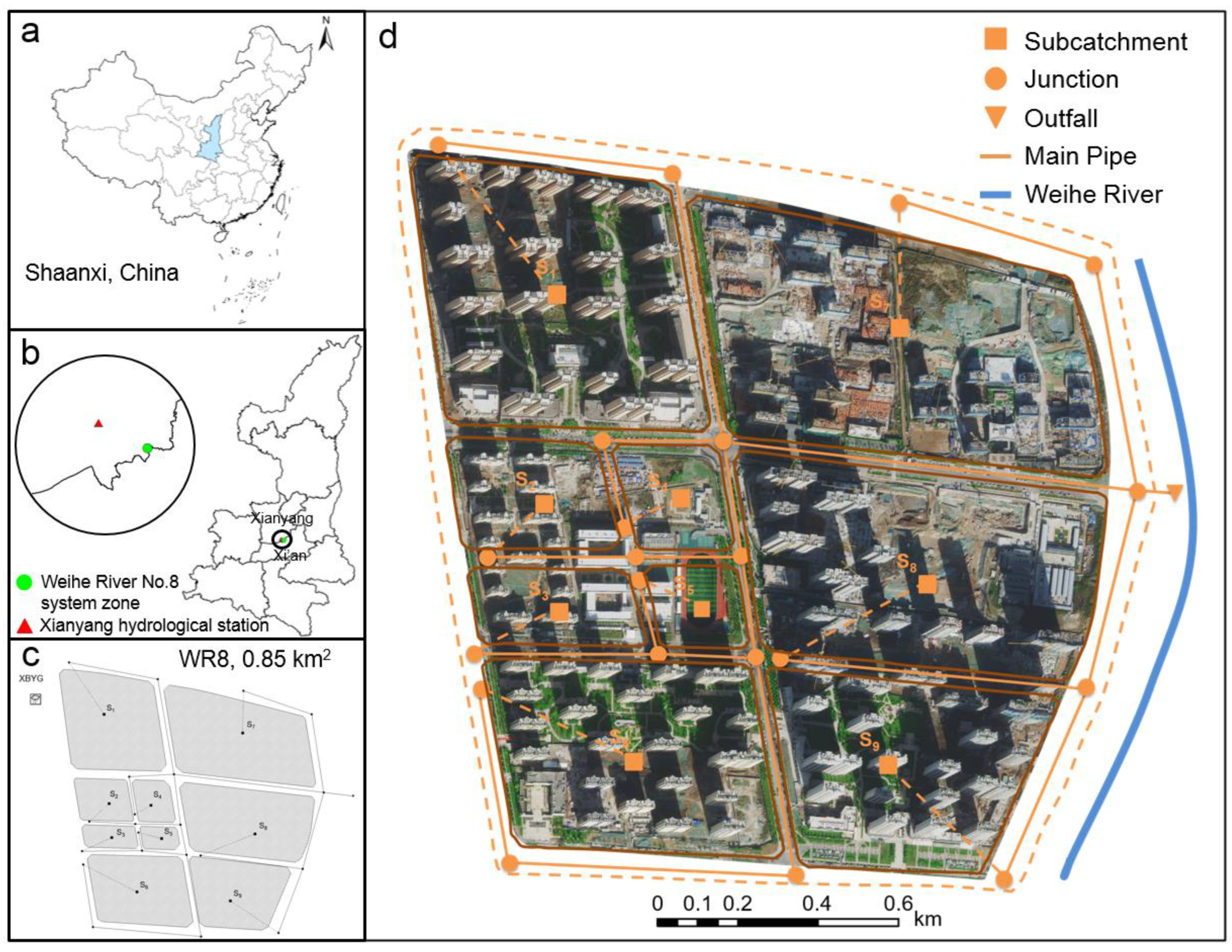
The Weihe River No.8 system zone (WR8, 0.85 km2, Figure 1) is an urban drainage area in Fengxi New City, a designated UNESCO Ecohydrology demo site [34] and a pilot sponge city in China. Many LIDs, such as green roofs, permeable pavements, and bioretention cells, have been built since 2013 to improve the stormwater management infrastructure. WR8 has an elevation of 380.5–384.3 m and covers a layer of non-self-weight collapsible loess. The stormwaters in WR8 are drained to the Fenghe River through the outfall in Figure 1d. The main types of land cover use are residential, educational, and transportation land. It is situated in a warm temperate zone with a continental monsoon semi-arid and semi-humid climate. The annual average precipitation is 552.0 mm, and the rainfall is uneven throughout the year. The precipitations are primarily concentrated in the wet seasons, i.e., from July to September, (accounting for 50–60% of the annual total). We obtained most of the data for applying the storm water management model (SWMM) [35] from the Fengxi Management Committee [36]. In addition, we collected the rainfall time series of 2000 and 2002–2017 at the Xianyang hydrological station (Figure 1c) from the Xi’an University of Technology [37].
3. Methodology
3.1. Event-Based Stochastic Parametric Rainfall Simulator (ESPRS)
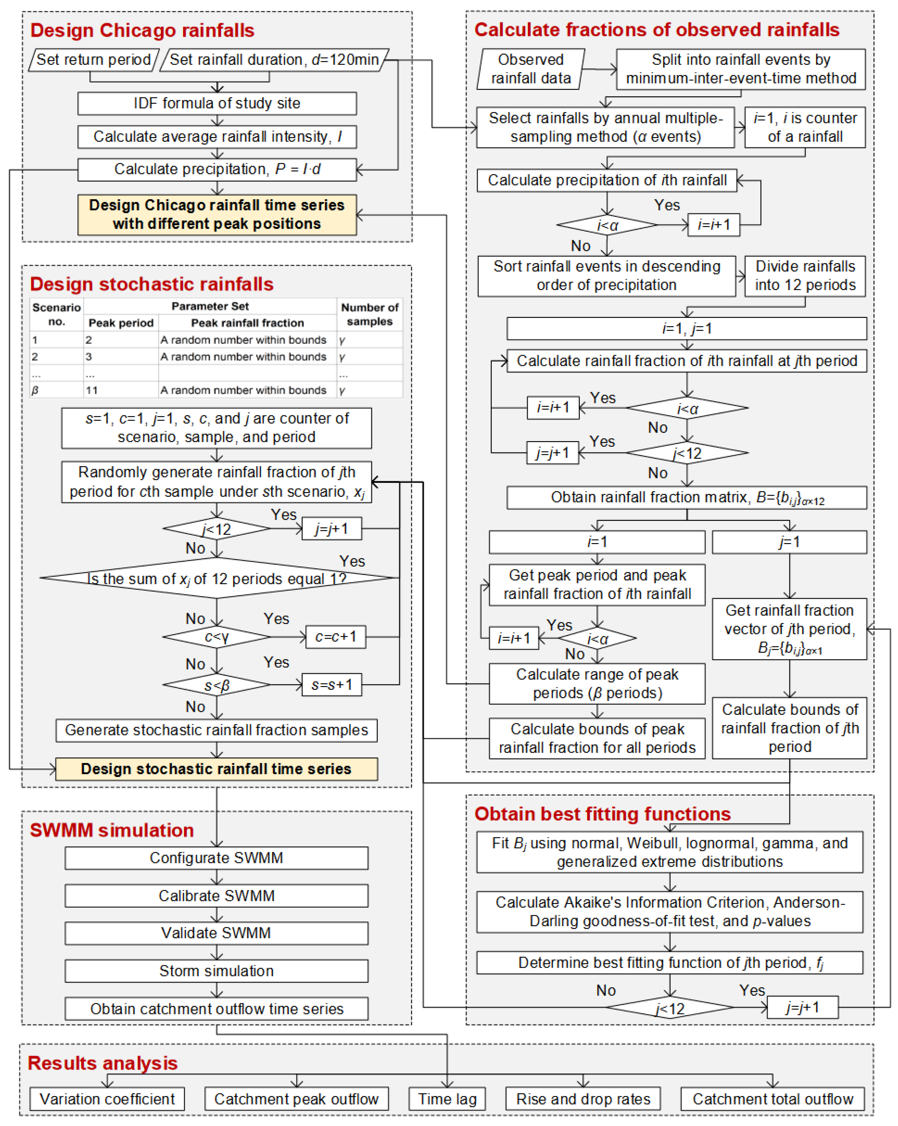
We define the rainfall fraction (RF) as the ratio of rainfall depth in a period to the total precipitation for a rainfall event. The framework of the ESPRS (Figure 2) consists of four steps: (1) Divide the measured rainfall data into events using the minimum interval time method, select the rainfall events using the annual multiple-sampling method, and sort the rainfall events in descending order of precipitation. (2) Equally divide the rainfall events into 12 periods and calculate the RF matrix, the bounds of the RF of each period, and the peak RF. (3) Fit each period’s RF using five probability density functions (PDFs) and determine the PDFs’ best formulas and parameters based on the Akaike’s Information Criterion, Anderson—Darling goodness-of-fit test, and p-values. (4) Set two parameter scenarios, generate the stochastic rainfall patterns (RFs), and distribute the precipitation with the rainfall patterns to calculate the stochastic rainfall time series.
3.1.1. Rainfall Fractions (RFs)
First, we split the collected rainfall time series into events using the minimum inter-event time method [38]. Then, we selected the rainfall events with durations of 120 min and precipitation greater than 2 mm using the annual multiple-sampling method. Thus, we obtained a total of 37 measured rainfall time series. Third, we sorted these events in descending order of the total precipitation and used them to generate time series with 10 min intervals using linear interpolation. Finally, we calculated the RFs of the observed rainfall events as follows:
where pi,j is the rainfall depth in the jth period for the ith rainfall event, mm; and bi,j is the ratio of precipitation in the jth period to the total precipitation for the ith rainfall event. The RF matrix for α measured precipitation events is expressed as
where α is the number of rainfall events. Thus, the RF of the jth period is
3.1.2. Probability Distribution Functions (PDFs)
When choosing a PDF for a parametric rainfall model to describe the probability distribution, the domain of definition, curve flexibility, and simplicity of the function should be deliberated [39]. The normal (denoted as N), Weibull (denoted as W), lognormal (denoted as L), gamma (denoted as G), and GEV (denoted as E) distribution functions [30] were used to fit the observed RFs of each period using the maximum likelihood function. More specifically, the parameters of each PDF are the maximum likelihood estimates.
where x are the RFs for a given period, i.e., Bj; μ, σ, and ξ are the parameters of a PDF, which need to be estimated. Thus, we obtained 60 fitting functions (12 periods, each with 5 functions).
3.1.3. Goodness-of-Fit Statistics
We calculated the Akaike’s Information Criterion (AIC), Anderson—Darling test (AD), and p-values of each fitting function to examine the goodness-of-fit statistics. We namely used the above three criteria to evaluate the agreement of the measured samples to each theoretical distribution.
A smaller value of AIC represents a better fitting [40]:
where α is the number of sample points (i.e., the number of measured rainfall events); and xi are the theoretical and empirical frequency values of the ith sample, respectively; and k is the number of parameters of a PDF that needs to be estimated, which are 2, 2, 2, 2, and 1, respectively (see Equations (4)–(8)).
We performed the AD test and obtained the statistic (a smaller one indicates a better fit) to measure the distance between the theoretical and empirical distributions.
where Yi is the value of the ith sample point (note that the samples were sorted in ascending order); and F is the cumulative distribution function of the target distribution.
The p-value for a significance test represents the probability that the fitted value of a probabilistic model is greater than or equal to the measured data. A p-value greater than 0.05 (i.e., the significance level) indicates that the data obey the target distribution; otherwise, the data do not follow the target distribution.
where c1, c2, c3, c4, and c5 are coefficients determined by .
3.1.4. Stochastic Rainfall Fraction Series
We used the best distribution functions of each period to randomly generate a 12-by-1 vector to represent the RFs of a simulated rainfall event. The stochastic RF series should satisfy the following constraints: (1) Each RF should be within the lower and upper limits of the measured RF for the jth period (i.e., yellow polygon block in Figure 3).
(2) The sum of the RFs should be 1.
(3) The peak RF should be within the lower and upper limits of the measured peak RF. The peaks of the measured precipitation events are in the 2–11 periods (see Figure 3), so we let the rainfall peak at the pth period (j = 2, 3, …, 11):
where Sp is the set of measured rainfall events that peak at the pth period.
3.1.5. Stochastic and Chicago Rainfall Time Series
The average intensity (i, mm/min) of the rainfall in WR8 was calculated using the intensity—duration—frequency formula:
where T and d are the return period and duration, respectively. Here, T = 2 yr and d = 120 min. The precipitation (P, mm) was calculated as follows:
Finally, multiplying the precipitation with the RF series generated the stochastic rainfall time series:
Meanwhile, we used the Chicago method [20] to design ten events of 2-year, 120 min storms with peak periods ranging from 2 to 11 for comparing the catchment outflows.
3.2. Storm Water Management Model (SWMM)
The United States Environmental Protection Agency developed the SWMM in 1971. The software includes hydrological, hydraulic, and water quality modules and is freely used worldwide. To execute the model and facilitate a runoff simulation under vast precipitation events simulated in MATLAB [41], we used MatSWMM [42] because this tool is an open-source MATLAB version developed on the SWMM engine. We have executed a calibrated SWMM in WR8 many times; for more details, such as the parameters, please refer to study [1].
3.3. Performance Evaluation
We set ten scenarios, each generating 1000 stochastic rainfall samples (i.e., γ = 1000). Thus, 10 × β randomized rainfall time series were generated. The rainfall time series were input into SWMM to simulate the outflow time series of the catchment.
We used the variation coefficient (CV) to quantify the changes in the variability of the rainfall time series and the catchment’s corresponding outflow time series. A higher CV represents a more uneven temporal distribution.
where X(t) is the rainfall (or outflow) time series; and t and n are the number and length of the time series, respectively.
To distinguish the flow characteristics, we used six indicators, namely the peak rate (Qm), peak time (tm), flood duration (tD), variation coefficient (QCV), flood rise rate (Qr), and flood drop rate (Qd).
where Q(t) is the flow time series with a length of N, m3/s; and Q0 and Qend are the flow rate at the onset time (t0) and end time (tend) of the flood, respectively.
We also calculated each rainfall event’s lag time, which is the difference between the outflow and rainfall peak moments:
where tr and tp are the lag time and rainfall peak time, respectively. The tp of stochastic precipitation events approximately equals the peak period’s middle moment.
4. Results and Discussion
4.1. Stochastic Rainfall Fractions
Figure 3 depicts the RFs of 12 periods (1–12) and peak RFs of 10 periods (2–11) for the 37 measured precipitation events. We selected the best-fitting PDFs of different periods based on the results of AIC, , and p-value.
Table 1 presents five PDF performances for the first period’s RF. For the first period, the AIC and of the lognormal distribution were the smallest, and the p-value exceeded 0.05. Thus, the lognormal distribution was best for this period. Likewise, the best PDFs of the 2–12 periods were determined in Table 2.
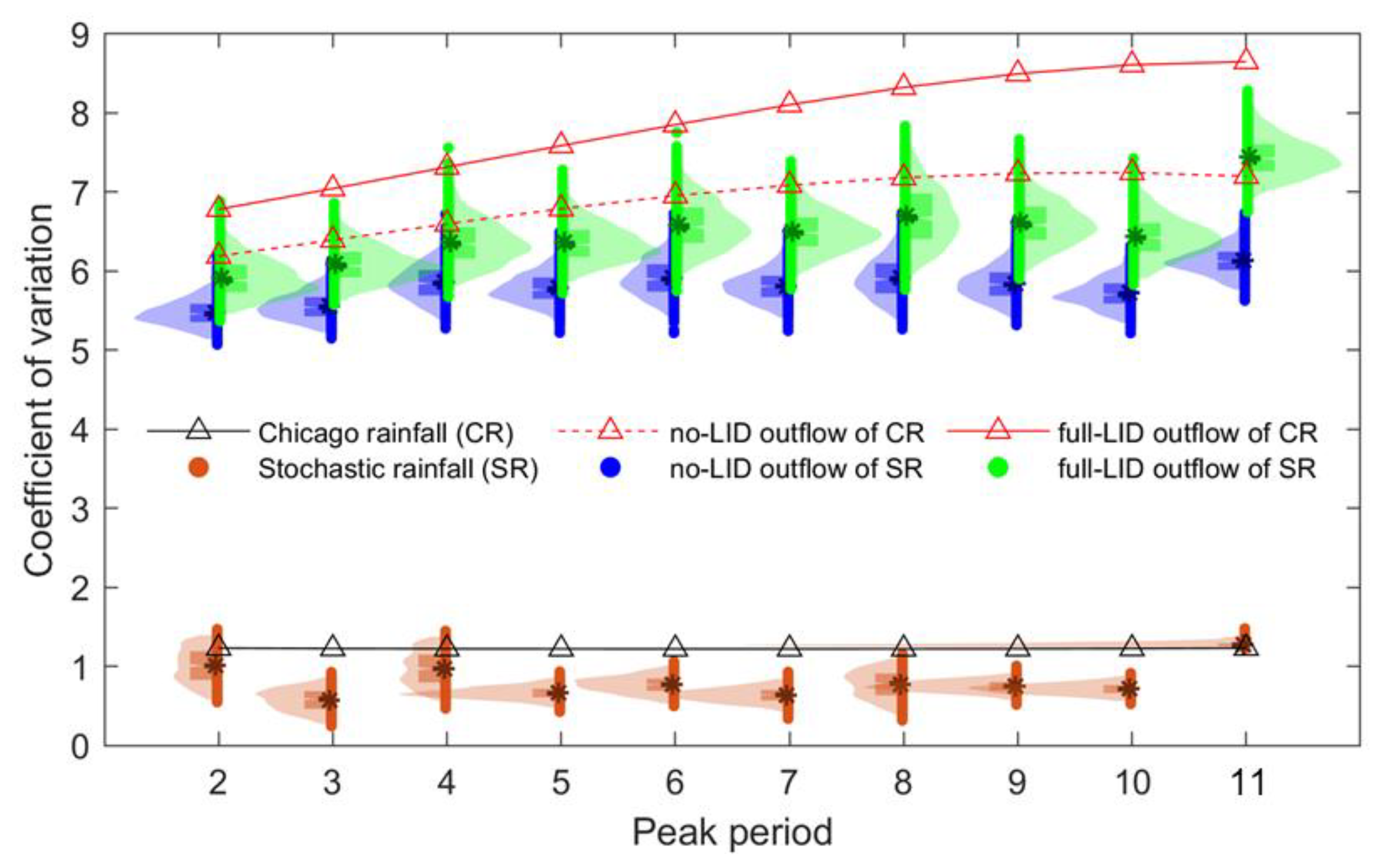
The peak rainfall fraction is a crucial factor for the ESPRS. Figure 4 provides the RFs and catchment outflow time series. These RF curves show that the patterns were sharper and more unimodal when the rainfall had a bigger peak fraction (i.e., when the peak periods were 2, 4, 8, and 11). The peak RFs of the most stochastic precipitation events were lower than those of the Chicago precipitation events. The CVs of the precipitation events generated using the ESPRS correlate with the peak RFs. Figure 5 presents the CVs of the rainfall and outflow time series. For the Chicago precipitation events, the CVs stayed within 1.22–1.23 for all peak periods, suggesting that the peak position hardly impacts the dispersion of the time series; for the stochastic precipitation events, the CVs had a positive correlation with the peak RFs. The CVs of most stochastic precipitation events exceeded those of the Chicago precipitation events. There were exceptions when the rainfall peak period was 2, 4, or 11 because the RFs of these periods had significant upper limits (0.44, 0.43, and 0.40, respectively).
4.2. Catchment Outflow
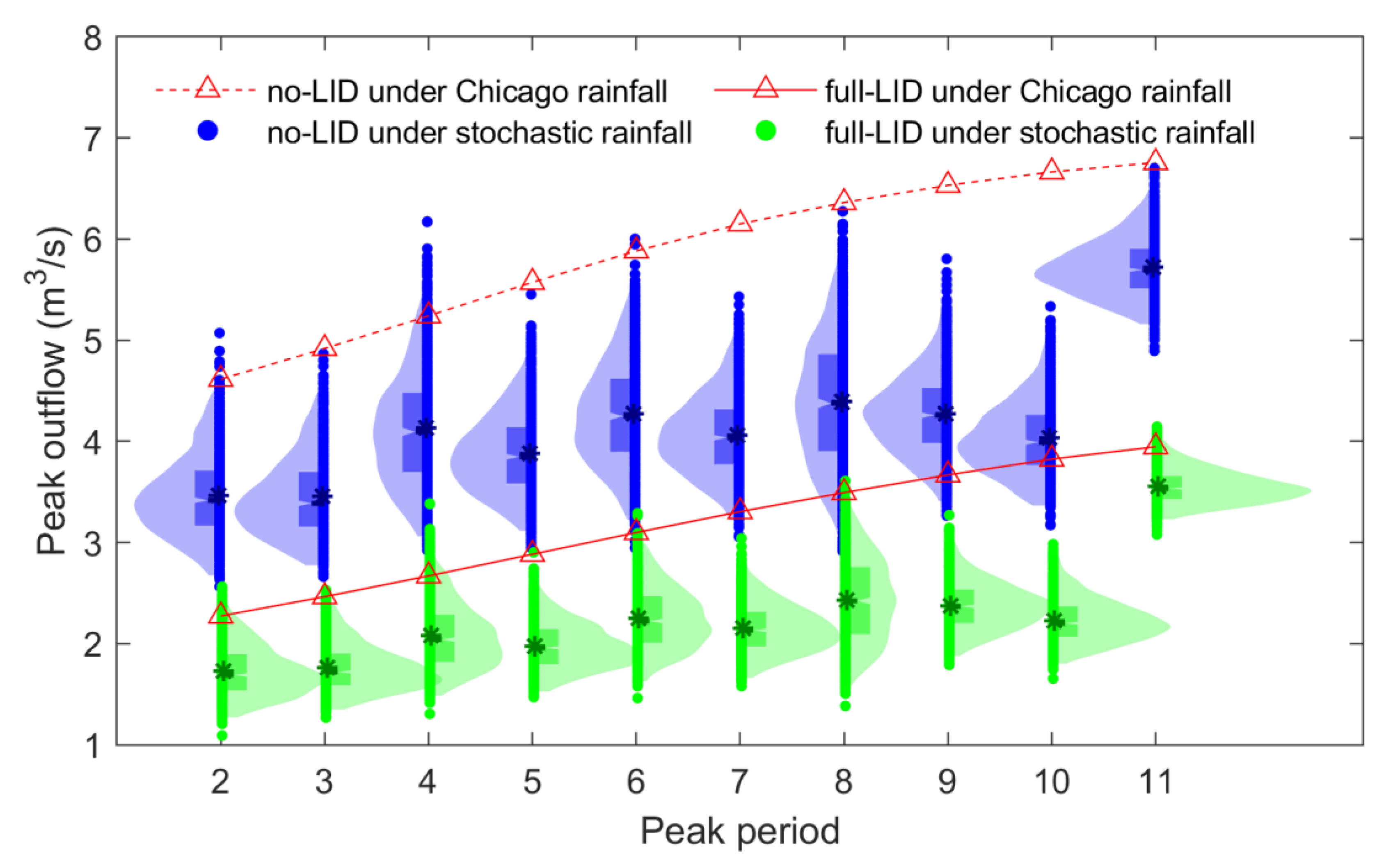
The rainfall peak period and its cumulative depth are critical factors for the ESPRS as they influence the outflow peaks. As the rainfall peak period increased, the outflow peak rate and time under most precipitation events increased (as shown in Figure 4). For a given peak period, the outflow peak time under most stochastic precipitation events exceeded those under Chicago precipitation events; however, exceptions occurred in cases where the cumulative depth at the peak period exceeded that of a Chicago rainfall. The outflow CVs were higher than rainfall CVs because of the underlying surface (as shown in Figure 5). The outflow CVs increased as the rainfall periods increased; however, they did not correlate with the rainfall CVs or peak RFs. Figure 5 demonstrated that the outflow CVs in the full-LID scenario displayed a more widely dispersed distribution than that in the no-LID scenario, indicating a greater diversity of outflow rates following the implementation of LIDs under stochastic precipitation events. Figure 6 shows the catchment peak outflow rate in no-LID and full-LID scenarios under the Chicago and stochastic precipitation events. The peak outflow rates increased as the rainfall peak periods increased and did not correlate with peak RF under most stochastic precipitation events. For a given rainfall peak period, the outflow peak rates under most stochastic precipitation events were less than that under the Chicago rainfall, suggesting that the Chicago precipitation events probably caused an overestimation. Exceptions occurred when the peak RF of a stochastic rainfall exceeded that of the Chicago rainfall or when the cumulative rainfall at the peak period was greater than that of the Chicago rainfall. Furthermore, the peak outflow rates in the full-LID scenario exhibited a more concentrated distribution than that in the no-LID scenario under stochastic precipitation events, indicating a reduction in the diversity of peak outflow rates.
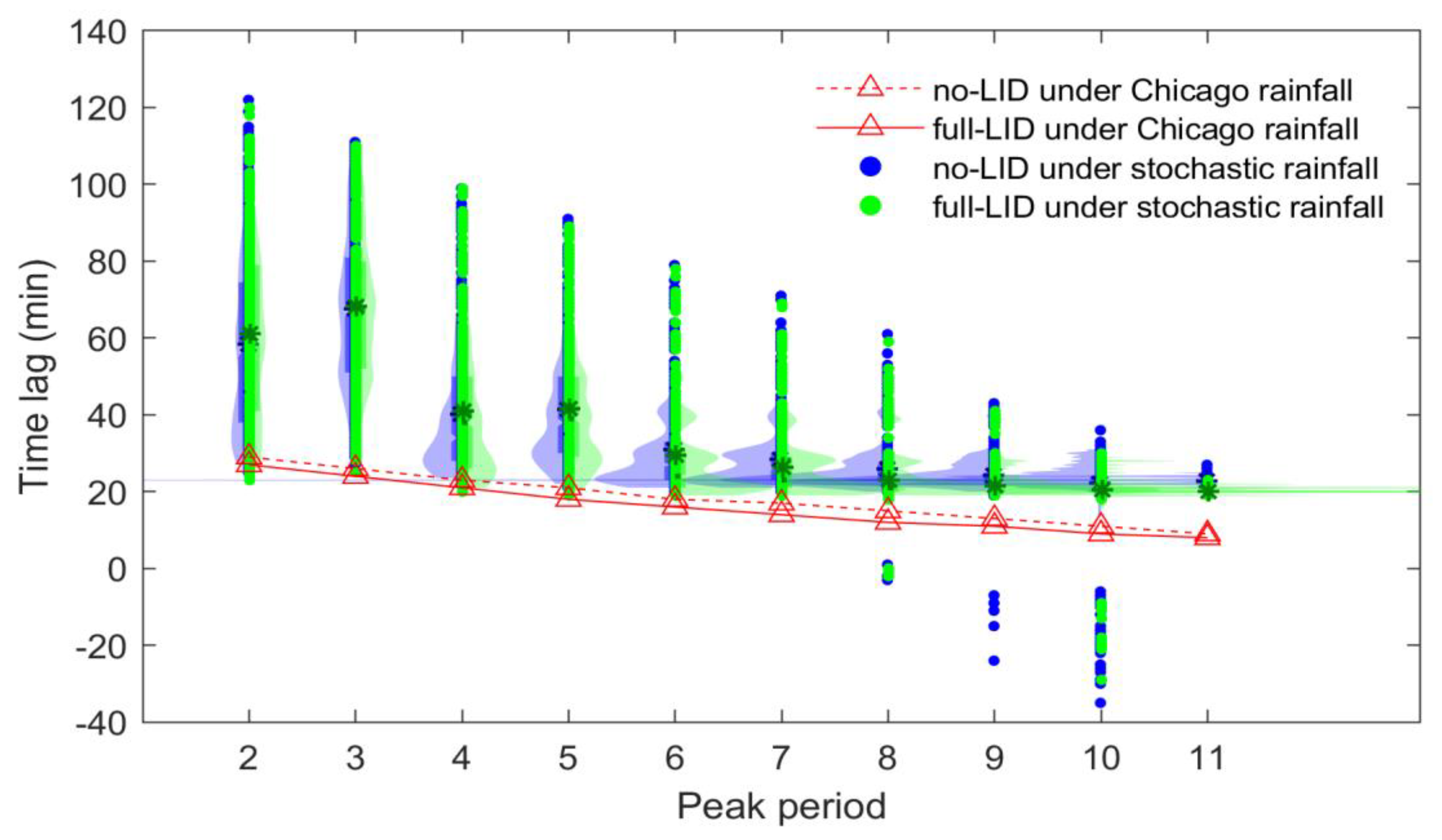
The rainfall peak period and its cumulative depth significantly influence the time lag, which refers to the lag of the peak moment between outflow and rainfall. Figure 7 shows a gradual decrease in the time lags as the rainfall peak period increases. The result might be explained by the fact that the soil moisture contents at the rainfall peak moment were higher under precipitation events with a larger peak period, so the run-off and outflow rose earlier. For a given peak period, the time lag under most stochastic precipitation events exceeded that under Chicago precipitation events, suggesting that the Chicago patterns were a high-risk pattern compared to most stochastic patterns. Exceptions included some stochastic precipitation events with peak periods of 2, 4, 5, and 8–10. We analyzed these stochastic precipitation events’ RFs and outflows and determined that their cumulative RFs at the rainfall peak period exceeded that of the Chicago precipitation events. The lag time under a few stochastic precipitation events with a peak period of 8–10 turned negative. ore specifically, their peak time of outflow occurred earlier than that of rainfall. Further analysis showed that their outflow CV values were small (most had bimodal peaks), and the cumulative RFs at the rainfall peak period were above 0.74, 0.89, and 0.90, respectively. In addition, the time lag in the full-LID scenario exhibited a more concentrated distribution with increasing rainfall peak periods under stochastic precipitation events. This can be attributed to the concentration of outflow peak time as the rainfall peak period increased.
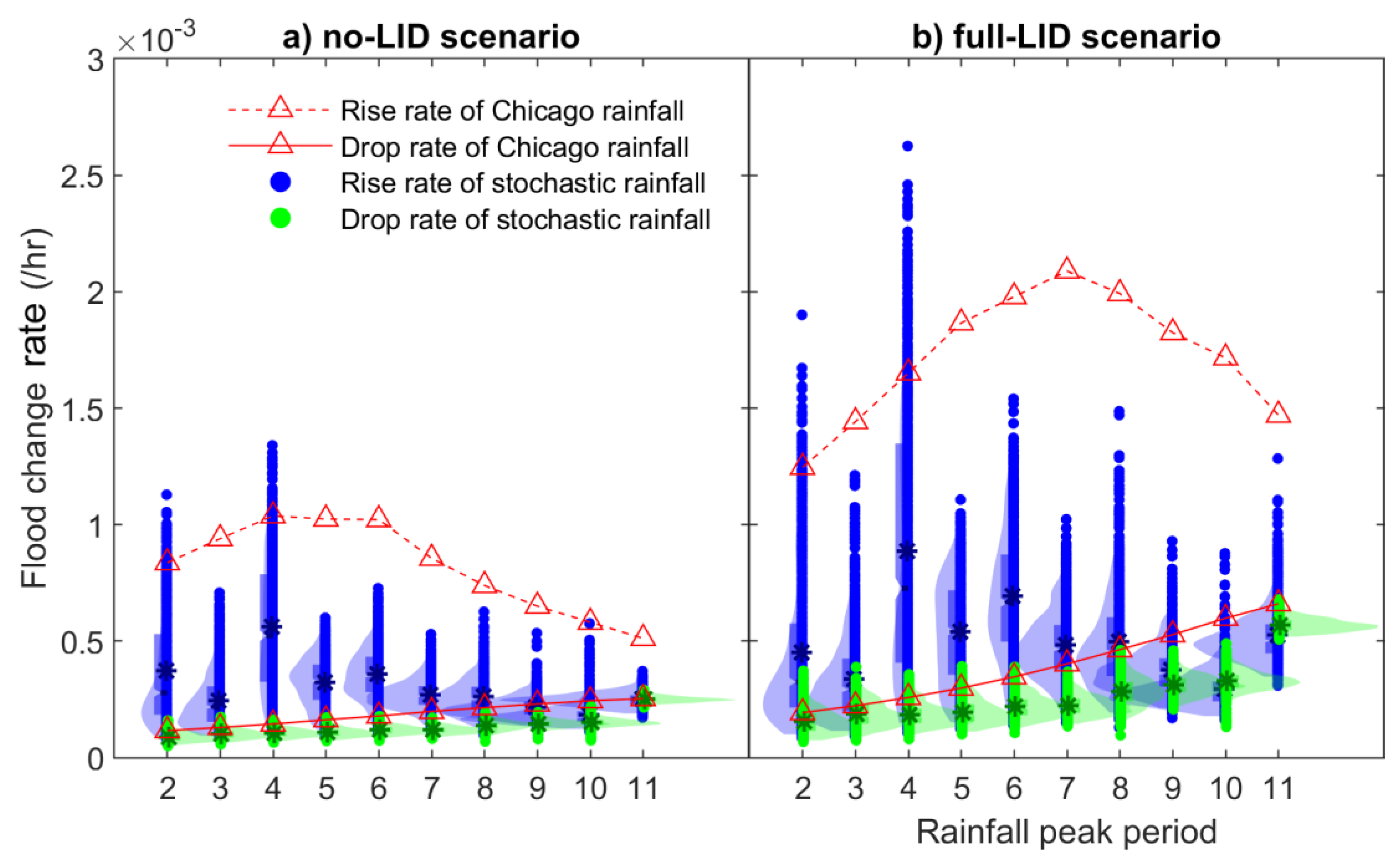
The rise and drop rates of the flood time series under most stochastic precipitation events correlate with the rainfall peak period and peak fraction. Figure 8 presents the rise and drop rates in the no-LID and full-LID scenarios under the Chicago and stochastic precipitation events. As the peak period of the stochastic rainfall increased, the rise rates in the two scenarios increased and then decreased, reaching the maximum when the peak period was four. This trend was consistent with the change in the upper and lower limits of the peak RF in Figure 3. The rise rate positively correlated with the peak RF for precipitation events with a peak period of 2–9, where the correlation coefficients in the non-LID and full-LID scenarios were 0.09–0.74 and 0.12–0.64, respectively. The rise rates under stochastic precipitation events with a peak period of two and four had a wide range due to the wide range of peak RFs. Under two types of precipitation events, the flood drop rates monotonically increased as the peak periods increased and they correlated with the peak RF. For a given peak period, the rise and drop rates under most stochastic precipitation events were lower than those of the Chicago precipitation events, but exceptions existed. Under most stochastic precipitation events, floods were the front type as the rise rates exceeded the corresponding drop rates. The rear-type floods occurred under the stochastic precipitation events with late or small peak periods, but most precipitations dropped after the peak time. We also determined that the drop rates displayed a more concentrated distribution than the rise rate under stochastic precipitation events.
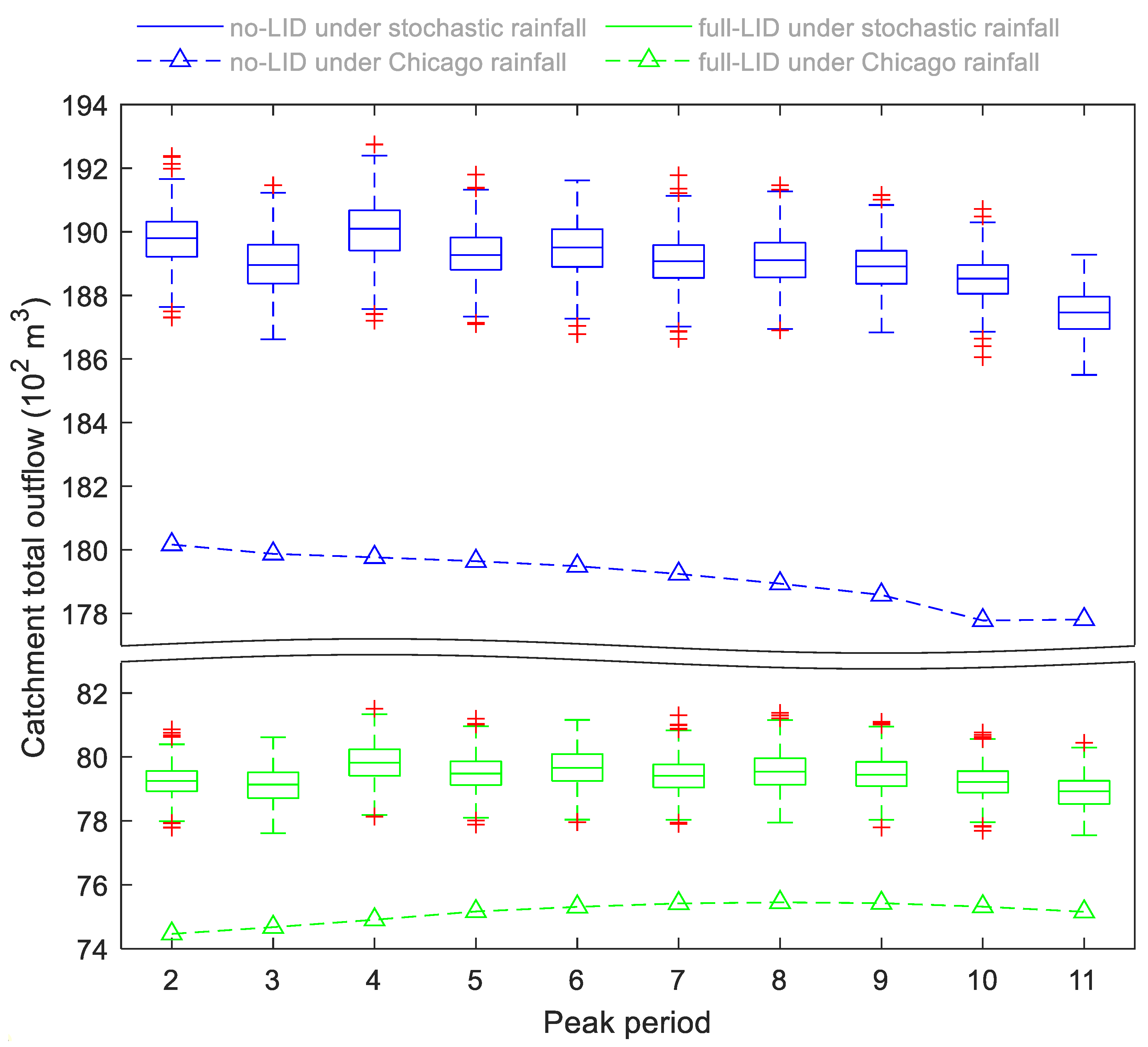
As shown in Figure 9, the catchment total outflow in no-LID and full-LID scenarios under the Chicago and stochastic precipitation events had minor variances. For a given peak period, the total outflow under stochastic precipitation events exceeded that under the Chicago rainfall. We also conducted a correlation analysis and determined that the total outflow did not correlate with the rainfall peak period and peak RF. Its reduction rates remained at 57.45–58.67% under the two types of precipitation events.
4.3. Low-Impact Development Facilities
The flood peaks with LIDs in the study site were earlier than those without LIDs because they could effectively reduce the catchment outflow (peak rate and volume). The outflow peak rates decreased under most precipitation events after constructing the LIDs, which is common sense; interestingly, so did the outflow peak time (Figure 4). Under the Chicago precipitation events, the outflows peaked 1–3 min early after constructing the LIDs; a similar effect was also observed under most of the stochastic precipitation events. On the other hand, the LIDs could cause the study site to approach the pre-development status, i.e., with a more natural hydrological response. The outflow CV in the full-LID scenario exceeded that in the no-LID scenario under a given rainfall, and the outflow CV differences between the two scenarios grew as the rainfall peak period increased (Figure 5).
5. Conclusions
We proposed and validated the ESPRS in a sponge city. We demonstrated that an ESPRS can quickly generate vast, reliable stochastic rainfall time series for an urban hydrologic simulation based on a few measured data while retaining the statistical characteristics of measured precipitation events. Using the vast stochastic precipitation events with different temporal structures generated using the ESPRS to run SWMM, we revealed and summarized the pattern of the catchment outflow in no- and full-ID scenarios. We believe that using an ESPRS will support exemplary urban stormwater management. We conclude that:
- The ESPRS outperformed the Chicago method in predicting extreme precipitation events for urban stormwater simulation and control. Fixed rain patterns can hardly represent the actual temporal structures of precipitation events, especially the extreme ones, leading to uncertainties. Using an ESPRS has strong potential for revealing the influence of temporal rainfall characteristics on hydrological responses.
- The rainfall peak period, rainfall peak fraction, and cumulative rainfall depth at the peak period are control factors for an ESPRS.
- Rear-type precipitation events with high peak fractions present the most negative pattern for outflow control by LIDs.
This study demonstrates that the ESPRS excelled in designing precipitation events. Future studies can be focused on (1) theoretically evaluating the rationality of assuming that rainfall event RFs are independent of each other and quantifying the data of measured rainfall time series for estimating parameters of a PDF; (2) combination with physical-based rainfall models since rainfall is deterministic and stochastic; and (3) investigating the ways in which the temporal variability of rainfall affects the hydrological response, as well as conducting the spatial decomposition of precipitation events based on the spatial heterogeneity.
Author Contributions
Conceptualization, Y.Y.; methodology, Y.Y.; software, Y.Y. and X.X.; validation, Y.Y. and X.X.; formal analysis, Y.Y.; investigation, X.X.; resources, D.L.; data curation, X.X.; writing—original draft preparation, Y.Y.; writing—review and editing, Y.Y. and D.L.; visualization, X.X. and D.L.; supervision, Y.Y.; project administration, Y.Y.; funding acquisition, Y.Y. and D.L. All authors have read and agreed to the published version of the manuscript.
Funding
This work was jointly funded by the National Natural Science Foundation of China (52009099 and 52279025), the China Postdoctoral Science Foundation Funded Project (2019M653882XB), and Shaanxi Provincial Department of Education Funded Project (18JS074). The APC was funded by the Joint Institute of the Internet of Water and Digital Water Governance (sklhse-2019-Iow06).
Data Availability Statement
Not applicable.
Acknowledgments
We thank the editors and reviewers for their helpful comments and suggestions.
Conflicts of Interest
The authors declare no conflict of interest.
References
- Yang, Y.Y.; Li, Y.B.; Huang, Q.; Xia, J.; Li, J.K. Surrogate-based multiobjective optimization to rapidly size low impact development practices for outflow capture. J. Hydrol. 2023, 616, 128848. [Google Scholar] [CrossRef]
- Zhao, Y.M.; Xu, K.; Dong, N.P.; Wang, H. Optimally integrating multi-source products for improving long series precipitation precision by using machine learning methods. J. Hydrol. 2022, 609, 127707. [Google Scholar] [CrossRef]
- Cristiano, E.; ten Veldhuis, M.C.; van De Giesen, N. Spatial and temporal variability of rainfall and their effects on hydrological response in urban areas—A review. Hydrol. Earth Syst. Sci. 2017, 21, 3859–3878. [Google Scholar] [CrossRef]
- Ten Veldhuis, M.-C.; Zhou, Z.; Yang, L.; Liu, S.; Smith, J. The role of storm scale, position and movement in controlling urban flood response. Hydrol. Earth Syst. Sci. 2018, 22, 417–436. [Google Scholar] [CrossRef]
- Zhou, Z.; Smith, J.A.; Wright, D.B.; Baeck, M.L.; Yang, L.; Liu, S. Storm Catalog-Based Analysis of Rainfall Heterogeneity and Frequency in a Complex Terrain. Water Resour. Res. 2019, 55, 1871–1889. [Google Scholar] [CrossRef]
- Wright, D.B.; Yu, G.; England, J.F. Six decades of rainfall and flood frequency analysis using stochastic storm transposition: Review, progress, and prospects. J. Hydrol. 2020, 585, 124816. [Google Scholar] [CrossRef]
- Bruni, G.; Reinoso, R.; van de Giesen, N.C.; Clemens, F.H.L.R.; ten Veldhuis, J.A.E. On the sensitivity of urban hydrodynamic modelling to rainfall spatial and temporal resolution. Hydrol. Earth Syst. Sci. 2015, 19, 691–709. [Google Scholar] [CrossRef]
- Cristiano, E.; ten Veldhuis, M.-c.; Wright, D.B.; Smith, J.A.; van de Giesen, N. The Influence of Rainfall and Catchment Critical Scales on Urban Hydrological Response Sensitivity. Water Resour. Res. 2019, 55, 3375–3390. [Google Scholar] [CrossRef]
- Ochoa-Rodriguez, S.; Wang, L.P.; Gires, A.; Pina, R.D.; Reinoso-Rondinel, R.; Bruni, G.; Ichiba, A.; Gaitan, S.; Cristiano, E.; van Assel, J.; et al. Impact of spatial and temporal resolution of rainfall inputs on urban hydrodynamic modelling outputs: A multi-catchment investigation. J. Hydrol. 2015, 531, 389–407. [Google Scholar] [CrossRef]
- Paschalis, A.; Fatichi, S.; Molnar, P.; Rimkus, S.; Burlando, P. On the effects of small scale space-time variability of rainfall on basin flood response. J. Hydrol. 2014, 514, 313–327. [Google Scholar] [CrossRef]
- Nerini, D.; Besic, N.; Sideris, I.; Germann, U.; Foresti, L. A non-stationary stochastic ensemble generator for radar rainfall fields based on the short-space Fourier transform. Hydrol. Earth Syst. Sci. 2017, 21, 2777–2797. [Google Scholar] [CrossRef]
- Akil, N.; Artigue, G.; Savary, M.; Johannet, A.; Vinches, M. Uncertainty Estimation in Hydrogeological Forecasting with Neural Networks: Impact of Spatial Distribution of Rainfalls and Random Initialization of the Model. Water 2021, 13, 1690. [Google Scholar] [CrossRef]
- Wang, Y.T.; Xie, J.K.; You, Y.F.; Wang, Y.J.; Xu, Y.P.; Guo, Y.X. A new multi-site multi-variable stochastic model with inter-site and inter-variable correlations, low frequency attributes and stochasticity: A case study in the lower Yellow River basin. J. Hydrol. 2021, 599, 126365. [Google Scholar] [CrossRef]
- Yan, J.; Li, F.; Bárdossy, A.; Tao, T. Conditional simulation of spatial rainfall fields using random mixing: A study that implements full control over the stochastic process. Hydrol. Earth Syst. Sci. 2021, 25, 3819–3835. [Google Scholar] [CrossRef]
- Gao, C.; Guan, X.J.; Booij, M.J.; Meng, Y.; Xu, Y.P. A new framework for a multi-site stochastic daily rainfall model: Coupling a univariate Markov chain model with a multi-site rainfall event model. J. Hydrol. 2021, 598, 126478. [Google Scholar] [CrossRef]
- Papalexiou, S.M.; Serinaldi, F. Random Fields Simplified: Preserving Marginal Distributions, Correlations, and Intermittency, With Applications From Rainfall to Humidity. Water Resour. Res. 2020, 56, e2019WR026331. [Google Scholar] [CrossRef]
- Peleg, N.; Blumensaat, F.; Molnar, P.; Fatichi, S.; Burlando, P. Partitioning the impacts of spatial and climatological rainfall variability in urban drainage modeling. Hydrol. Earth Syst. Sci. 2017, 21, 1559–1572. [Google Scholar] [CrossRef]
- Zhu, Z.; Wright, D.B.; Yu, G. The Impact of Rainfall Space-Time Structure in Flood Frequency Analysis. Water Resour. Res. 2018, 54, 8983–8998. [Google Scholar] [CrossRef]
- Hettiarachchi, S.; Wasko, C.; Sharma, A. Increase in flood risk resulting from climate change in a developed urban watershed—The role of storm temporal patterns. Hydrol. Earth Syst. Sci. 2018, 22, 2041–2056. [Google Scholar] [CrossRef]
- Yang, Y.Y.; Li, J.; Huang, Q.; Xia, J.; Li, J.K.; Liu, D.F.; Tan, Q.T. Performance assessment of sponge city infrastructure on stormwater outflows using isochrone and SWMM models. J. Hydrol. 2021, 597, 126151. [Google Scholar] [CrossRef]
- Nguyen, N.S.; Liu, J.; Raghavan, S.V.; Liong, S.-Y. Deriving high spatiotemporal rainfall information over Singapore through dynamic-stochastic modelling using ‘HiDRUS’. Stoch. Environ. Res. Risk Assess. 2020, 35, 1453–1462. [Google Scholar] [CrossRef]
- Pons, V.; Benestad, R.; Sivertsen, E.; Muthanna, T.M.; Bertrand-Krajewski, J.L. Forecasting green roof detention performance by temporal downscaling of precipitation time-series projections. Hydrol. Earth Syst. Sci. 2022, 26, 2855–2874. [Google Scholar] [CrossRef]
- Müller, H.; Haberlandt, U. Temporal rainfall disaggregation using a multiplicative cascade model for spatial application in urban hydrology. J. Hydrol. 2018, 556, 847–864. [Google Scholar] [CrossRef]
- Gao, C.; Booij, M.J.; Xu, Y.P. Development and hydrometeorological evaluation of a new stochastic daily rainfall model: Coupling Markov chain with rainfall event model. J. Hydrol. 2020, 589, 125337. [Google Scholar] [CrossRef]
- Yang, L.; Zhong, P.-a.; Zhu, F.; Ma, Y.; Wang, H.; Li, J.; Xu, C. A comparison of the reproducibility of regional precipitation properties simulated respectively by weather generators and stochastic simulation methods. Stoch. Environ. Res. Risk Assess. 2021, 36, 495–509. [Google Scholar] [CrossRef]
- Kim, D.; Onof, C. A stochastic rainfall model that can reproduce important rainfall properties across the timescales from several minutes to a decade. J. Hydrol. 2020, 589, 125150. [Google Scholar] [CrossRef]
- Mosthaf, T.; Bárdossy, A. Regionalizing nonparametric models of precipitation amounts on different temporal scales. Hydrol. Earth Syst. Sci. 2017, 21, 2463–2481. [Google Scholar] [CrossRef]
- Balbastre-Soldevila, R.; García-Bartual, R.; Andrés-Doménech, I. Estimation of the G2P Design Storm from a Rainfall Convectivity Index. Water 2021, 13, 1943. [Google Scholar] [CrossRef]
- Shmilovitz, Y.; Marra, F.; Wei, H.; Argaman, E.; Nearing, M.; Goodrich, D.; Assouline, S.; Morin, E. Frequency analysis of storm-scale soil erosion and characterization of extreme erosive events by linking the DWEPP model and a stochastic rainfall generator. Sci. Total Environ. 2021, 787, 147609. [Google Scholar] [CrossRef]
- Pavlides, A.; Agou, V.D.; Hristopulos, D.T. Non-parametric kernel-based estimation and simulation of precipitation amount. J. Hydrol. 2022, 612, 127988. [Google Scholar] [CrossRef]
- Zhang, H.; Loáiciga, H.A.; Ren, F.; Du, Q.; Ha, D. Semi-empirical prediction method for monthly precipitation prediction based on environmental factors and comparison with stochastic and machine learning models. Hydrol. Sci. J. 2020, 65, 1928–1942. [Google Scholar] [CrossRef]
- Wang, C.; Hou, J.; Miller, D.; Brown, I.; Jiang, Y. Flood risk management in sponge cities: The role of integrated simulation and 3D visualization. Int. J. Disaster Risk Reduct. 2019, 39, 101139. [Google Scholar] [CrossRef]
- Hou, J.; Mao, H.; Li, J.; Sun, S. Spatial simulation of the ecological processes of stormwater for sponge cities. J. Environ. Manag. 2019, 232, 574–583. [Google Scholar] [CrossRef] [PubMed]
- Fengxi Sponge City (China). Available online: http://ecohydrology-ihp.org/demosites/view/1220 (accessed on 4 March 2023).
- Storm Water Management Model (SWMM). Available online: www.epa.gov/water-research/storm-water-management-model-swmm (accessed on 4 March 2023).
- Fengxi Management Committee. Available online: http://fxxc.xixianxinqu.gov.cn (accessed on 4 March 2023).
- Hou, J.; Guo, K.; Liu, F. Report on Storm Pattern Design and Storm Intensity Formula in Xixian New Area; Xi’an University of Technology: Xi’an, China, 2018. [Google Scholar]
- Pirone, D.; Cimorelli, L.; Del Giudice, G.; Pianese, D. Short-term rainfall forecasting using cumulative precipitation fields from station data: A probabilistic machine learning approach. J. Hydrol. 2023, 617, 128949. [Google Scholar] [CrossRef]
- Papalexiou, S.M. Rainfall Generation Revisited: Introducing CoSMoS-2s and Advancing Copula-Based Intermittent Time Series Modeling. Water Resour. Res. 2022, 58, e2021WR031641. [Google Scholar] [CrossRef]
- Gao, C.; Xu, Y.P.; Zhu, Q.; Bai, Z.X.; Liu, L. Stochastic generation of daily rainfall events: A single-site rainfall model with Copula-based joint simulation of rainfall characteristics and classification and simulation of rainfall patterns. J. Hydrol. 2018, 564, 41–58. [Google Scholar] [CrossRef]
- MATLAB. Available online: https://www.mathworks.com/products/matlab.html (accessed on 4 March 2023).
- Riaño-Briceño, G.; Barreiro-Gomez, J.; Ramirez-Jaime, A.; Quijano, N.; Ocampo-Martinez, C. MatSWMM—An open-source toolbox for designing real-time control of urban drainage systems. Environ. Modell. Softw. 2016, 83, 143–154. [Google Scholar] [CrossRef]
Figure 1.
Map of the study area for simulation: (a) Shannxi Province, China; (b) Weihe River No. 8 system zone (WR8), Fengxi New City; (c) Study area map of WR8 in storm water management model; and (d) Aerial photographs of WR8.
Figure 1.
Map of the study area for simulation: (a) Shannxi Province, China; (b) Weihe River No. 8 system zone (WR8), Fengxi New City; (c) Study area map of WR8 in storm water management model; and (d) Aerial photographs of WR8.

Figure 2.
Event-based stochastic parametric rainfall simulator (ESPRS) framework and storm water management model simulation.
Figure 2.
Event-based stochastic parametric rainfall simulator (ESPRS) framework and storm water management model simulation.

Figure 3.
Rainfall fractions (RF) of 12 periods and their upper and lower limits. For a period, the upper (lower) limit of RF equals the maximum (minimum) value of the measured RFs. For a period, the upper (lower) limit of peak RF means is the maximum (minimum) value of the measured RFs of precipitation events that peaked in that period. The points with different colors represent the fractions of observed rainfalls.

Figure 4.
Rainfall fraction and catchment outflow time series in no- and full-LID scenarios under Chicago and stochastic precipitation events. The no-LID denotes low-impact development facilities (LIDs) are not constructed, and full-LID denotes LIDs are constructed as much as possible.
Figure 4.
Rainfall fraction and catchment outflow time series in no- and full-LID scenarios under Chicago and stochastic precipitation events. The no-LID denotes low-impact development facilities (LIDs) are not constructed, and full-LID denotes LIDs are constructed as much as possible.

Figure 5.
Variation coefficients of Chicago and stochastic rainfall time series and variation coefficients of corresponding outflow time series in no- and full-LID scenarios. * represents the median.
Figure 5.
Variation coefficients of Chicago and stochastic rainfall time series and variation coefficients of corresponding outflow time series in no- and full-LID scenarios. * represents the median.

Figure 6.
Catchment peak outflow rate in no- and full-LID scenarios under Chicago and stochastic precipitation events with different peak periods. * represents the median.
Figure 6.
Catchment peak outflow rate in no- and full-LID scenarios under Chicago and stochastic precipitation events with different peak periods. * represents the median.

Figure 7.
Time lag in no- and full-LID scenarios under Chicago and stochastic precipitation events. * represents the median.
Figure 7.
Time lag in no- and full-LID scenarios under Chicago and stochastic precipitation events. * represents the median.

Figure 8.
Rise and drop rates of flood time series in (a) no- and (b) full-LID scenarios under Chicago and stochastic precipitation events. * represents the median.
Figure 8.
Rise and drop rates of flood time series in (a) no- and (b) full-LID scenarios under Chicago and stochastic precipitation events. * represents the median.

Figure 9.
Catchment total outflow in no- and full-LID scenarios under Chicago and stochastic precipitation events. + represents the outlier.
Figure 9.
Catchment total outflow in no- and full-LID scenarios under Chicago and stochastic precipitation events. + represents the outlier.


Table 1.
Performances of five probability distribution functions for the rainfall fraction of the first period.
Table 1.
Performances of five probability distribution functions for the rainfall fraction of the first period.
| Distribution Function | AIC 1 | p-Value 1 | |
|---|---|---|---|
| Normal | −151.09 | 3.08 | 0.005 |
| Weibull | −191.93 | 1.16 | 0.010 |
| Generalized extreme value | −247.46 | 0.93 | 0.017 |
| Gamma | −198.76 | 0.82 | 0.040 |
| Lognormal | −233.94 | 0.31 | 0.549 |
Note: 1 Smaller values of AIC and represent better fits, and a p-value greater than 0.05 indicates that the data obey the target distribution.
Table 2.
Best-fitting probability distribution functions for 12 periods.
| Period | Best Fitting Form | Formula | Bounds of Rainfall Fraction (x) |
|---|---|---|---|
| 1 | Lognormal | 0.01–0.19 | |
| 2 | Lognormal | 0.01–0.44 | |
| 3 | Gamma | 0.02–0.29 | |
| 4 | Lognormal | 0.03–0.43 | |
| 5 | Gamma | 0.03–0.22 | |
| 6 | Generalized extreme value | 0.02–0.28 | |
| 7 | Gamma | 0.02–0.22 | |
| 8 | Lognormal | 0.02–0.33 | |
| 9 | Generalized extreme value | 0.02–0.23 | |
| 10 | Lognormal | 0.01–0.22 | |
| 11 | Lognormal | 0.01–0.40 | |
| 12 | Lognormal | 0.00–0.13 |
Disclaimer/Publisher’s Note: The statements, opinions and data contained in all publications are solely those of the individual author(s) and contributor(s) and not of MDPI and/or the editor(s). MDPI and/or the editor(s) disclaim responsibility for any injury to people or property resulting from any ideas, methods, instructions or products referred to in the content. |
© 2023 by the authors. Licensee MDPI, Basel, Switzerland. This article is an open access article distributed under the terms and conditions of the Creative Commons Attribution (CC BY) license (https://creativecommons.org/licenses/by/4.0/).
Share and Cite
MDPI and ACS Style
Yang, Y.; Xu, X.; Liu, D. An Event-Based Stochastic Parametric Rainfall Simulator (ESPRS) for Urban Stormwater Simulation and Performance in a Sponge City. Water 2023, 15, 1561. https://doi.org/10.3390/w15081561
AMA Style
Yang Y, Xu X, Liu D. An Event-Based Stochastic Parametric Rainfall Simulator (ESPRS) for Urban Stormwater Simulation and Performance in a Sponge City. Water. 2023; 15(8):1561. https://doi.org/10.3390/w15081561
Chicago/Turabian StyleYang, Yuanyuan, Xiaoyan Xu, and Dengfeng Liu. 2023. "An Event-Based Stochastic Parametric Rainfall Simulator (ESPRS) for Urban Stormwater Simulation and Performance in a Sponge City" Water 15, no. 8: 1561. https://doi.org/10.3390/w15081561
Note that from the first issue of 2016, this journal uses article numbers instead of page numbers. See further details here.