
Research on Rain Pattern Classification Based on Machine Learning: A Case Study in Pi River Basin
by
 ,
,
Xiaodi Fu
1,2,3, 
Guangyuan Kan
1,2,3,*,
Ronghua Liu
1,2,3,
Ke Liang
4,
Xiaoyan He
1,2,3 and
Liuqian Ding
1,2 1
State Key Laboratory of Simulation and Regulation of Water Cycle in River Basin, Beijing 100038, China
2
China Institute of Water Resources and Hydropower Research, Beijing 100038, China
3
Research Center of Flood & Drought Disaster Reduction of the Ministry of Water Resources, Beijing 100038, China
4
Beijing IWHR Corporation, Beijing 100048, China
*
Author to whom correspondence should be addressed.
Water 2023, 15(8), 1570; https://doi.org/10.3390/w15081570
Submission received: 12 March 2023
/
Revised: 11 April 2023
/
Accepted: 15 April 2023
/
Published: 17 April 2023
(This article belongs to the Special Issue Hydrological Simulation and Forecasting Based on Artificial Intelligence)
Abstract
:For the purpose of improving the scientific nature, reliability, and accuracy of flood forecasting, it is an effective and practical way to construct a flood forecasting scheme and carry out real-time forecasting with consideration of different rain patterns. The technique for rain pattern classification is of great significance in the above-mentioned technical roadmap. With the rapid development of artificial intelligence technologies such as machine learning, it is possible and necessary to apply these new methods to assist rain classification applications. In this research, multiple machine learning methods were adopted to study the time-history distribution characteristics and conduct rain pattern classification from observed rainfall time series data. Firstly, the hourly rainfall data between 2003 and 2021 of 37 rain gauge stations in the Pi River Basin were collected to classify rain patterns based on the universally acknowledged dynamic time warping (DTW) algorithm, and the classifications were treated as the benchmark result. After that, four other machine learning methods, including the Decision Tree (DT), Long- and Short-Term Memory (LSTM) neural network, Light Gradient Boosting Machine (LightGBM), and Support Vector Machine (SVM), were specifically selected to establish classification models and the model performances were compared. By adjusting the sampling size, the influence of different sizes on the classification was analyzed. Intercomparison results indicated that LightGBM achieved the highest accuracy and the fastest training speed, the accuracy and F1 score were 98.95% and 98.58%, respectively, and the loss function and accuracy converged quickly after only 20 iterations. LSTM and SVM have satisfactory accuracy but relatively low training efficiency, and DT has fast classification speed but relatively low accuracy. With the increase in the sampling size, classification results became stable and more accurate. Besides the higher accuracy, the training efficiency of the four methods was also improved.
1. Introduction
Rain pattern and intensity are the most commonly used parameters for describing rainfall characteristics and are important factors that affect hydrological processes [1,2], playing a crucial role in the analysis of hydrological, hydraulic, and water quality models. With the increasing sample size of hydro-meteorological data and the continuous development of artificial intelligence technology, the use of machine learning methods to extract important characteristics of rainfall-runoff from large amounts of hydrological data can better identify hydrological regularities [3,4], improve the scientificity and reliability of rainfall classification, and provide powerful technical support for efficient flood forecasting.
Rain pattern is numerically represented by the distribution process of rainfall intensity over a time scale. Early research was based on a statistical analysis of large amounts of measured rainfall data. In 1956, Soviet researchers such as Pakhomova and M.B. Morokov [5] statistically analyzed a large amount of measured rainfall data and summarized seven classic rainfall types, known as model rain patterns. In 1957, Keifer and Chu [6] proposed the Chicago rainfall type. In 1967, Huff [7] divided rainfall into four types based on the different locations of rainfall types in the analysis of storm rainfall types in Illinois, known as the Huff rainfall type. In 1975, Pilgrim and Cordery [8] proposed a generalized rainfall type, using the mean proportional value of hourly rainfall for many years of measured rainfall data as the unit rainfall distribution value, known as the P&C rainfall type. In 1980, Yen and Chow [9] proposed a triangular rainfall type. In 1964, Zhao Guangrong [10] statistically analyzed the heavy rainfall in Guangdong Province and roughly divided it into three types and eight categories. In 1994, Wang Min [11] and others proposed a design storm rainfall type for Beijing based on rainfall data. There are substantial differences between various rainfall types, and currently, there is no unified rainfall type as a design basis.
Rain pattern is one of the most important front-end input data for rainfall-runoff simulation, and it has a significant impact on the simulation results of both rainfall-runoff experimental models, physical mechanism hydrological models, and data-driven hydrological models. Wu Zhangchun et al. [12] found that under the same average rainfall intensity within the runoff duration, the peak of the triangular rain pattern in the middle or at the back was more than 30% higher than that of the uniform rain pattern through indoor simulation of rainfall-runoff experiments. Based on the seven rain patterns proposed by Pakhomova, M.B. Morokov, and others, Cen Guoping [13] used a fuzzy identification method to statistically analyze and classify rain patterns at four precipitation stations and conducted rainfall-runoff experimental studies. The results showed that rain pattern has significant effects on peak flow and flow process lines. Zhao Kangqian [14] classified six rainfall events using model rain patterns, selected 12 parameters that varied within the interval, compared SWMM simulation total runoff and peak variable changes, and analyzed the sensitivity of parameters. The results showed that rain pattern has a significant impact on parameter sensitivity. Zhang Xiaoyuan [15] designed three rain patterns: single peak, double peak, and triple peak for SWMM hydrological parameter sensitivity analysis, and the results showed that rain patterns significantly impacted parameter sensitivity and recognition performance. Tu Xinyu [16] used the constructed HEC-HMS model to simulate peak flow rates corresponding to different rain patterns and fixed total rainfall amounts. The results showed that the peak flow rates simulated for different rain patterns had significant deviations, and rain patterns had a significant impact on rainfall-runoff calculation. Yang Senxiong [17] used seven model rain patterns to perform fuzzy identification and classification on 43 rainfall events and used the SWMM model to predict rainfall-runoff. The results showed that the rainfall-runoff simulation results of different rain patterns had significant differences, indicating that the rain pattern has a significant impact on the generalization performance and accuracy of the model prediction. Based on the characteristics of rain patterns, the DTW hierarchical clustering algorithm was used for rainfall event classification, and the data set was reconstructed based on the classification results. A deep learning model was used to construct an integrated data-driven model for rainfall-runoff prediction, and the prediction results were higher than those without clustering rain patterns, indicating that rain pattern has a significant impact on the prediction performance of rainfall events.
In the process of establishing the relationship between rainfall and runoff, if only one rain pattern is used to represent the comprehensive rainfall distribution process in the area, the diversity of rainfall itself will be ignored. Due to the important role of rainfall patterns in simulating rainfall-runoff, diverse rainfall patterns can avoid homogenization of model parameters, ensuring accurate, precise, and scientific simulation of rainfall runoff in hydrological models. Therefore, it is necessary to conduct a diversity classification study of rainfall patterns in the basin.
Traditional rain pattern classification methods are cumbersome and lack strong visualization, which hinders their application. With the development of machine learning algorithms, cluster analysis is more objective and fully reflects the rainfall process. Gupta et al. [18] used K-means clustering to classify different types of heavy rain patterns in Texas based on the spatial characteristics of hourly rainfall. Gao et al. [19] used K-means clustering analysis to classify and optimize the rain patterns at Dongyang station, dividing them into uniform, late peak, central peak, and early peak types. Yin Shuiqing [20] used the dynamic K-means clustering method to classify rainfall data from 14 meteorological stations in China, dividing the rainfall process into four patterns: early-stage, mid-stage, late-stage, and uniform, based on the rain peak position as the measurement standard. Liu Yuanyuan [21] analyzed the rain patterns in Beijing during the flood season using the DTW method and fuzzy pattern recognition. Hu Rui et al. [22] summarized the rain pattern laws at the Baoji meteorological station in Shaanxi Province using the Ward clustering method in hierarchical clustering. Previous research mostly used DTW-based fuzzy recognition methods and K-means clustering for rainfall pattern clustering, with other AI methods less commonly used in rainfall pattern classification applications. The Long- and Short-Term Memory (LSTM) neural network model can handle long-term memory information and has high model prediction accuracy. Support Vector Machines (SVM) perform well on a small sample and nonlinear problems, with good generalization ability. A Decision Tree (DT) is a tree-like structure that represents a mapping relationship between object attributes and object values. It has a simple structure, can handle massive data, and has a fast computational speed and high classification accuracy. The lightweight gradient boosting machine (LightGBM) in the ensemble learning model has low memory consumption and fast training speed and still has good performance when processing large-scale data.
Although the spatial distribution of rainfall is of great significance, the current study is focused on temporal patterns. This study is based on nearly 20 years of extracted long-term and hourly precipitation data from the Pi River Basin in Anhui Province. Rainfall events were identified. With seven rain patterns as the standard, the Dynamic Time Warping (DTW) distance calculation method was used to classify the rainfall patterns for each rainfall event, and rainfall pattern classification obtained by using DTW was used as the benchmark results. On this basis, four machine learning classification models (DT, LSTM, LightGBM, and SVM) were constructed. Standardized rainfall time series were treated as independent variables, and DTW classification results were used as dependent variables to study the supervised classification of rainfall patterns. The recognition effects of the four classification models and the influence of sampling size on classification accuracy were compared and analyzed to explore the applicability of classification model algorithms in the field of rainfall pattern classification. The research results can provide technical support for identifying -rainfall-runoff similarity, hydrological simulation, and forecasting.
2. Study Area and Data Description
2.1. Overview of the Pi River Basin
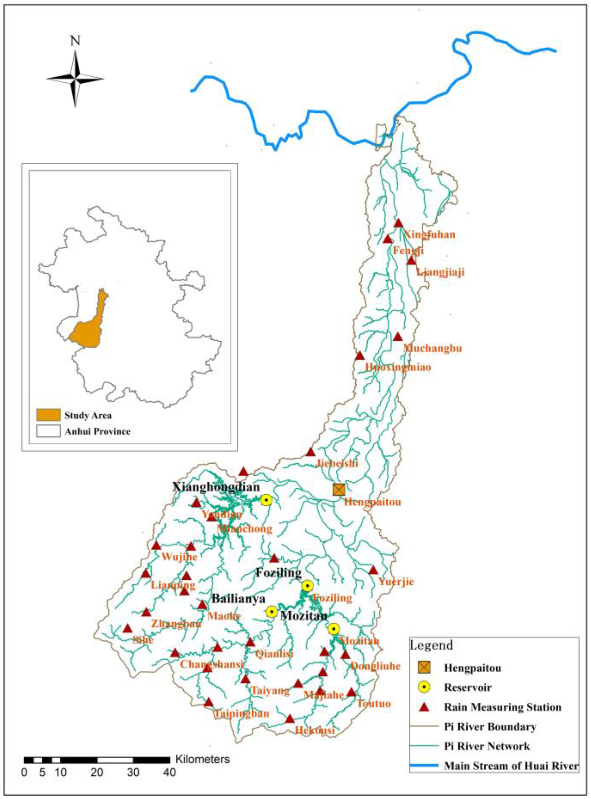
The Pi River Basin is a large tributary on the southern bank of the middle reaches of the Huai River. It originates from the northern foot of the Dabie Mountains and flows from south to north through counties and districts such as Yuexi, Huoshan, Jinzhai, Jin’an, Yu’an, Huoqiu, and Shouxian before joining the Huai River. The mountainous area covers 72% of the Pi River Basin, hills cover 17%, and plain depressions along the river cover the remaining 11% [23]. The terrain of the basin is a narrow and elongated strip, and the elevation goes down from south to north. According to the terrain and the confluence conditions, the area above the Fuziling and Xianghongdian Reservoirs can be defined as the upper reaches, with a mountainous catchment area of 3240 km2. The region from the above-mentioned two reservoirs to Hengpaitou is the middle reaches, with a catchment area of 1130 km2. The area from Hengpaitou to the river mouth is the lower reaches, with a basin area of 1630 km2, which consists of hilly and plain depressions [24].
The Pi River Basin is located between the Yangtze River and the Huai River on the northern foot of the Dabie Mountains. It falls in the North Subtropical Continental Monsoon Climate Zone, where cold and warm air masses frequently converge, and many cyclones occur. The abundant and concentrated precipitation is formed due to the combination of frequent landfall of southeast typhoons and the uplift of the terrain in the Dabie Mountains. The inter-annual and intra-annual distribution of precipitation in the basin is extremely uneven, with differences of more than three times between the annual precipitation of flood and drought years. Precipitation in the basin generally happens from June to August, accounting for 50% to 60% of the annual precipitation. The rainstorm centers in the basin mostly locate upstream of Fuziling and Xianghongdian Reservoirs. On 13 July 1969 and 10 July 1991, two extreme heavy rainstorms occurred in the basin, and the rainstorm centers were located in the Huangwei River, which is upstream of the Fuziling Reservoir, with the maximum 24 h precipitation exceeding 300 mm.
2.2. Data Sources
The rainfall data used in this study were provided by the Hydrology Bureau of Anhui Province. Hourly rainfall observed data from 37 rain gauge stations in Pi River Basin from 2003 to 2021 was selected for the study. The location map of the stations is shown in Figure 1.
3. Methodology
3.1. General Idea of This Study
This research is carried out following the technical route of data extraction, data processing, DTW rain pattern generation, training of four machine learning models, rain pattern identification, and results analysis. The technical flowchart is shown in Figure 2.
3.2. Generation of DTW Rainfall Pattern
Rainfall has the characteristics of persistence and intermittency. Due to the different duration of rainfall events, this study selected the wide industry-used DTW algorithm to classify the rainfall patterns of all events. The classification result is used as the benchmark for the verification of four machine-learning classification models.
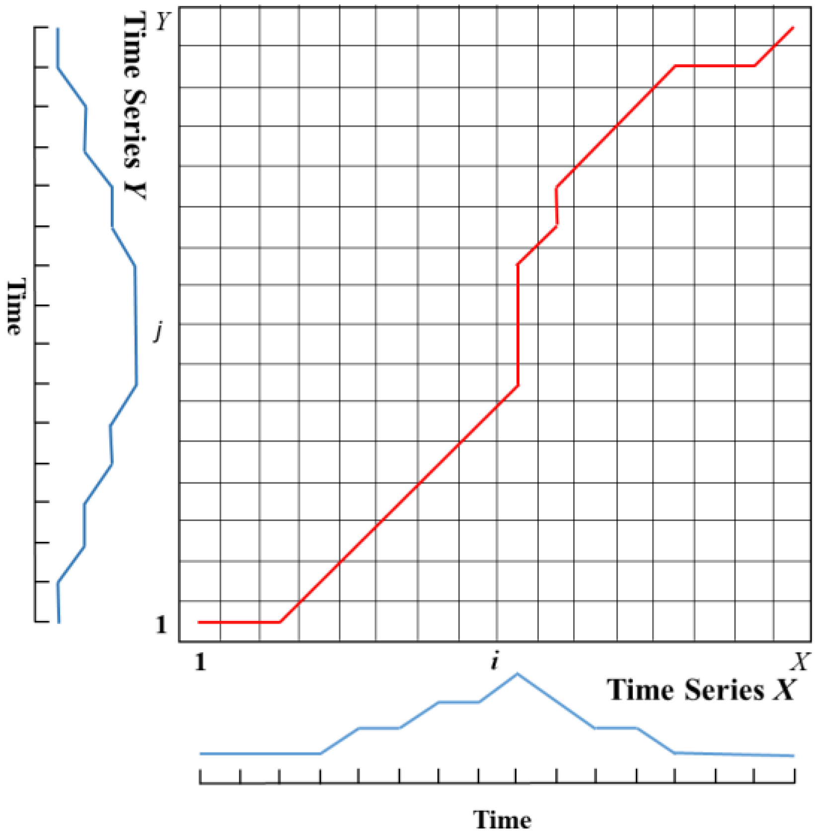
The DTW algorithm uses a time-warping function that satisfies specific conditions to describe the time correspondence between the test sequence and the reference sequence and computes the warping function that minimizes the accumulated distance between the two sequences during matching. An example of the algorithm is shown in Figure 3.
Assuming two continuous time series and , let be the distance function between corresponding points in the two sequences. Construct the distance matrix D between X and Y, and find the shortest path from the bottom-left corner to the top-right corner in D, which finds a suitable warping path φ to minimizes the accumulated distance between the two time series, as shown in Equations (1) and (2).
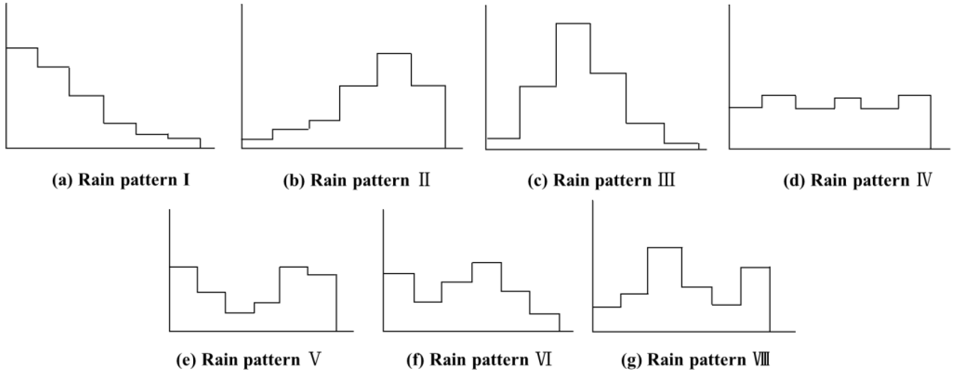
The seven rain patterns studied by Baogaomazowa (Soviet Union) and Cen Guoping (China) were taken as standard templates, among which pattern I, II, and III are single-peaked rain patterns, with their peaks located in the front, rear, and middle, named front- single-peak, rear-single-peak, and mid-single-peak, respectively. Pattern IV is a uniform rain pattern with little difference in rainfall distribution. Patterns V, VI, and VII are double-peaked rain patterns, with specific examples shown in Figure 4. According to the classification method of rain pattern in reference [11], each rain pattern can be divided into six stages, and based on the proportion of rainfall in each stage to the total rainfall, seven standard vector templates can be constructed [25], as shown in Formula (3).
Each rainfall is the event to be measured. By calculating the DTW values between the rainfall event and the standard rainfall template, the template pattern corresponding to the minimum DTW value is the rain pattern to which the rainfall event belongs.
3.3. Four Machine Learning Classification Methods Adopted in This Study
Based on the application results of previous scholars and industry [26,27,28,29], four models, namely DT, SVM, LSTM, and LightGBM, are widely used, and each has its own strengths in modeling structure, classification accuracy, and training efficiency. This study focuses on the comparison of the four classification algorithms, evaluating the models from the aspects of classification accuracy, training efficiency, classification effect, and stability in order to select the best model for building the best rainstorm pattern classification strategy.
3.3.1. Decision Tree
The Decision Tree (DT) is a method for approximating discrete function values. In 1984, Biman et al. [30] proposed the CART algorithm for DT, which uses a tree structure to evaluate. In 1986 and 1993, J Ross Quinlan introduced information gain and gain ratio, respectively, and proposed the ID3 and C4.5 algorithms.
Decision tree classification utilizes information theory’s information gain to search for the attribute field in the database with the maximum information content. It adopts a top-down divide-and-conquer approach to construct a classification rule in the form of a decision tree from a group of unordered and irregular instances [31].
Selecting the optimal splitting attribute is the key to decision tree classification, and information gain, gain ratio, and Gini index are generally used for splitting.
3.3.2. Long- and Short-Term Memory Neural Network
Long- and Short-Term Memory (LSTM) is an improved deep machine learning neural network based on RNN. In 1997, Hochreiter and Schimidhuber proposed the LSTM unit to effectively solve the problems of gradient explosion and gradient vanishing during RNN training, thereby truly utilizing long-distance sequence information [32].
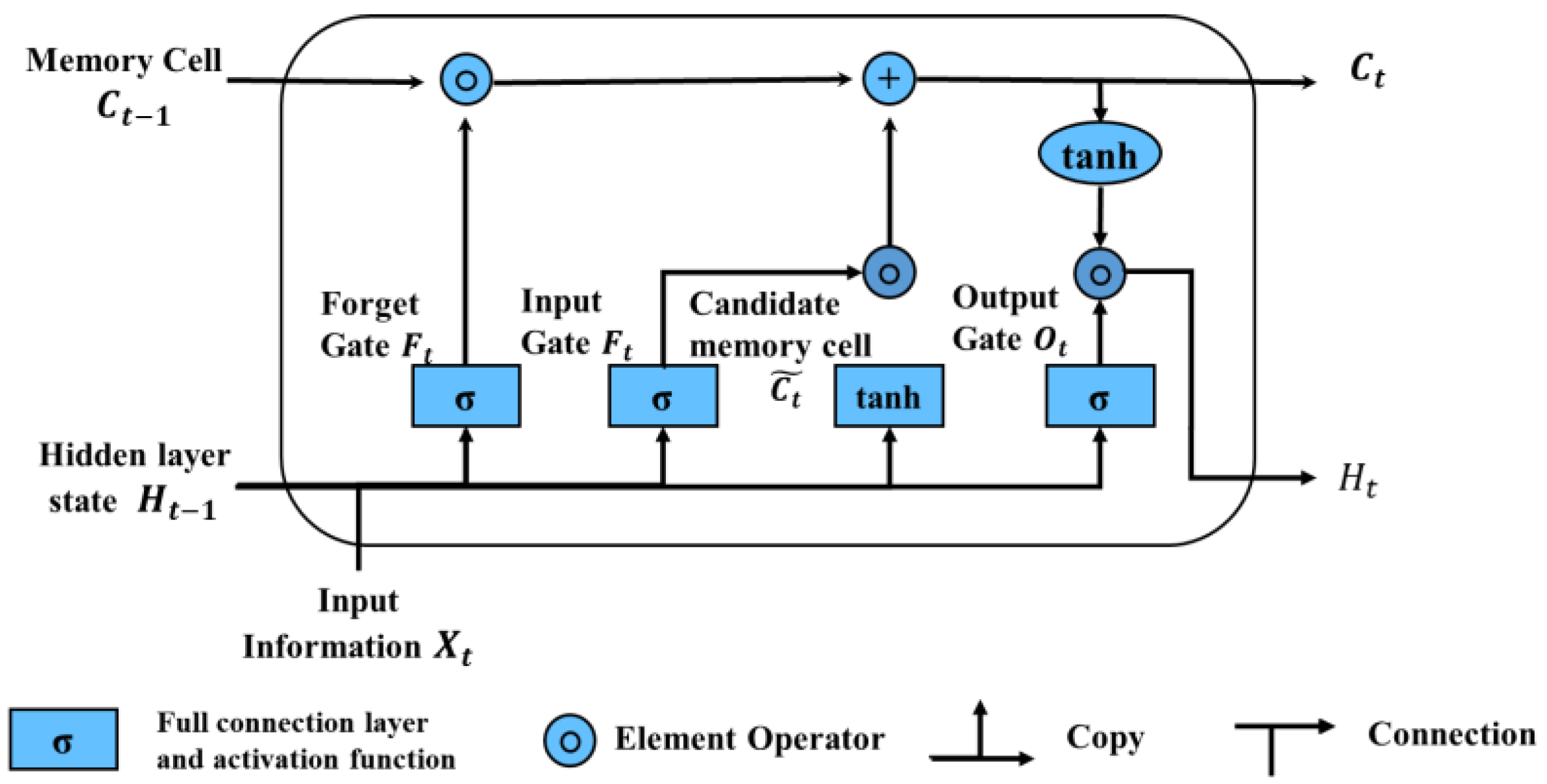
Like other neural networks, the LSTM model structure consists of an input layer, one or more hidden layers, and an output layer. The neurons in its hidden layers should not only receive information from the input layer but also receive information perceived by the neurons from the previous time step. At time t, the input to the memory cell includes the previous hidden layer state variable , the memory cell state variable , and the current input information . Then, the model sequentially obtains the hidden layer state variable and the memory cell state variable at time t through the forget gate , input gate , output gate , and these three control mechanisms. Finally, is passed to the output layer to generate the LSTM calculation result at time t, and together with , it is passed to the next time step for calculation. The overall structure of LSTM neural network is shown in Figure 5.
3.3.3. Support Vector Machine
Support Vector Machine (SVM) is a machine learning method proposed by Vapnik and Cortes in 1995 based on the principle of structural risk minimization in computational learning theory. It can improve the generalization ability of the learning machine and is suitable for binary classification problems and linearly inseparable problems.
The basic idea of SVM is to find a partition hyperplane in the sample space based on the training sample set , so that the sum of distances from different class samples to the hyperplane is maximized, i.e., (Figure 6).
Fitcsvm is a MATLAB function used to train or cross-validate a support vector machine (SVM) model for binary classification of low or medium-dimensional predictive variable data sets. It supports the use of kernel functions to map predictive variables, as well as sequential minimal optimization (SMO), iterative single data algorithm (ISDA), or L1 soft margin minimization (quadratic programming objective function minimization) methods.
The basic parameters include Box Constraint, Kernel Function, Kernel Scale, Polynomial Order, Standardize, etc. The Box Constraint is similar to the penalty factor (or regularization parameter). When the original data cannot exhibit good separability, the algorithm allows some misclassifications on the training set. The larger the value of the Box Constraint, the weaker the penalty strength, and the smaller the margin of the resulting classification hyperplane, the more support vectors, and the more complex the model. XOR problem and nonlinear mapping often exist in real tasks; the Kernel Function is used to calculate the inner product of feature space from the original sample space. The types of Kernel Functions include linear, polynomial, and Gaussian; the Kernel Scale parameter is used with the Gaussian kernel function in SVM. Polynomial Order is used with the Polynomial kernel function, indicating the degree of the polynomial kernel used. Standardize can standardize sample data to offset the interference caused by the distribution of feature data on classification.
3.3.4. Light Gradient Boosting Machine
Light Gradient Boosting Machine (LightGBM) is a scalable machine learning system launched by Microsoft Asia Research Institute in 2017. It is a distributed gradient-boosting framework based on the GBDT (Gradient-Boosting Decision Tree) algorithm. The main idea is to continuously construct new models in the direction of gradient descent of the previous model’s loss function so that the decision model can be continuously improved and then add up the conclusions of all trees as the final predicted output [33].
LightGBM is an advanced implementation of gradient-boosting decision trees. Its principle is similar to GBDT, which uses the negative gradient of the loss function as the residual approximation value of the current decision tree to fit a new decision tree. In other words, in each iteration, the original model remains unchanged, and a new function is added to the model to make the predicted value approach the true value.
The objective function of the training is shown in Formula (4)
where is the true label value, is the result of the K − 1th learning, and is the regularization term sum of the first K − 1 trees. The meaning of the objective function is to find a suitable tree that minimizes the value of the function.
Taylor formula is used to expand the objective function:
The second derivative Taylor expansion of the loss function is:
Let denote the first derivative of the loss function for the i-th sample, and denote the second derivative of the loss function for the i-th sample.
The simplified objective function is:
Traditional GBDT algorithm uses a pre-sorted algorithm to find the optimal split point when constructing decision trees, which requires traversing all data samples for each feature and calculating the information gain for all possible split points. LightGBM adopts an improved Histogram algorithm, which divides continuous floating-point feature values into k intervals and only needs to select the optimal split point among these k intervals, greatly improving the training speed and space utilization efficiency.
In addition, LightGBM reduces the amount of training data by using a leaf-wise strategy instead of a level-wise strategy when building decision trees and adds a maximum depth limit to ensure high efficiency while preventing overfitting. Gradient-based one-side sampling (GOSS) is used to retain instances with larger gradients while randomly sampling instances with smaller gradients to obtain accurate information gain estimates with a smaller amount of data. From the perspective of reducing features, exclusive feature bundling (EFB) is used to merge mutually exclusive features within a certain conflict ratio, achieving dimensionality reduction without losing information.
4. Construction of Rain Pattern Classification Model for Pi River Basin
4.1. Data Sources and Feature Selection
4.1.1. Data Sources
The data in this section was obtained from the extraction of rainfall events and the classification of rain patterns by using DTW. Based on a long series of rainfall data from the Pi River Basin spanning from 2003 to 2021, the rainfall data were divided into 11,808 events with a minimum rainfall duration of 6 h. Among them, there were a total of 5710 effective rainfall events (a rainfall event is defined as its cumulative rainfall greater than 2 mm).
The characteristics of duration and cumulative rainfall of each rainfall event were counted, and the similarity between rainfall events and standard rainfall templates was studied by using DTW to determine the pattern of rainfall. Table 1 shows the statistical results of seven patterns of rainfall in the Pi River Basin from 2003 to 2021 extracted by using the DTW method.
4.1.2. Feature Selection
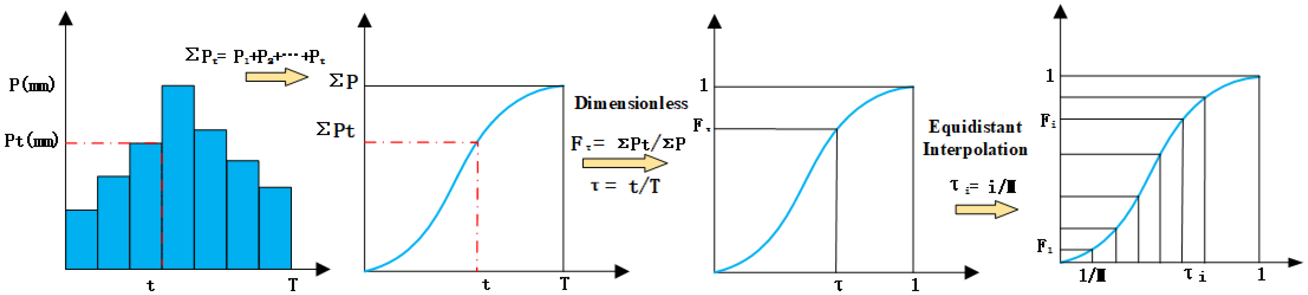
The rain pattern reflects the process of precipitation occurrence, development, and dissipation, which is numerically represented by the temporal distribution of accumulated rainfall over the precipitation duration. To eliminate the influence of precipitation characteristics so that the variation of precipitation intensity over time is the only factor affecting different rain patterns, the standardization of rainfall time series was carried out.
For each rainfall event, this study analyzed the total rainfall duration, total rainfall amount, cumulative rainfall duration, and cumulative rainfall amount, divided the cumulative rainfall amount by the total rainfall amount and used the quotient as the vertical axis, and divided the cumulative rainfall duration by the total duration and used the quotient as the horizontal axis to obtain the dimensionless accumulation rainfall mass curve of the rainfall process. We set the starting point of the dimensional-accumulation rainfall duration as 0, the endpoint as 1, and divided the x-axis span into 21 equal parts at intervals of 0.05 to obtain 21 corresponding cumulative rainfall percentages and complete the sample standardization. The first and 21st cumulative rainfall percentages of the standardized sample were 0 and 1, respectively. They did not contribute to the difference in classification results and were considered redundant features. Therefore, the representative 2nd to 20th cumulative rainfall percentage values were retained as independent variable features. The schematic diagram of the standardization process of rainfall event time series is shown in Figure 7.
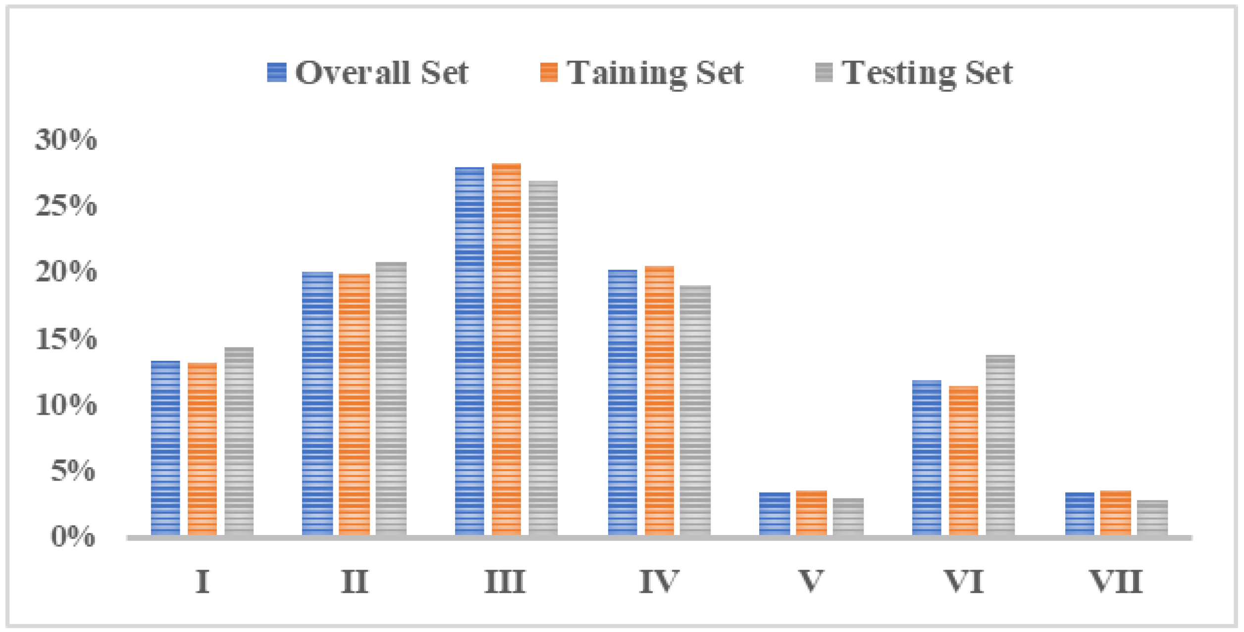
After sample standardization, a dataset including 5710 samples and 19 feature variables was formed. To facilitate model input, labels were set for the 19 independent variable features, namely T1, T2, …, and T19. The dependent variable label was based on the rainfall pattern classification results obtained by using DTW and divided into 1–7 categories. By analyzing the maximum rainfall intensity, rainfall peak position, total rainfall amount, etc., the training and validation datasets were specifically selected to make sure that the distribution of the validation set and training set was uniform and close to the overall rainfall pattern distribution characteristics. Eighty percent of the overall dataset was artificially selected as the training set and 20% as the validation set to perform multiclassification on the rainfall patterns in the Pi River Basin. The overall set, training set, and validation set proportion of each rainfall pattern in the Pi River Basin are demonstrated in Figure 8.
Considering that the number of samples may have a certain impact on the classification results, 500, 1000, 2500, and 5000 sample sets were designed. The training and validation set division criteria and model parameters (except for SVM, which uses automatic hyperparameter optimization) were the same as the overall set, and the number of iterations was adjusted accordingly. The distribution of the sample sets and the labeled classification are shown in Table 2.
4.2. Model Development and Numerical Test
4.2.1. Model Framework
The classification models developed in this article run on a 64-bit Windows 10 operating system. The development platform for LSTM and LightGBM is Python 3.6.8+JetBrains Pycharm, with the LSTM software framework being TensorFlow and LightGBM using the LGBMClassifier algorithm. The development platform for the Decision Tree is Jupyter Notebook, and the SVM development platform is Matlab 2022, using the Fitcsvm algorithm.
4.2.2. Model Parameters
The initial parameter values of the corresponding machine learning methods were set according to the algorithm characteristics and parameter adjustment experience of the four classification models. For the DT model, the feature selection criterion was based on entropy. The feature splitting point selection method was set to “best”. The maximum tree depth was set to 8, the minimum number of samples required for node splitting was set to 20, and the minimum number of samples required for leaf nodes was set to 10.
The LSTM model was constructed with 5 layers: 1 input layer, 3 hidden layers, and 1 output layer, with 32 neuron units per hidden layer. The input feature dimension was 19, and the output feature dimension was 7 classes. The optimizer was set to “adam”, with a learning rate of 0.1. The loss function was sparse categorical cross-entropy, which was a multi-class cross-entropy function. The batch size was set to 64, and the number of training epochs was set to 200.
As for the SVM model, the algorithm parameters were set to relatively simple. The Kernel Function was set to “Gaussian”, and the Loss function was set to “cross-entropy”. The optimized hyperparameters module was used to optimize the Box Constraint and Kernel Scale parameters to minimize the cross-validation loss, which was used as the optimization objective.
As for the LightGBM algorithm, six parameters were set: boosting type was “gbdt”; the number of trees to fit was set to 100; the learning rate was set to 0.1; maximum tree depth was set to 5; the maximum number of leaves per tree was 31; and the objective was for multi-class classification.
4.3. Model Evaluation
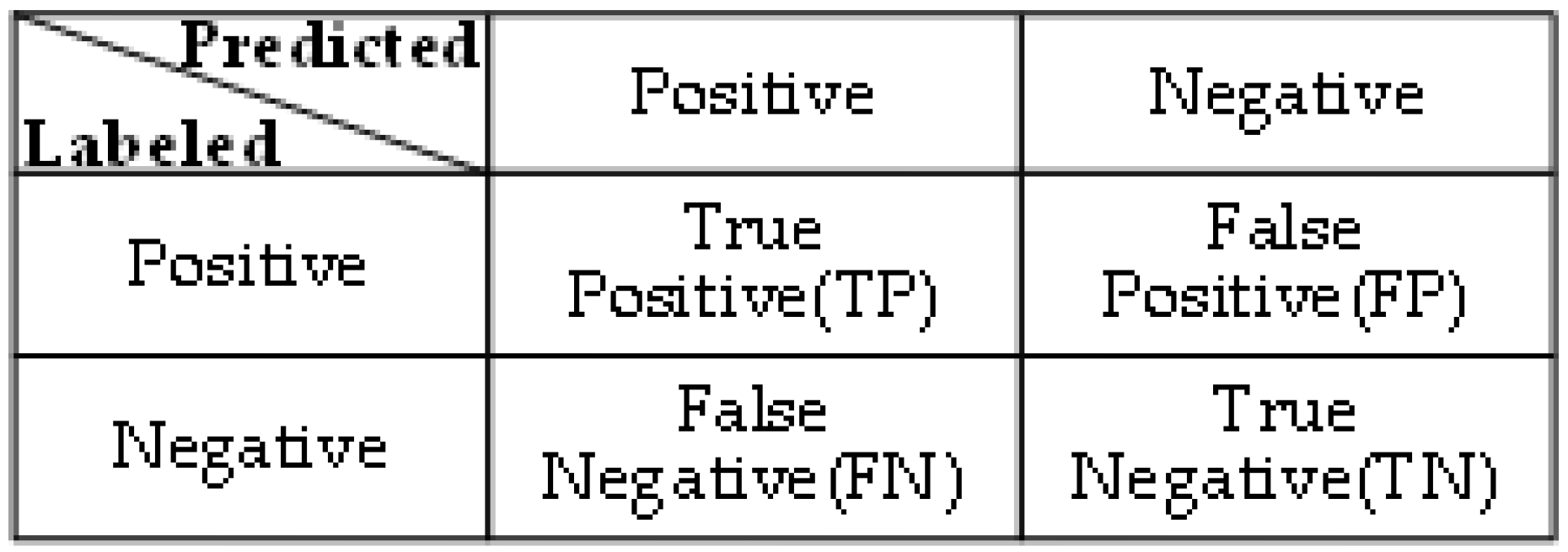
This article mainly uses the Confusion matrix and Loss function to evaluate the performances of four types of classification models. The confusion matrix is an analytical table used in machine learning to summarize the results of a classification model. Each column in the table represents a classification category, and each row represents the true type of data. The values on the diagonal represent the number of correctly classified samples. The larger and darker the values on the diagonal of the confusion matrix, the better the model’s classification performance. The metrics derived from the confusion matrix, such as accuracy, precision, recall, and F1 score, are essential evaluation metrics in machine learning. They are defined as follows (taking binary classification as an example, the confusion matrix is shown in Figure 9): TP represents the number of correctly identified targets, TN represents the number of other items correctly identified, FP represents the number of target items incorrectly identified, and FN represents the number of missed targets.
- (1)
- Accuracy (ACC)
Accuracy (ACC) represents the proportion of prediction accuracy among all prediction samples; the calculation method is shown in Equation (10):
- (2)
- Precision (P)
Precision (P) represents the proportion of predicted positive samples that are actually labeled positive, and the precision takes into account the proportion of positive samples that are predicted correctly; the calculation method is shown in Equation (11):
- (3)
- Recall (R)
Recall (R) refers to the proportion of predicted positive samples among actual labeled positive samples. Recall takes into account the proportion of recalled positive samples. The calculation method is shown in Equation (12):
- (4)
- F1 score
F1 score is the harmonic mean of precision and recall; the calculation method is shown in Equation (13):
Since the model used in this article was for multi-class classification, the macro-average rule was followed, which calculated precision, recall, and F1 score for each class separately and then took their mean; the calculation method is shown in Equations (14)–(16).
The log-loss function represents the confidence of the classification sample belonging to its corresponding class and is a loose measure of classification accuracy. It is expressed as follows.
The theoretical basis of log-loss is information entropy, so the larger the log-loss value, the more redundant noise there is, and the more it weakens the accuracy of the classification model.
5. Results and Discussion
5.1. Classification Results of DTW Rainfall Patterns
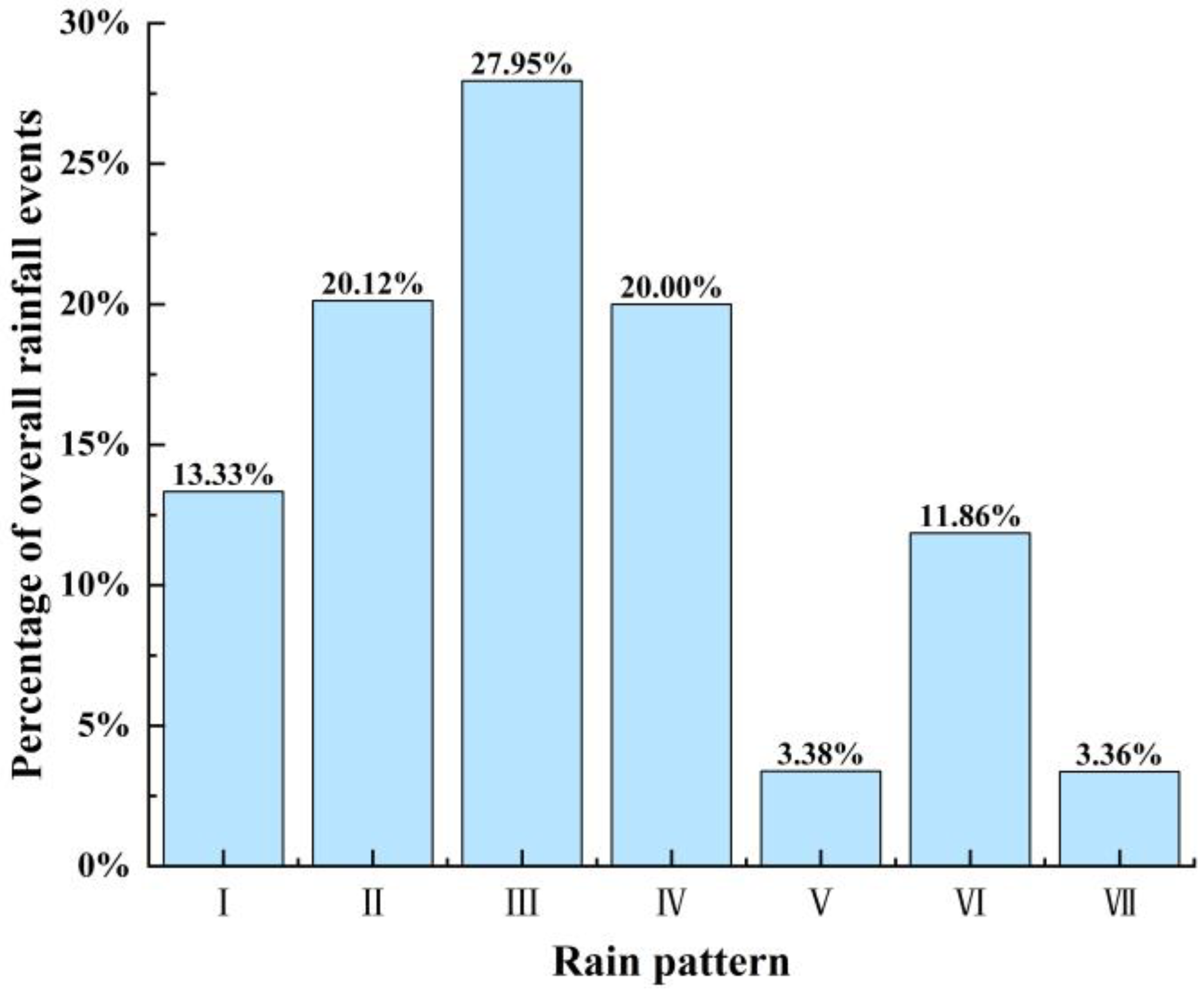
Percentages of different rain patterns in the Pi River Basin are shown in Figure 10. According to Table 1 and Figure 10, the rainfall patterns in the Pi River Basin are dominated by single-peak rainfall, mainly the pattern Ⅲ of mid-single-peak and the pattern Ⅱ of late-single-peak, which account for 27.95% and 20.12% of the total number of rainfall events, respectively. This is consistent with the research results in reference [34]. The rainfall duration is relatively long, which lasts for 22.2 h and 21.17 h, and the rainfall intensity is also high, at 0.99 mm/h and 0.96 mm/h, which indicates long-duration heavy rainfall. The second most common pattern is the pattern Ⅳ of uniform rainfall, which accounts for 20% of the total number of rainfall events, with a shorter average rainfall duration of 9.44 h and an average rainfall intensity of 0.95 mm/h. Double-peak rainfall is relatively rare in the basin, with the pattern Ⅵ of rainfall accounting for 11.86% of the total number of rainfall events and the patterns Ⅴ and Ⅶ of double-peak rainfall accounting for only 3.38% and 3.36% of the total number of rainfall events, respectively. However, the rainfall duration is long, and the rainfall intensity is high, and they all belong to long-duration heavy rainfall.
5.2. Comparison and Analysis of Four Machine Learning Classification Methods
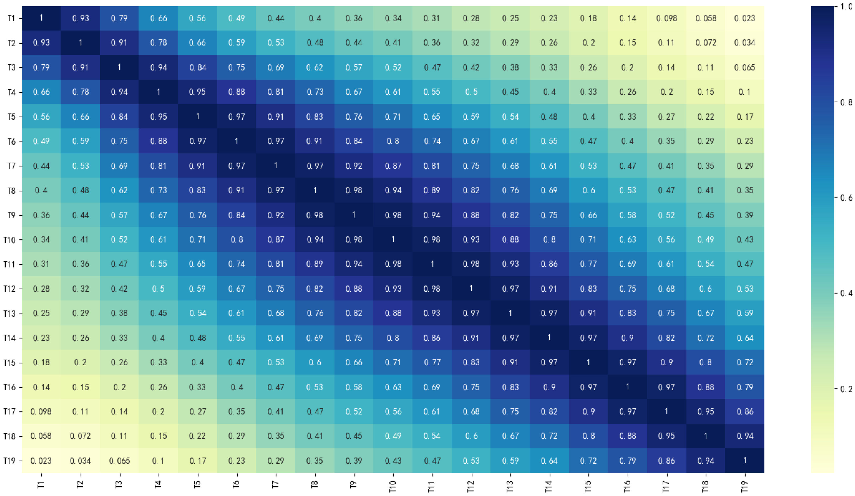
The accuracy evaluation of the four classification methods is shown in Table 3, and the loss convergence is shown in Figure 11, Figure 12 and Figure 13. Figure 14 shows the correlation coefficient of each factor index, which explains the unsatisfactory training effect of DT model; The confusion matrices of the classification results were visualized, and the results are shown in Figure 15.
As shown in Table 3, with DTW rainfall classification results as the reference benchmark, all four classification models achieved satisfactory classification accuracy. Among them, the LightGBM classification method had the highest accuracy, precision, recall, and F1 score values for the rainfall classification dataset, which were 98.95%, 99.25%, 97.96%, and 98.58%, respectively. The accuracy and F1 score were respectively improved by 0.18% and 0.27% compared to the LSTM classification method, by 1.32% and 1.26% compared to the SVM method, and by 3.6% and 5.4% compared to the DT method. Therefore, it can be seen that the LightGBM algorithm has improved all indicators of rainfall classification accuracy and is superior to the other three models.
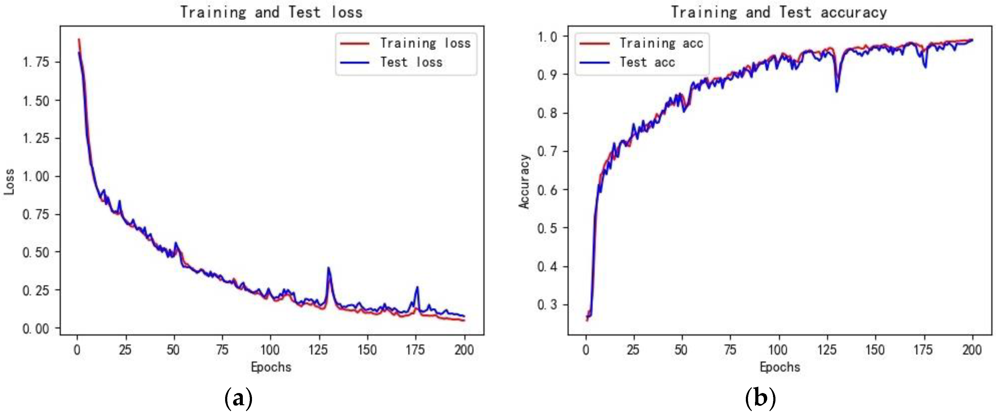
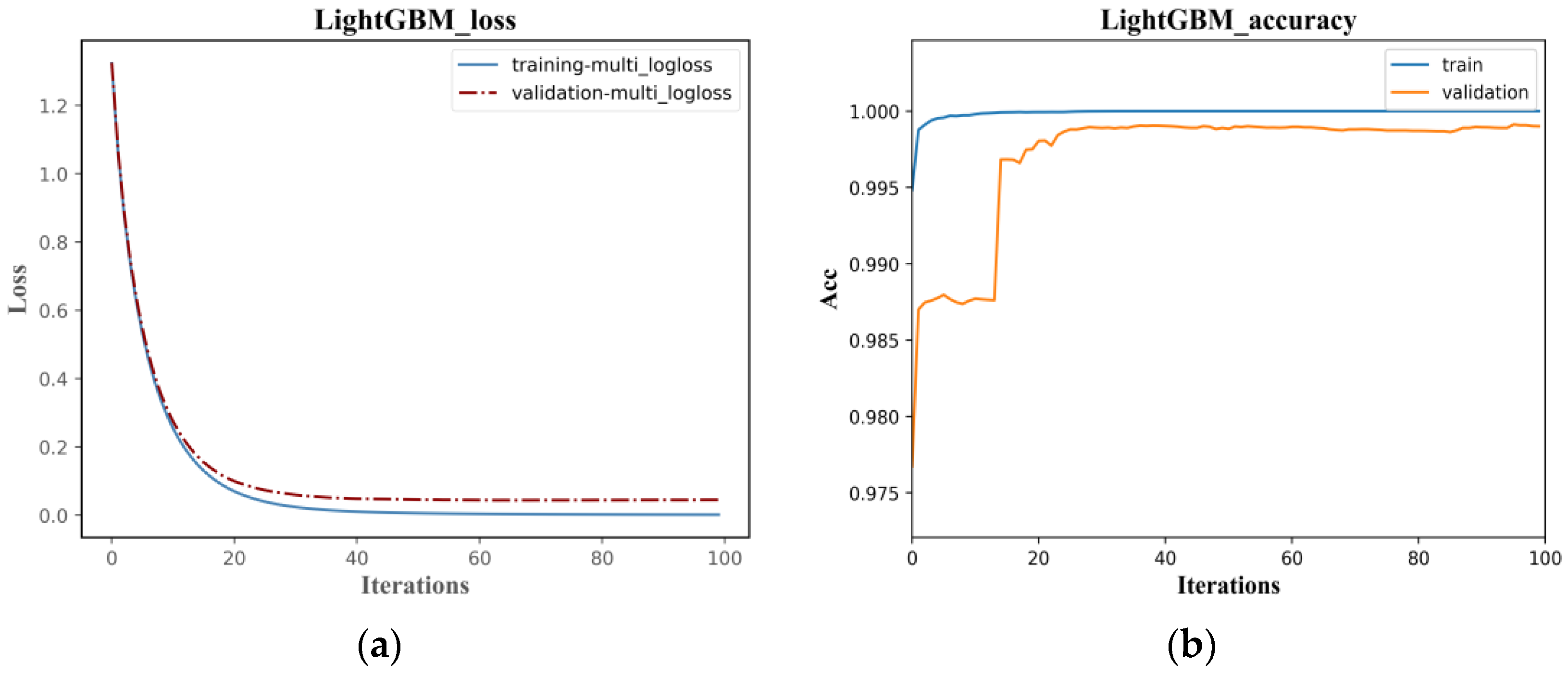
The classification accuracy of the LightGBM and LSTM models are similar, but the training efficiency of LightGBM is much higher than LSTM. As shown in Figure 12, the Loss function in the LightGBM classification model converges after 20 iterations, with the optimal cross-entropy losses of the training and validation sets being 0.0013 and 0.0444, respectively. The training set accuracy quickly converges in the early iterations, and the validation set accuracy tends to be stable after 20 iterations, with an overall shorter training time. Compared to the LightGBM model, the initial accuracy of the training and validation sets in the LSTM classification model is relatively low, with values of 0.2180 and 0.2680, respectively, and the Loss function values are high at 1.9296 and 1.8437, as shown in Figure 11. With the increase of the iteration times, the Loss function values gradually decrease, and the growth rate of accuracy increases. The accuracy reaches 0.9901 and 0.9871 after 200 iterations, with the Loss values decreasing to 0.0673 and 0.0809, respectively. The model tends to be stable and converges, but the training time is longer than that of LightGBM. Compared to the LightGBM model, the LSTM model has a relatively complex structure, and the characteristics of the recurrent network determine that the model cannot process data well in parallel. Additionally, the LSTM model has more parameters, resulting in lower training efficiency.
The classification accuracy of the SVM model is slightly lower than that of LightGBM and LSTM. The model uses quadratic programming to solve support vectors, involving the calculation of m-order matrices. Meanwhile, it utilizes a Bayesian-based hyperparameter optimization function to perform ten-fold cross-validation to minimize the best fit of the ‘Box Constraint’ and ‘Kernel Scale’ parameters. Due to a large amount of data, it requires a significant amount of machine memory and computation time, and it is not easy to find the optimal Kernel Function and classification parameters. It can be seen from Figure 13 that in the initial iterations, the cross-validation loss is relatively high, at 1.2774, but it quickly decreases and stabilizes at around 0.1284 after 30 iterations, eventually reaching convergence. Therefore, the classification efficiency of SVM is between that of LightGBM and LSTM.
Compared with the above three classification models, the classification performance of the DT model is the worst, but its training speed is fast, which is related to its simple model structure and fewer parameters. Previous studies have shown that DT performs well in small-scale, weakly autocorrelated datasets. The rainfall dataset used in this study is a time series with strong autocorrelation and cross-correlation, as shown in Figure 14, and the DT classification performance is normal, which verifies the relevant research conclusions.
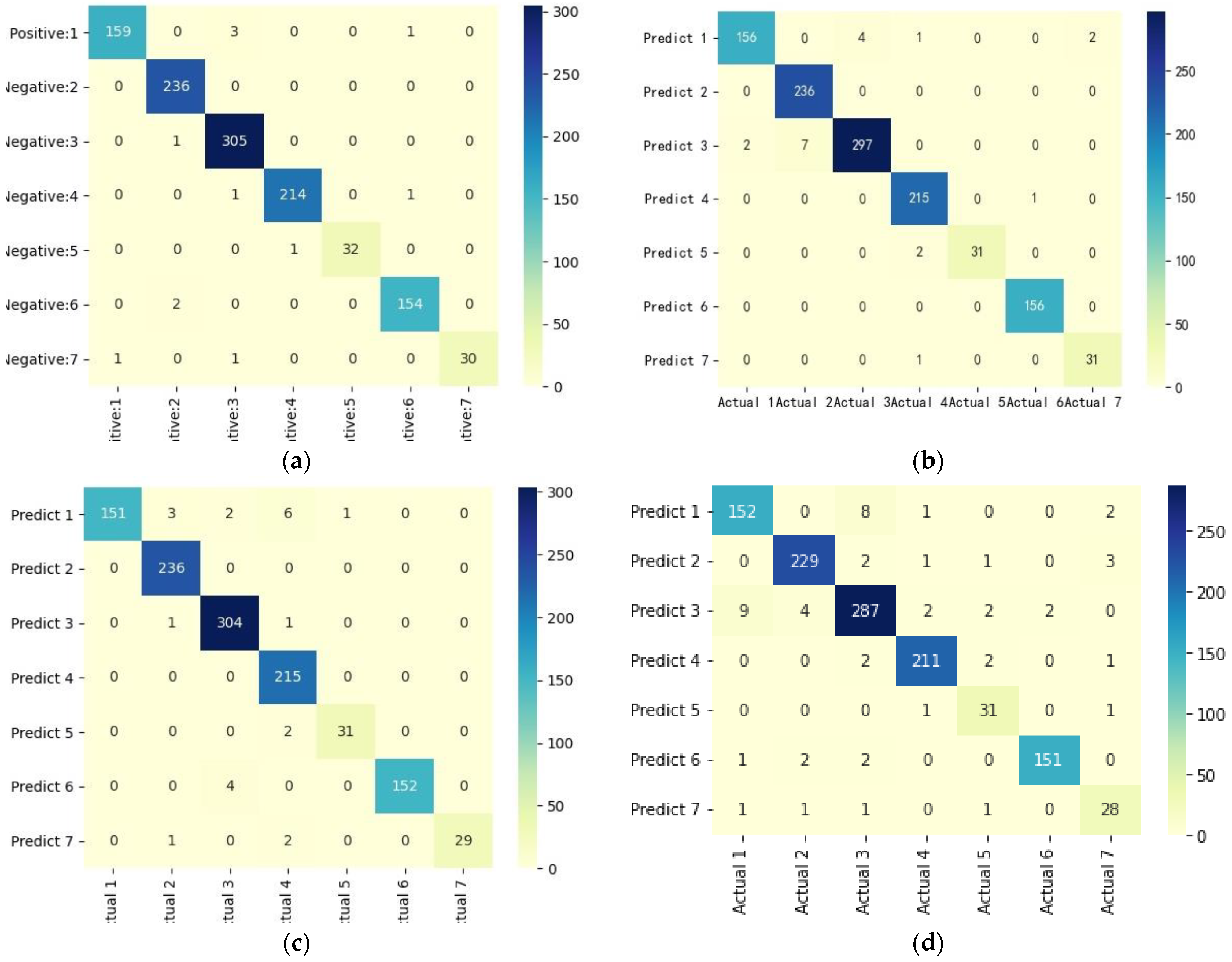
Figure 15 shows the confusion matrix of the four rainfall pattern classification models. Visually, all four models have achieved good classification performance, among which the LightGBM confusion matrix had the darkest diagonal color and the best classification effect, followed by the LSTM model and DT with the worst classification performance. All four models had a certain degree of misclassification, and the misclassified objects were not completely consistent. Table 4 shows the recall rate of each rain pattern based on different classification models.
In the rainfall dataset, the distribution of each rainfall pattern is uneven, with pattern III and pattern II rainfall samples accounting for 27.95% and 20.12% of the total, while pattern V and pattern VII account for only 3.38% and 3.36%, respectively. The average recall of pattern III and pattern II rainfall are 97.47% and 99.26%, respectively, while the recall of pattern V and pattern VII are lower, at only 94.70% and 92.19%. This indicates that when the sample distribution of each class is imbalanced, i.e., the number of samples of a certain class is much smaller than that of other classes, it will affect the classification accuracy of the model. In the classification of pattern V and pattern VII rainfall, the LightGBM model has a recall of 96.97% and 93.75%, with low classification errors, indicating that good classification results can be achieved even on imbalanced data.
Overall, in terms of model classification accuracy, training efficiency, classification performance, and stability, the LightGBM algorithm has the highest accuracy, fastest training efficiency, good classification performance, and stability on imbalanced data compared to the other three models. Therefore, it has strong applicability in the rainfall pattern classification of the Pi River Basin.
5.3. Analysis of Classification Results with Samples of Different Magnitudes
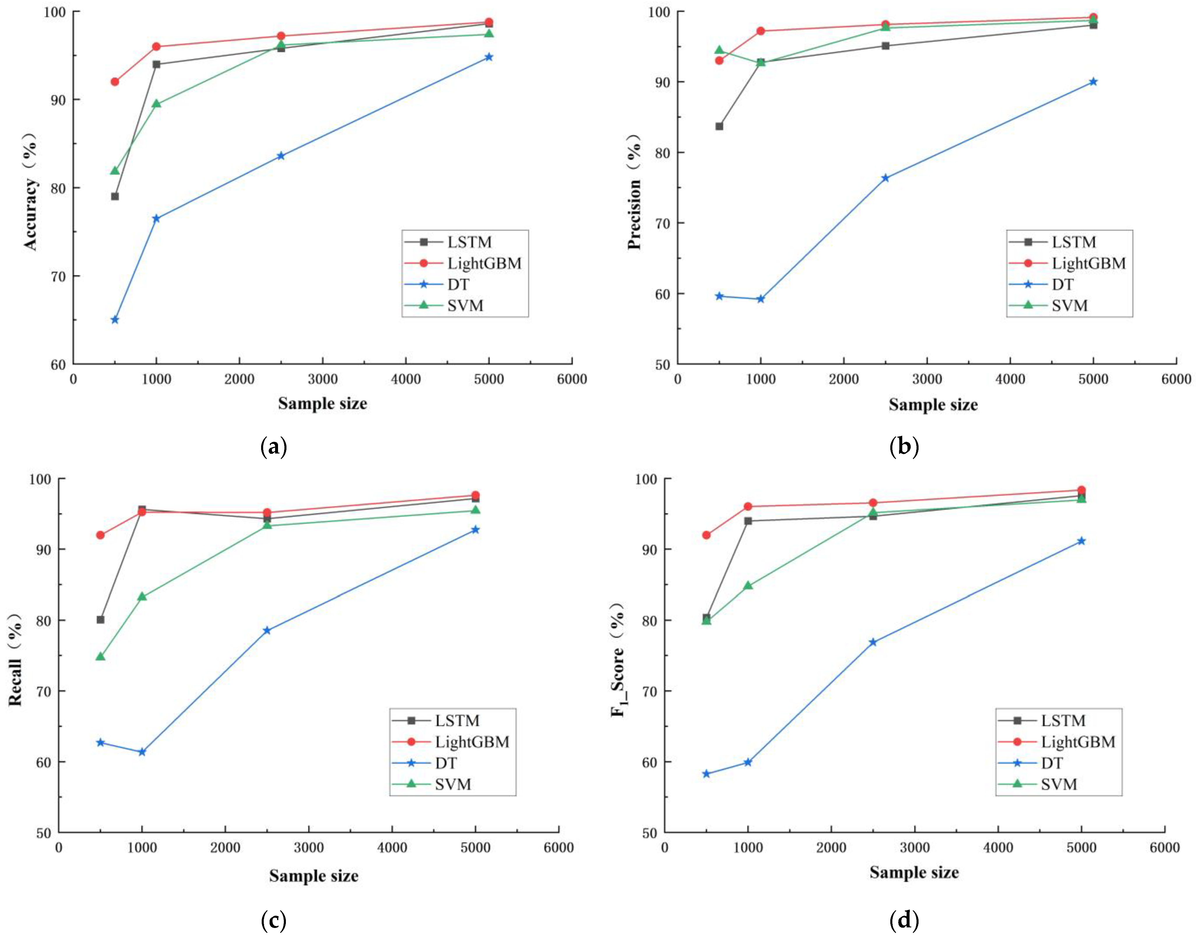
Under the conditions of 500, 1000, 2500, and 5000 rain pattern samples, four models were used to conduct classification simulation of rain pattern respectively, and the classification accuracy of four models were compiled and calculated for each rain pattern quantity, as illustrated in Table 5, according to the classification results, the distribution of four indexes including accuracy, precision, recall, and F1 score under different rain pattern samples are shown in Figure 16.
As can be seen from Table 5 and Figure 16, the accuracy, precision, recall, and F1 score of the four classification models generally increased as the sample size increased from 500 to 5000. Among them, the evaluation indicators of LightGBM and LSTM models did not increase significantly after the sample size increased to 1000, while those of DT and SVM models steadily increased with the increase in sample size. This indicates that the sample size has a significant impact on the accuracy of classification models.
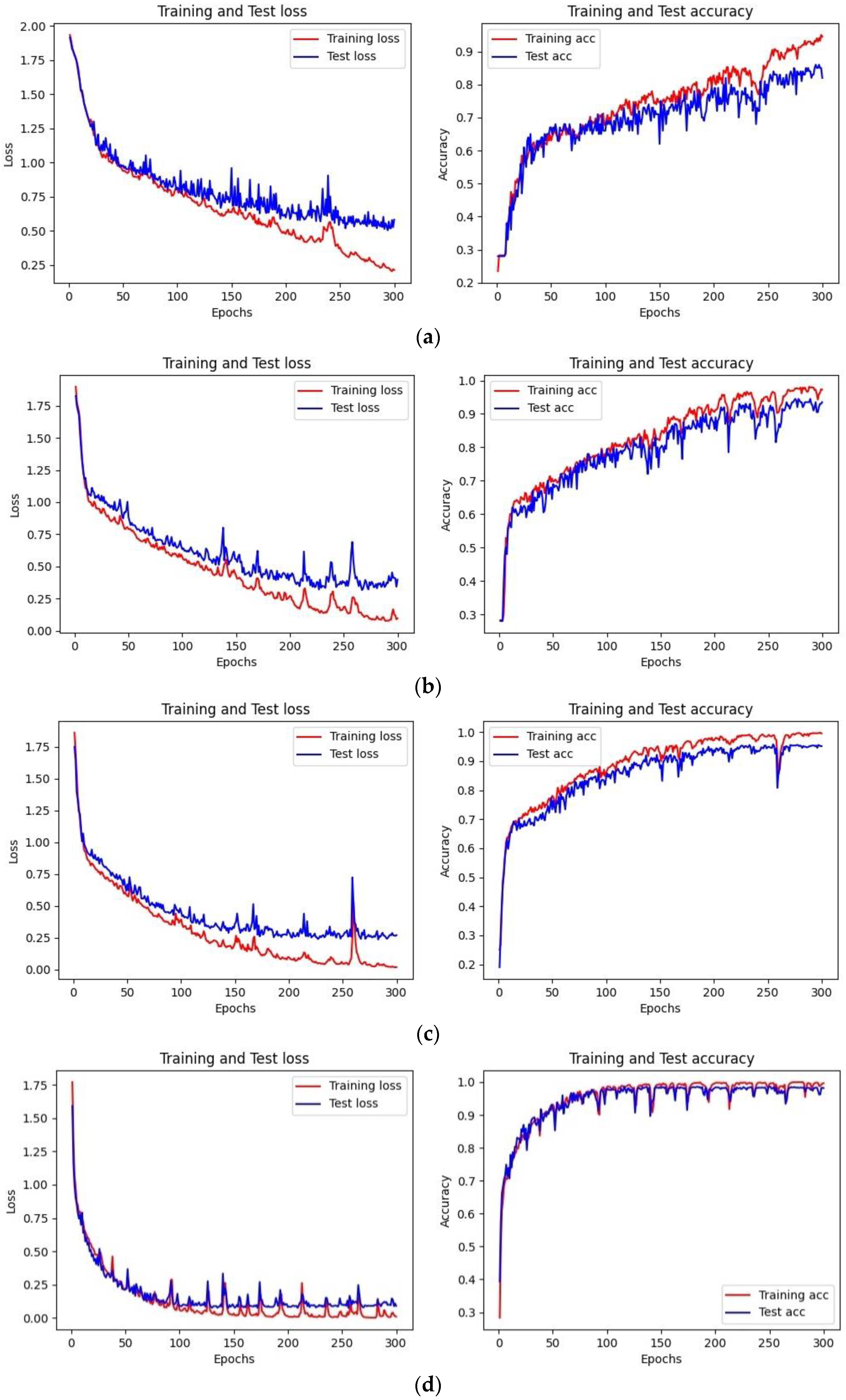
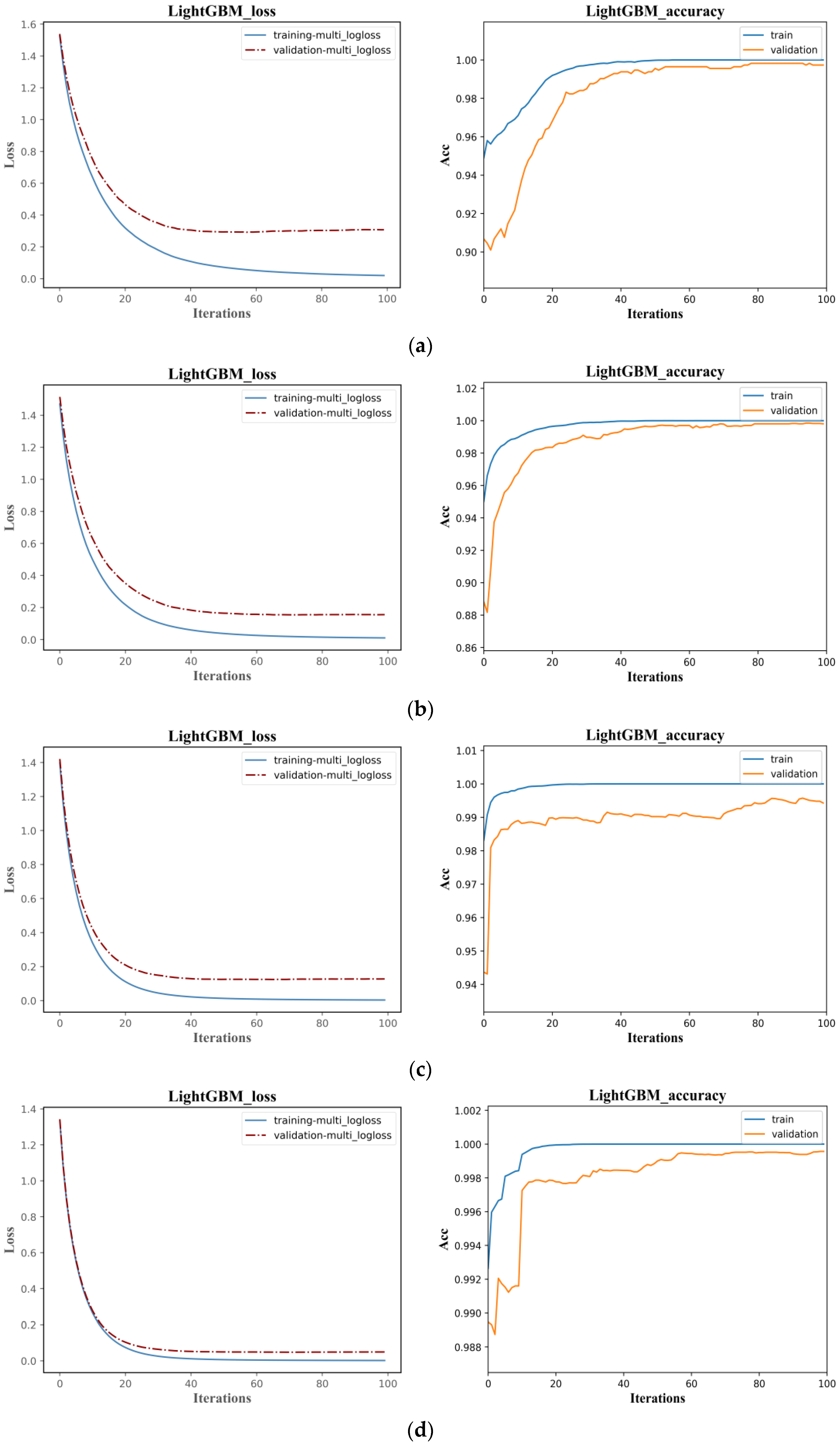
In order to further analyze the influence of different rain pattern samples on the model classification process, this study has compiled the changes in the loss function and accuracy of four models under different rain pattern samples. Taking LSTM and LightGBM models as examples, this study shows the changes in the loss function and accuracy of the models under the sizes of 500, 1000, 2500, and 5000 rain pattern samples, as shown in Figure 17 and Figure 18.
Overall speaking, as the number of samples increased, the Loss function values of the LSTM and LightGBM models on the training and validation sets steadily decreased, while the accuracy values steadily increased and eventually reached a stable convergence state. The initial and convergence Loss function values of the LSTM and LightGBM models were higher on small samples and lower on large samples. Taking the LSTM model as an example, when the sample size was 500, the initial value of the validation set Loss function was 1.9153, and the convergence speed was slow. After 300 iterations, it converged to 0.5182; when the sample sizes were 1000 and 2500, the initial values of the Loss function were 1.8786 and 1.7898, respectively, and the iteration speed accelerated. It reached stability at around 250 iterations and converged to 0.3681 and 0.2503, respectively. When the sample size was 5000, the initial value of the Loss function was 1.6438, and it converged quickly, stabilizing at around 100 iterations and converging to 0.1045. This shows that increasing the number of samples in machine learning classification helps to improve classification accuracy and training efficiency.
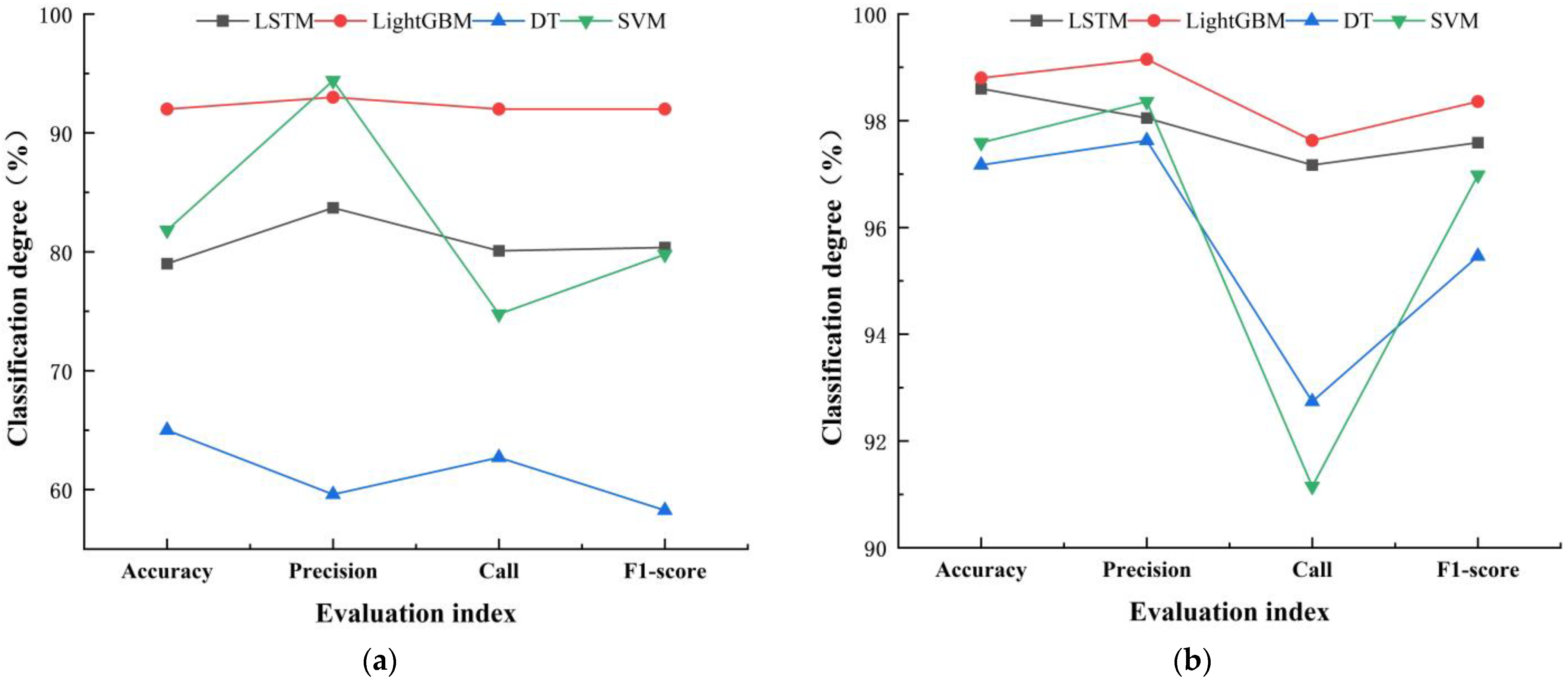
Previous studies have suggested that SVM models have certain advantages in dealing with small sample data [35,36,37]. In order to explore the performance of SVM models in handling classification problems with different numbers of rain pattern samples, this study compared a statistical analysis of the evaluation indicators of four models at rain pattern sample sizes of 500 and 5000, respectively, and presented the results in Figure 19.
When the sample size was 500, SVM had an accuracy rate of 81.82%, which was higher than LSTM and DT, and a precision rate of 94.40%, which was the highest among the four classification models. When the sample size increased to 5000, compared with the other three models, the accuracy and precision of SVM both decreased, and the recall tended to be the lowest among the four models. This result indicates that relative to large samples, SVM has certain advantages in handling small sample classification problems.
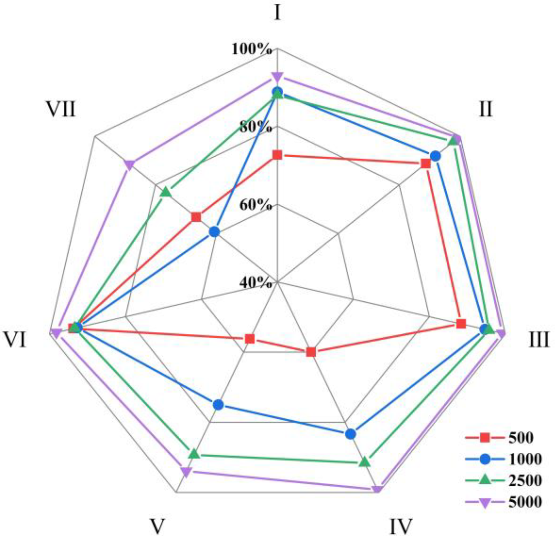
In order to investigate the impact of sample size on the accuracy of imbalanced sample classification, this study calculated the average recall of seven rain patterns of four models at sample sizes of 500, 1000, 2500, and 5000, as shown in Figure 20.
The average recall of each rain pattern for the four machine learning classification models at different sample sizes was calculated. The average recall for the pattern Ⅴ and pattern Ⅶ were lower than those of other rain patterns at different sample sizes, indicating that uneven distribution of rain patterns can affect classification performance. When the sample size was 500, the average recall of the pattern Ⅳ, which accounted for 20% of the total rainfall events, was only 60.00%, lower than that of the pattern Ⅵ, which accounted for 3.35% of the total rainfall events. This is because when the sample size is small, the rain-type distribution model is unstable, leading to unstable classification results.
5.4. Analysis of Characteristics Significance
LightGBM is a classification and regression technique that is not only suitable for nonlinear data modeling but also for analyzing the significance of variables to assist in characteristics selection and remove characteristics that are irrelevant or redundant to the target variable during the machine learning process, ultimately improving model accuracy and reducing runtime.
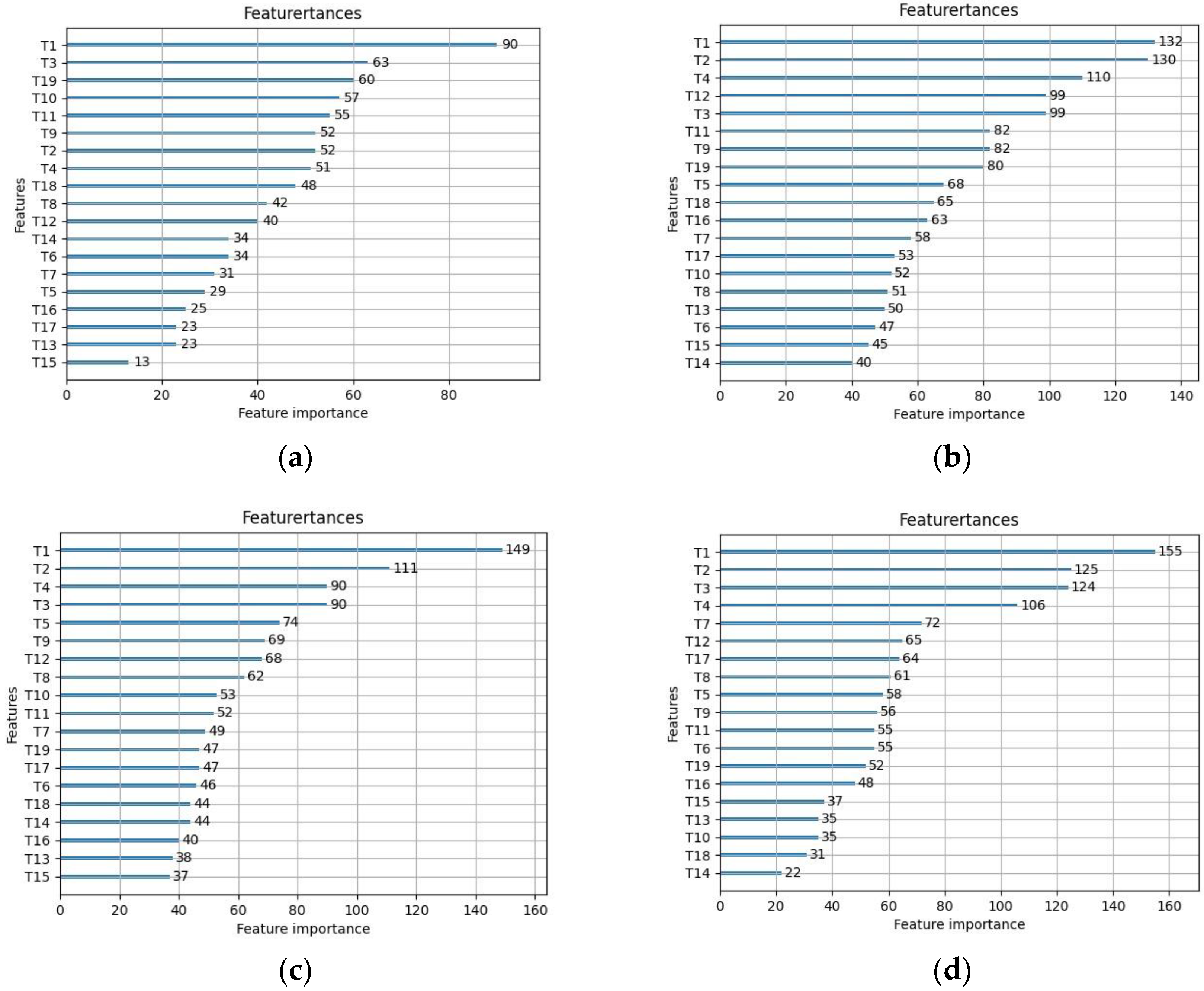
By using LightGBM to sort the significance of characteristics for different sample sizes, it can be observed from Figure 21 that the significance of each characteristic variable varies greatly with different sample sizes, mainly because the overall features are unstable in small samples, resulting in large classification result bias. The characteristic variable “T1” has the highest importance in all sample sizes and has a significant impact on the accuracy of classification results. As the sample size increases, the significance of characteristic variables “T2” and “T4” gradually increases and tends to stabilize. Characteristic variables “T14” and “T15” have poor importance and can be considered for removal to improve model classification accuracy.
6. Conclusions
Based on the analysis of precipitation events in the Pi River Basin using the DTW method, this article builds classification models based on DT, LSTM, SVM, and LightGBM algorithms. Through comparative analysis, it is found that the four machine learning models have strong generalization performance in precipitation event classification and achieve relatively good classification results. The specific conclusions are as follows:
(1) The overall classification effect of the LightGBM model is better than the other three models. Compared with LSTM and SVM models, LightGBM has simpler modeling, supports input of categorical features, is faster in speed, occupies less memory, and has higher learning accuracy and efficiency, about which the accuracy and F1 score were 98.95% and 98.58%, respectively, and the loss function and accuracy converged quickly after only 20 iterations. The imbalance in the number distribution of sample categories in the dataset will affect the classification accuracy of the model. LightGBM has significant advantages in solving classification problems with imbalanced category distribution. In practical applications, appropriate classification algorithms and data preprocessing methods can be selected based on the actual situation to achieve the classification goals more effectively.
(2) The sample size has a significant impact on the accuracy of the classification model. The reason is that the overall distribution is severely imbalanced in small samples, and increasing the sample size can improve the classification accuracy and training efficiency in machine learning classification. Compared with the other three models, the SVM model performs well in the small sample problem and has higher classification accuracy.
In summary, this article verifies the applicability of machine learning models in the field of rainfall pattern classification and expands the application scope of machine learning technology. Based on the current work, further research can be carried out, such as expanding one-dimensional rainfall time series to precipitation image sequence high-dimensional data to explore the classification of high-dimensional spatiotemporal sequences using machine learning methods; conducting random simulation on measured rainfall data, upgrading the sample size, adding noise data, and exploring the application effect of machine learning methods under conditions of large dataset randomness, mixed noise, and imbalanced categories.
Author Contributions
Conceptualization, G.K. and X.F.; methodology, X.F.; software, X.F.; validation, X.F., K.L. and R.L.; formal analysis, X.F.; investigation, X.F.; resources, R.L.; data curation, X.F. and K.L.; writing—original draft preparation, X.F.; writing—review and editing, X.F., G.K. and K.L.; visualization, X.F.; supervision, G.K., X.H. and L.D.; project administration, R.L. and L.D.; funding acquisition, R.L. All authors have read and agreed to the published version of the manuscript.
Funding
This research was funded by the National Natural Science Foundation of China: 42271095; IWHR Research and Development Support Program: JZ0199A032021; GHFUND A No. ghfund202302018283; National Key Research and Development Project: 2019YFC1510605; “Basic Research Type” Science and Technology Innovation Talent Program of Research Center of Flood & Drought Disaster Reduction of the Ministry of Water Resources: GY2205; Open Fund of Beijing Key Laboratory of Urban Water Cycle and Sponge City Technology: HYD2020OF02.
Institutional Review Board Statement
Not applicable.
Informed Consent Statement
Not applicable.
Data Availability Statement
Not applicable.
Acknowledgments
The authors also thank the anonymous reviewers for their helpful comments and suggestions.
Conflicts of Interest
The authors declare that they have no known competing financial interest or personal relationship that could have appeared to influence the work reported in this paper.
References
- Diederen, D.; Liu, Y. Dynamic Spatio Temporal Generation of Large Scale Synthetic Gridded Precipitation: With Improved Spatial Coherence of Extremes. Stoch. Environ. Res. Risk Assess. 2020, 34, 1369–1383. [Google Scholar] [CrossRef]
- Yuan, W.L.; Liu, M.Q.; Wan, F. Study on the Impact of Rainfall Pattern in Small Watersheds on Rainfall Warning Index of Flash Flood Event. Nat. Hazards 2019, 97, 665–682. [Google Scholar] [CrossRef]
- Kan, G.; Hong, Y.; Liang, K. Research on the Flood forecasting based on coupled machine learning model. China Rural. Water Hydropower 2018, 10, 165–169, 176. (In Chinese) [Google Scholar]
- Kan, G.; Liu, Z.; Li, Z.; Yao, C.; Zhou, S. Coupling Xin’anjiang runoff generation model with improved BP flow concentration model. Adv. Water Sci. 2012, 23, 21–28. (In Chinese) [Google Scholar]
- Mo, B. The Rain Water and Confluent Channel; Architectural Engineering Press: Beijing, China, 1959. [Google Scholar]
- Keifer, G.J.; Chu, H.H. Synthetic storm pattern for drainage design. J. Hydraul. Div. ASCE 1957, 83, 1332-1–1332-25. [Google Scholar] [CrossRef]
- Huff, F.A. Time distribution of rainfall in heavy storms. Water Resour. Res. 1967, 3, 1007–1010. [Google Scholar] [CrossRef]
- Pilgrim, D.H.; Cordery, I. Rainfall temporal patterns for design floods. J. Hydraul. Div. ASCE 1975, 101, 81–95. [Google Scholar] [CrossRef]
- Yen, B.C.; Chow, V.T. Design hyetographs for small drainage structures. J. Hydraul. Div. ASCE 1980, 106, 1055–1076. [Google Scholar] [CrossRef]
- Zhao, G. Time history allocation of design rainstorm type. Water Resour. Hydropower Eng. 1964, 1, 38–42. (In Chinese) [Google Scholar]
- Wang, M.; Tan, X.C. Study on urban rainstorm and rain pattern in Beijing. J. Hydrol. 1994, 3, 1–6. (In Chinese) [Google Scholar]
- Wu, Z.; Cen, G.; An, Z. Experimental study on slope confluence. J. Hydraul. Eng. 1995, 7, 84–89. (In Chinese) [Google Scholar]
- Cen, G.; Shen, J.; Fan, R. Study on rainstorm pattern of urban design. Adv. Water Sci. 1998, 9, 42–47. (In Chinese) [Google Scholar]
- Zhao, K.; Yan, H.; Wang, Y.; Tao, T. Influence of Rainfall Pattern and Intensity on Local Sensitivity of SWMM model parameters. Water Purif. Technol. 2018, 37, 95–101. (In Chinese) [Google Scholar]
- Zhang, X. Estimation of Hydrological Parameters and Identification of Influencing Factors of SWMM Model by Bayesian Statistics; Chongqing University: Chongqing, China, 2019. (In Chinese) [Google Scholar]
- Tu, X. Study on Mountain Flood Disaster Warning Model Based on Rain Pattern Clustering and Recognition; Zhengzhou University: Zhengzhou, China, 2021. (In Chinese) [Google Scholar]
- Yang, S.X. Research on Optimization of Rainfall Runoff Data-Driven Model Based on Deep Learning and Data Mining; Chongqing University: Chongqing, China, 2021. [Google Scholar]
- Gupta, U.; Jitkajornwanich, K.; Elmasri, R.; Fegaras, L. Adapting K-Means Clustering to Identify Spatial Patterns in Storms. In Proceedings of the 2016 IEEE International Conference on Big Data (Big Data), Washington, DC, USA, 5–8 December 2016. [Google Scholar]
- Gao, C.; Xu, Y.; Zhu, Q.; Bai, Z.; Liu, L. Stochastic generation of daily rainfall events: A single-site rainfall model with Copula-based joint simulation of rainfall characteristics and classification and simulation of rainfall patterns. J. Hydrol. 2018, 564, 41–58. [Google Scholar] [CrossRef]
- Yin, S.; Wang, Y.; Xie, Y.; Liu, A. Time-history classification of rainfall processes in China. Adv. Water Sci. 2014, 25, 617–624. (In Chinese) [Google Scholar]
- Xiao, K.L.; Zhao, G.L.; Wang, Y.; Hu, C.J. Spatial and temporal distribution of rainfall in flood season in Beijing city based on dynamic cluster analysis and fuzzy pattern recognition. J. Hydrol. 2019, 39, 74–77. (In Chinese) [Google Scholar]
- Hu, R.; Wang, S.; Wang, P. Study on short-duration rainstorm pattern based on cluster analysis. Water Resour. Power 2021, 39, 8–10. (In Chinese) [Google Scholar]
- Li, Y.; Yang, T.; Ma, J. Variation characteristics of precipitation concentration and concentration period during flood season in Pihe River Basin. Resour. Sci. 2012, 34, 418–423. (In Chinese) [Google Scholar]
- Zhang, Z.; Xue, C.; He, X.; Li, J.; Wang, F. Study on Joint flood control operation in Pihe River Basin, a tributary of Huaihe River. China Flood Drought Manag. 2020, 30, 13–18. (In Chinese) [Google Scholar]
- Li, Y.; Wang, Y.; Ma, Q.; Liu, T.; Si, L.; Yu, H. Study on the Characteristics of rainfall and rain Pattern Zoning in Hebei Province based on DTW and K-means algorithm. J. Geo-Inf. Sci. 2021, 23, 860–868. (In Chinese) [Google Scholar]
- Song, X.; Duan, Z.; Jiang, X. Comparison of Artificial Neural Networks and Support Vector Machine Classifiers for Land Cover Classification in Northern China Using a SPOT-5 HRG Image. Int. J. Remote Sens. 2012, 33, 3301–3320. [Google Scholar] [CrossRef]
- Pan, H.; Li, Z.; Tian, C.; Wang, L.; Fu, Y.; Qin, X.; Liu, F. The LightGBM-based classification algorithm for Chinese characters speech imagery BCI system. Cogn. Neurodyn. 2023, 17, 373–384. [Google Scholar] [CrossRef] [PubMed]
- Hina, T.; Mutahir, I.M.; Zafar, M.; Maqsooda, P.; Irfan, U. Gender classification from anthropometric measurement by boosting decision tree: A novel machine learning approach. J. Natl. Med. Assoc. 2023; in press, corrected proof. [Google Scholar]
- Nesrine, K.; Ameni, E.; Mohamed, K.; Hbaieb, T.S. New LSTM Deep Learning Algorithm for Driving Behavior Classification. Cybern. Syst. 2023, 54, 387–405. [Google Scholar]
- Breiman, L. Classification and Regression Trees; Wadsworth: Belmont, CA, USA, 1984. [Google Scholar]
- Han, J.W.; Micheline, K. Data Mining—Concepts and Techniques; Higher Education Press: Beijing, China, 2001. [Google Scholar]
- Hu, X. Research on Semantic Relation Classification Based on LSTM; Harbin Institute of Technology: Harbin, China, 2015. (In Chinese) [Google Scholar]
- Han, Q.; Zhang, X.; Shen, W. Lithology identification based on gradient lifting decision tree (GBDT) algorithm. Bull. Mineral. Petrol. Geochem. 2018, 37, 1173–1180. (In Chinese) [Google Scholar]
- Wang, S.; Wu, R.; Xie, W.; Lu, Y. Study on Mountain flood disaster risk Zoning based on FloodArea: A case study of Pihe River Basin. Clim. Chang. Res. 2016, 12, 432–441. [Google Scholar]
- Fan, X. Research and Application of Support Vector Machine Algorithm; Zhejiang University: Hangzhou, China, 2003. [Google Scholar]
- Ding, S.; Qi, B.; Tan, H. Review on Theory and Algorithm of Support Vector Machine. J. Univ. Electron. Sci. Technol. China 2011, 40, 2–10. [Google Scholar]
- Yang, J.; Qiao, P.; Li, Y.; Wang, N. A review of machine learning classification Problems and Algorithms. Stat. Decis. 2019, 35, 36–40. [Google Scholar]
Figure 1.
Location map of rain gauge stations in the Pi River Basin.

Figure 2.
Technical flowchart.

Figure 3.
Example of DTW algorithm.

Figure 4.
Rain template.

Figure 5.
Overall structure of LSTM neural network.

Figure 6.
Schematic diagram of support vector and interval.

Figure 7.
Standardization process of rainfall time series.

Figure 8.
Distribution of rain patterns for the seven rain patterns concerning the overall set, training set, and validation set in the Pi River basin.
Figure 8.
Distribution of rain patterns for the seven rain patterns concerning the overall set, training set, and validation set in the Pi River basin.

Figure 9.
Binary confusion matrix.

Figure 10.
Percentages of different rain patterns in the Pi River Basin.

Figure 11.
Classification effect of LSTM models on rainfall patterns: (a) Training and validation loss; (b) Training and validation accuracy.
Figure 11.
Classification effect of LSTM models on rainfall patterns: (a) Training and validation loss; (b) Training and validation accuracy.

Figure 12.
Classification effect of LightGBM models on rainfall patterns: (a) Training and validation loss; (b) Training and validation accuracy.
Figure 12.
Classification effect of LightGBM models on rainfall patterns: (a) Training and validation loss; (b) Training and validation accuracy.

Figure 13.
Classification effect of SVM models on rainfall patterns: (a) Training and validation loss; (b) Training and validation accuracy.
Figure 13.
Classification effect of SVM models on rainfall patterns: (a) Training and validation loss; (b) Training and validation accuracy.

Figure 14.
Correlation coefficients among various features of rain patterns.

Figure 15.
Confusion matrix of four classification algorithms: (a) LightGBM model; (b) LSTM model; (c) SVM model; (d) DT model.
Figure 15.
Confusion matrix of four classification algorithms: (a) LightGBM model; (b) LSTM model; (c) SVM model; (d) DT model.

Figure 16.
Classification accuracy of four models with different sample sizes: (a) Accuracy; (b) Precision; (c) Recall; (d) F1 score.
Figure 16.
Classification accuracy of four models with different sample sizes: (a) Accuracy; (b) Precision; (c) Recall; (d) F1 score.

Figure 17.
Loss function and accuracy of different sample sizes of LSTM models: (a) Sample size = 500; (b) Sample size = 1000; (c) Sample size = 2500; (d) Sample size = 5000.
Figure 17.
Loss function and accuracy of different sample sizes of LSTM models: (a) Sample size = 500; (b) Sample size = 1000; (c) Sample size = 2500; (d) Sample size = 5000.

Figure 18.
Loss function and accuracy of different sample sizes of LightGBM models: (a) Sample size = 500; (b) Sample size = 1000; (c) Sample size = 2500; (d) Sample size = 5000.
Figure 18.
Loss function and accuracy of different sample sizes of LightGBM models: (a) Sample size = 500; (b) Sample size = 1000; (c) Sample size = 2500; (d) Sample size = 5000.

Figure 19.
Classification accuracy of the SVM model under 500 and 5000 sample size: (a) Sample size = 500; (b) Sample size = 5000.
Figure 19.
Classification accuracy of the SVM model under 500 and 5000 sample size: (a) Sample size = 500; (b) Sample size = 5000.

Figure 20.
Classification recall rate of different samples of various rain patterns.

Figure 21.
Order of importance of the LightGBM model with different sample sizes: (a) Sample size = 500; (b) Sample size = 1000; (c) Sample size = 2500; (d) Sample size = 5000.
Figure 21.
Order of importance of the LightGBM model with different sample sizes: (a) Sample size = 500; (b) Sample size = 1000; (c) Sample size = 2500; (d) Sample size = 5000.


Table 1.
Statistical Table of Seven Rain Patterns in Pi River Basin from 2003 to 2021.
| Pattern | I | II | III | IV | V | VI | VII |
|---|---|---|---|---|---|---|---|
| Number of rainfall events | 761 | 1149 | 1596 | 1142 | 193 | 677 | 192 |
| Proportion/% | 13.33 | 20.12 | 27.95 | 20.00 | 3.38 | 11.86 | 3.36 |
| Average rainfall duration/h | 22.47 | 21.17 | 22.20 | 9.44 | 26.28 | 17.01 | 27.08 |
| Average rainfall/mm | 23.06 | 20.42 | 22.05 | 9.00 | 25.25 | 17.00 | 25.36 |
| Mean rainfall intensity/mm/h | 1.03 | 0.96 | 0.99 | 0.95 | 0.96 | 1.00 | 0.94 |
Table 2.
Distribution of rain events in training and validation set with different sample quantities.
Table 2.
Distribution of rain events in training and validation set with different sample quantities.
| Number of Sample Sets | Category | I | II | III | IV | V | VI | VII |
|---|---|---|---|---|---|---|---|---|
| 500 | Training | 53 | 80 | 112 | 80 | 14 | 47 | 13 |
| Validation | 13 | 20 | 28 | 20 | 3 | 12 | 3 | |
| 1000 | Training | 107 | 160 | 224 | 161 | 27 | 95 | 27 |
| Validation | 27 | 40 | 56 | 40 | 7 | 24 | 7 | |
| 2500 | Training | 267 | 400 | 559 | 402 | 68 | 237 | 67 |
| Validation | 71 | 103 | 134 | 95 | 14 | 68 | 14 | |
| 5000 | Training | 533 | 800 | 1118 | 805 | 135 | 474 | 135 |
| Validation | 143 | 207 | 268 | 189 | 29 | 137 | 28 |
Table 3.
Comparison of precision evaluation of four classification models.
| Name of Classification Models | Accuracy/% | Precision/% | Recall/% | F1-Score/% |
|---|---|---|---|---|
| DT | 95.35 | 92.21 | 94.28 | 93.18 |
| LSTM | 98.77 | 99.15 | 97.51 | 98.29 |
| LightGBM | 98.95 | 99.25 | 97.96 | 98.58 |
| SVM | 97.63 | 98.84 | 95.99 | 97.32 |
Table 4.
Recall rate of each rain pattern based on different classification models.
| Recall/% | I | II | III | IV | V | VI | VII |
|---|---|---|---|---|---|---|---|
| DT | 93.25 | 97.03 | 93.79 | 97.69 | 93.94 | 96.79 | 87.50 |
| LSTM | 95.71 | 100.00 | 97.06 | 99.54 | 93.94 | 100.00 | 96.88 |
| LightGBM | 97.55 | 100.00 | 99.67 | 99.07 | 96.97 | 98.72 | 93.75 |
| SVM | 92.64 | 100.00 | 99.35 | 99.54 | 93.94 | 97.44 | 90.63 |
| Average | 94.79 | 99.26 | 97.47 | 98.96 | 94.70 | 98.24 | 92.19 |
Table 5.
Comparative analysis of classification results of different rain pattern samples.
| Name of Classification Models | Number of Samples | Accuracy/% | Precision/% | Recall/% | F1 Score/% |
|---|---|---|---|---|---|
| LSTM | 500 | 79.00 | 83.70 | 80.08 | 80.36 |
| 1000 | 94.00 | 92.79 | 95.62 | 94.00 | |
| 2500 | 95.80 | 95.10 | 94.32 | 94.67 | |
| 5000 | 98.60 | 98.05 | 97.17 | 97.59 | |
| LightGBM | 500 | 92.00 | 93.00 | 92.00 | 92.00 |
| 1000 | 96.00 | 97.20 | 95.24 | 96.03 | |
| 2500 | 97.20 | 98.13 | 95.20 | 96.56 | |
| 5000 | 98.80 | 99.15 | 97.63 | 98.36 | |
| DT | 500 | 65.00 | 59.60 | 62.71 | 58.26 |
| 1000 | 76.50 | 59.21 | 61.36 | 59.91 | |
| 2500 | 83.60 | 76.36 | 78.55 | 76.89 | |
| 5000 | 94.80 | 90.00 | 92.74 | 91.15 | |
| SVM | 500 | 81.82 | 94.40 | 74.76 | 79.78 |
| 1000 | 89.45 | 92.62 | 83.22 | 84.76 | |
| 2500 | 96.19 | 97.63 | 93.31 | 95.17 | |
| 5000 | 97.40 | 98.73 | 95.46 | 96.98 |
Disclaimer/Publisher’s Note: The statements, opinions and data contained in all publications are solely those of the individual author(s) and contributor(s) and not of MDPI and/or the editor(s). MDPI and/or the editor(s) disclaim responsibility for any injury to people or property resulting from any ideas, methods, instructions or products referred to in the content. |
© 2023 by the authors. Licensee MDPI, Basel, Switzerland. This article is an open access article distributed under the terms and conditions of the Creative Commons Attribution (CC BY) license (https://creativecommons.org/licenses/by/4.0/).
Share and Cite
MDPI and ACS Style
Fu, X.; Kan, G.; Liu, R.; Liang, K.; He, X.; Ding, L. Research on Rain Pattern Classification Based on Machine Learning: A Case Study in Pi River Basin. Water 2023, 15, 1570. https://doi.org/10.3390/w15081570
AMA Style
Fu X, Kan G, Liu R, Liang K, He X, Ding L. Research on Rain Pattern Classification Based on Machine Learning: A Case Study in Pi River Basin. Water. 2023; 15(8):1570. https://doi.org/10.3390/w15081570
Chicago/Turabian StyleFu, Xiaodi, Guangyuan Kan, Ronghua Liu, Ke Liang, Xiaoyan He, and Liuqian Ding. 2023. "Research on Rain Pattern Classification Based on Machine Learning: A Case Study in Pi River Basin" Water 15, no. 8: 1570. https://doi.org/10.3390/w15081570
Note that from the first issue of 2016, this journal uses article numbers instead of page numbers. See further details here.