
A Robust Regime Shift Change Detection Algorithm for Water-Flow Dynamics


1
Department of Geomatics Engineering, University of Calgary, 2500 University Drive NW, Calgary, AB T2N 1N4, Canada
2
Resource Stewardship Division, Alberta Environment and Parks, 3535 Research Road NW, University Research Park, Calgary, AB T2L 2K8, Canada
3
Department of Civil Engineering, University of Calgary, 2500 University Drive NW, Calgary, AB T2N 1N4, Canada
*
Author to whom correspondence should be addressed.
Water 2023, 15(8), 1571; https://doi.org/10.3390/w15081571
Submission received: 20 March 2023
/
Revised: 6 April 2023
/
Accepted: 13 April 2023
/
Published: 17 April 2023
(This article belongs to the Special Issue River Flow Monitoring: Needs, Advances and Challenges)
Abstract
:Stream and river monitoring have an influential role in agriculture, the fishing industry, land surveillance, the oil and gas industry, etc. Recognizing sudden changes in the behavior of streamflow could also provide tremendous insight for decision-making and administration purposes. The primary purpose of this study is to offer a new robust Regime Shift Change Detection (RSCD) algorithm which can identify periods and regime changes without any assumptions regarding the length of these periods. A regime shift algorithm using two different refined method approaches is proposed in this article. The RSCD with Relative Difference (RSCD-RD) and RSCD with Growth Rate (RSCD-GR) are the two main specializations of this regime shift algorithm. We compared these two specializations on train and test datasets and commented on the advantages and each specialization. RSCD-GR and RSCD-RD were equally effective in detecting regime changes when thresholds were pinpointed for each station and season. However, RSCD-RD outperformed RSCD-GR when general thresholds were used for cold and warm months. A strength of RSCD-GR is the ability to investigate newly observed data separately, while RSCD-RD may require re-investigation of historical data in some cases. A regime change was detected in the monthly streamflow data of the Athabasca River at Athabasca (07BE001) in May 2007, while no such change was observed in the monthly streamflow data of the Athabasca River below Fort McMurray (07DA001). The discrepancy could be attributed to factors such as the clarity of the river water from Saskatchewan or the utilization of industrial water. Additional investigation might be required to determine the underlying causes.
1. Introduction
Studying streamflow variation is an important topic due to the significance of management and monitoring of water resources for maintaining life and mitigating extreme seasonal discharge variation [1,2]. Human endeavors such as withdrawals, land cover transformations, and building reservoirs can modify steady discharge regimes and induce changes in the volume, timeframe, and period of flood occurrences [3,4]. Mountain watersheds play a crucial role in supplying water resources in semiarid and dry regions [5]. For watersheds dominated by snow, meltwater is the most considerable contributor to streamflow, and streamflow is vastly influenced by shifts in snowfall, snow-covered areas, and meltwaters [6,7]. Studying and identifying regime shifts resulting from temperature variation, meltwaters, precipitations, etc., is vital for overseeing water resources and managing climate change-associated hazards [7,8].
Online (real-time) and offline are the two primary classes of change detection techniques. In online change detection procedures, a given number of data points are investigated ahead of the candidate change point [9]. The main purpose of such methods is to pinpoint changes in comparative real-time with negligible delays [10]. On the other hand, offline change detection presumes that all data for a time series is known, and the main objective is to detect when the aspects of the time series change. The entire time series is processed at once using these online algorithms [9].
Rodionov categorized the regime shifts detection methods into four families of algorithms [11]. One of the most common regime shift algorithm families is those that include “Shifts in the Mean”, such as the Mann–Kendall test [12], the Pettitt test [13], Bayesian analysis [14], etc. Another family of regime shift algorithms is “Shifts in the Variance”, including the Downton–Katz test [15] and the Rodionov method [11]. The next family of regime shift detection, according to Rodionov, is “Shifts in the Frequency Structure”. The Nikiforov method [16] is an example of such a method. Finally, “Shifts in the System” are the last family of regime shift detection. As an example, the Vector auto-regressive method [17] and Principal component analysis (PCA) [18] are two methods from this family of regime shift detection.
There has been a number of studies dedicated to identifying regime shift detection of streamflow. Zhang et al. [4] proposed a method for analyzing regime change detection in the Yellow River basin in China between 1919 and 2011. The authors recommended comparing trends in four distinct annual stages: 1919–1933, 1934–1969, 1970–1986, and 1987–2011, and examining changes between each group. To investigate the regime shift between the stages, the authors employed the Breaks For Additive Seasonal and Trend (BFAST) method in conjunction with the Mann–Kendall (MK) test. However, the use of the MK test for detecting regime shifts has limitations because it requires dividing the period of interest into multiple stages [11]. Wang et al. [19] applied Rodionov’s Sequential T-test Analysis of Regime Shifts (STARS) to identify regime shifts in sediment and runoff loads for China’s Yellow River basin region. According to Rodionov [11], this algorithm is a “Shifts in the Mean” algorithm. While it can automatically pinpoint several change points and regime shifts in online mode (real-time), it mandates some examination when selecting the cutoff length and the confidence interval [11]. Khan et al. [20] incorporated the Mann–Kendall trend test [21] and change point investigation [22] for six different watersheds within the state of Illinois, USA, from the 1930s to the 2010s. As stated by Rodionov [11], although the Mann–Kendall test is very convenient to employ and it has a strong theoretical background, the data needs to not be influenced by a trend, and only a single change-point can be detected using the traditional version of this method.
Many regime shift algorithms suffer from a significant limitation in that they heavily rely on pre-existing assumptions and prior knowledge of the system being investigated. This can lead to inaccuracies and biases if the assumptions are inadequate or incorrect [11,23,24]. In addition, these algorithms may not be capable of detecting slow or gradual changes that occur over longer periods of time and instead can only identify sudden or rapid shifts. Furthermore, the accuracy of regime shift algorithms is highly dependent on the quality and quantity of available data, which can be limited in some cases [11,23,24].
Athabasca River Basin (ARB) has been one of the main contributors to the economy of Alberta province since the rise of the oil and gas industry in 1967. In addition to the oil industry, agriculture, forestry, mining, and tourism are other primary activities of this region [25]. The majority (approximately 82% of its land area) of the ARB is covered by boreal forest [26]. As a consequence of urban expansion and industrial commodity production, including agricultural expansion, forest degradation, mining of coal and oil, etc., the ARB has transformed abruptly over recent decades. Apart from these man-made activities, natural hazards such as wildfire also altered the landscape of the basin [25,26].
The objective of this research was to develop a regime shift change detection algorithm capable of operating in real-time or offline mode. The proposed algorithm requires only the mean and standard deviation of a baseline period, a threshold for pinpointing the period, and the time series itself. Our intention was to minimize requirements and provide efficient algorithms that can be easily implemented in real-time or offline mode. Since the accuracy and amount of available data significantly influence regime shift detection, we also employed Random Forest Regression and Seasonal Autoregressive Integrated Moving Average (SARIMA) models to mitigate the effects of data on our analysis and threshold identification. The paper is structured as follows: Section 2 details the study region, data sets, the Regime Shift Change Detection (RSCD) algorithm, and the threshold selection process. The results of the RSCD algorithm and exploratory analysis are presented in Section 3, followed by a discussion of the findings in Section 4. Finally, the paper concludes in Section 5.
2. Materials and Methods
2.1. Study Region
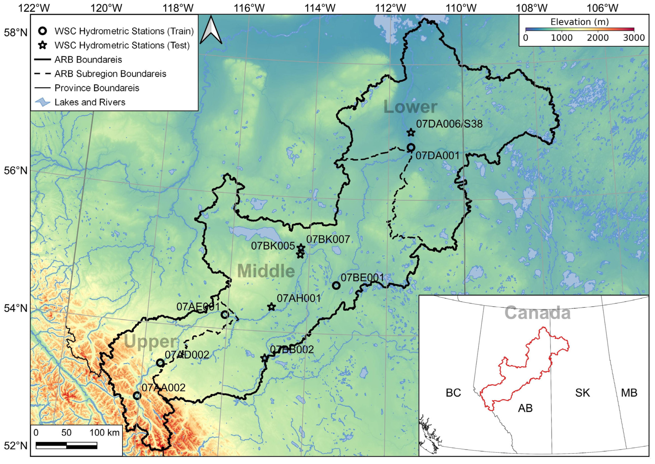
The Athabasca River Basin (ARB) is close to 160,000 km2, which is just under a quarter of Alberta’s province [27] and comprises numerous named/unnamed rivers and lakes. Both cold and warm seasons are available in this region. During cold months, a substantial portion of precipitation is in the form of snow, while during the warm months, meltwater and rainfall merge and contribute to river streamflow. Water from sub-basins likewise amalgamates with the main river as the river flows in the direction of Lake Athabasca [26,28]. The ARB region is shown in Figure 1, whose background gradient color was generated utilizing Shuttle Radar Topography Mission (SRTM) data sampled at 30 m. The ARB region includes three main subregions, namely, lower, middle, and upper [29].
2.2. Streamflow Data
The streamflow data used in this study were acquired from the Water Survey of Canada (WSC) (https://wateroffice.ec.gc.ca, accessed on 1 July 2022). The WSC gathers concurrent hydrometric data (streamflow and water level) at hydrometric gauging stations across Canada. In order to eliminate small gaps in the data for station 07DA006/S38 in the WSC dataset, the data from the Regional Aquatics Monitoring Program (RAMP) (http://www.ramp-alberta.org, accessed on 1 July 2022) were fused. Hydrometric stations shown in Table 1 were selected based on the period of records considering the availability of continuous data and extended periods of gaps in monitoring. Five of these stations (i.e., 07AA002, 07AD002, 07AE001, 07BE001, and 07DA001) were selected to train the RSCD algorithm in this study, and another five stations (i.e., 07AH001, 07BB002, 07BK005, 07BK007, and 07DA006/S38) were used to test the algorithm. Figure 1 depicts the spatial locations of these ten stations.
2.3. Methods
2.3.1. Seasonal Modeling and Gap Filling of Hydrometric Data Time Series
Seasonal modeling and gap filling of streamflow time series data were accomplished to qualify the data for materializing the Regime Shift Change Detection (RSCD) algorithm and identifying thresholds used within this algorithm. This modeling and gap-filling of streamflow data time series were completed using Seasonal Autoregressive Integrated Moving Average (SARIMA) models [30,31] and Random Forest Regression (RFR) method [32,33]. Using inspection and analysis, we found that the streamflow time series associated with stations 07AD002 and 07BE001, from Table 1, were prominent candidates for SARIMA modeling, and very short gaps in 07DA001 were filled through interpolation methods. The streamflow time series data extended by SARIMA modeling (07AD002 and 07BE001) and gap-free data from 07DA001 were then used in conjunction with the RFR method to extend the streamflow time series associated with 07AA002 and 07AE001 stations.
Box et al. [30] extended the Autoregressive Integrated Moving Average (ARIMA) model (a generalization of ARMA [31]) to incorporate seasonality, which is generally known as SARIMA. The SARIMA time series model has an augmentative form of SARIMA (p, d, q) × (P, D, Q)s, where the first part contains the order of the non-seasonal parameters and the second part comprises the orders of the seasonal parameters. In this expression, p is the order of non-seasonal autoregression, d shows the number of regular differencing, q is the order of non-seasonal Moving-Average (MA), p denotes the order of seasonal autoregression, D is the number of seasonal differencing, Q is the order of seasonal MA, s is the seasonal length, for example, s = 12 for monthly, L is the lag operator, and εt is assumed to be a Gaussian white-noise process with zero average and variance σ2 [34,35,36]. For time series yt, the mathematical formulation of SARIMA can be expressed as follows [34,35,36]:
where
- : Seasonal Autoregressive Parameter,
- : Autoregressive Parameter,
- : the difference operator where d specifies the order of differencing,
- : the seasonal difference operator where D is the order of seasonal differencing,
- : Moving Average Parameter,
- : Seasonal Moving Average Parameter.
Ensemble methods combine various regression/classification methods to enhance the accuracy of regression/classification iteratively [33]. Random Forest Regression is an ensemble method that combines several decision-tree algorithms for predictions [37,38]. We developed a few multi-variable RFR models for predicting missing values of streamflow time series associated with 07AA002 and 07AE001 stations. For testing the accuracy of these methods, some of the most popular accuracy metrics were used, including the Explained Variance Score (EVS) [39], the Mean Absolute Error (MAE) [40], the Mean Squared Error (MSE) [41], and the coefficient of determination (R2) [42]. Moreover, the longest continuous periods with only short gaps from the streamflow time series associated with 07AH001, 07BB002, 07BK005, 07BK007, and 07DA006/S38 were selected for testing the RSCD algorithm. Short gaps in these datasets were filled through interpolation methods.
2.3.2. Regime Shift Change Detection (RSCD)
Let be a set associated with a time series whose elements occur in successive order over some period of time. For a given mean µ and standard deviation σ values, entries that satisfy with are herein referred to as change-point candidates. Let denote a potential set of change point candidates with ( is a strict subset ). A set of possible consecutive points from Y is shown with C ⊆ Y. Set C would be either empty (no consecutive points) or contain at least two points, as at least two points are required to form consecutive points. In order to explain this procedure further, the following functions require definition. The Growth Rate (GR) and Relative Difference (RD) functions can be defined as follows:
where
- and are average values of a subset of ,
- n = n(X) is the number of elements of set X,
- is the number of elements of set ,
- for ,
- for .
Consecutive change point candidates are treated as follows. Let and be two consecutive change point candidates, and and , respectively, denote the average period before and the average period after . Then, is removed from set if GR(, ) > GR(, ). Otherwise, is removed from set . This process is carried forward iteratively until there are no two consecutive change point candidates.
By the end of the above process, set would be free of consecutive change point candidates. Using these points, set which consist of periods is formed. There are two approaches that we use here for merging excessive periods. Herein, we refer to these approaches as Refined Method (RM). The first RM method is Relative Difference. Using this method, for two periods and , these periods are merged if for some value of . The second approach uses Growth Rate (GR): two periods and are combined if . We will discuss a procedure for the selection of for each hydrometric station and each season (warm and cold) in the following sections. This Regime Shift Change Detection (RSCD) can be summarized as Algorithm 1. The key difference between the two RSCD variations is how excessive periods are identified and merged. In the next section, we discuss how , , and can be determined. We investigate a few ways for determining , , and in the next section.
2.3.3. RSCD Thresholds
How µ, σ, and ε are determined can have a monumental influence on the output of Algorithm 1. One may consider a subset of the time series as the baseline. We selected the period 1961–1990, recommended by Carter et al. [43], as a baseline period and calculated µ and σ using this period. Another approach would be calculating µ and σ using the entire period. However, this approach could be less desirable as if one desires to investigate regime shift change for ten newly observed data points, they have to enclose all historically available data and recalculate µ and σ for an entirely new set of data points (all previously available points plus ten new points). This is why the emphasis here is on computing µ and σ using a baseline period. Moreover, for convenience, from now on, RSCD-GR and RSCD-RD represent the RSCD algorithm with Growth Rate and Relative Difference as their RM, respectively.
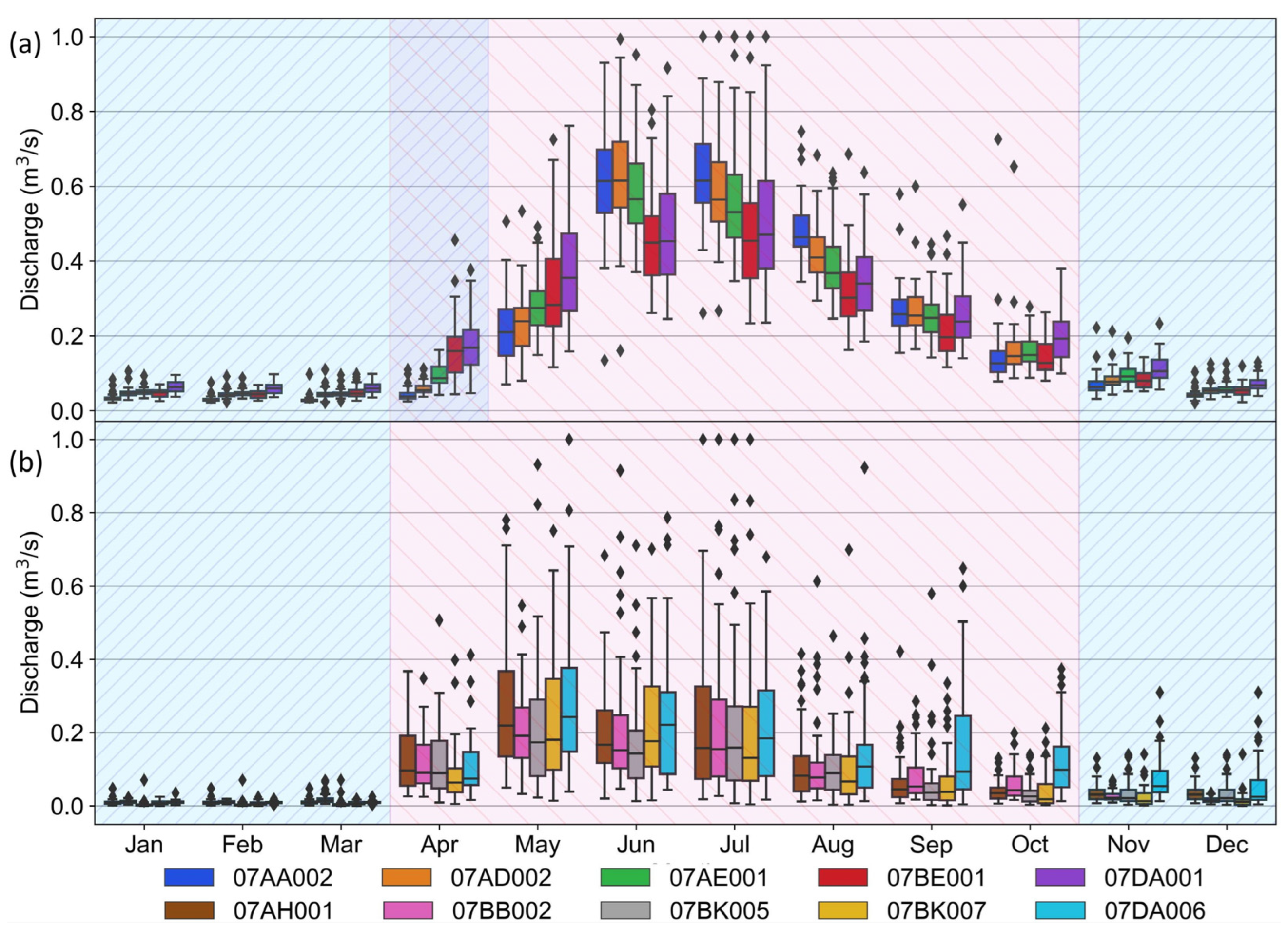
To define some threshold for ε, we divided our analysis into two sets of months, namely, cold months and (open) warm months. Figure 2 demonstrates averaged normalized monthly streamflow data distribution for the train and test sets. It can be observed from this figure that different cold months and (open) warm months may need to be considered for each of these stations due to substantial differences in average streamflow for each month. For the training data, according to Figure 2a, the month of April can be regarded as a warm month for 07BE001 and 07DA001; however, for the rest of the stations considered for this study, this month can be considered a cold month. Consequently, for 07AA002, 07AD002, and 07AE001, January, February, March, April, November, and December are considered to be cold months, and May, June, July, August, September, and October are regarded as warm months. Similarly, for the stations from the test set, according to Figure 2b, January, February, March, November, and December are regarded as cold months, while April, May, June, July, August, September, and October are regarded as warm months.
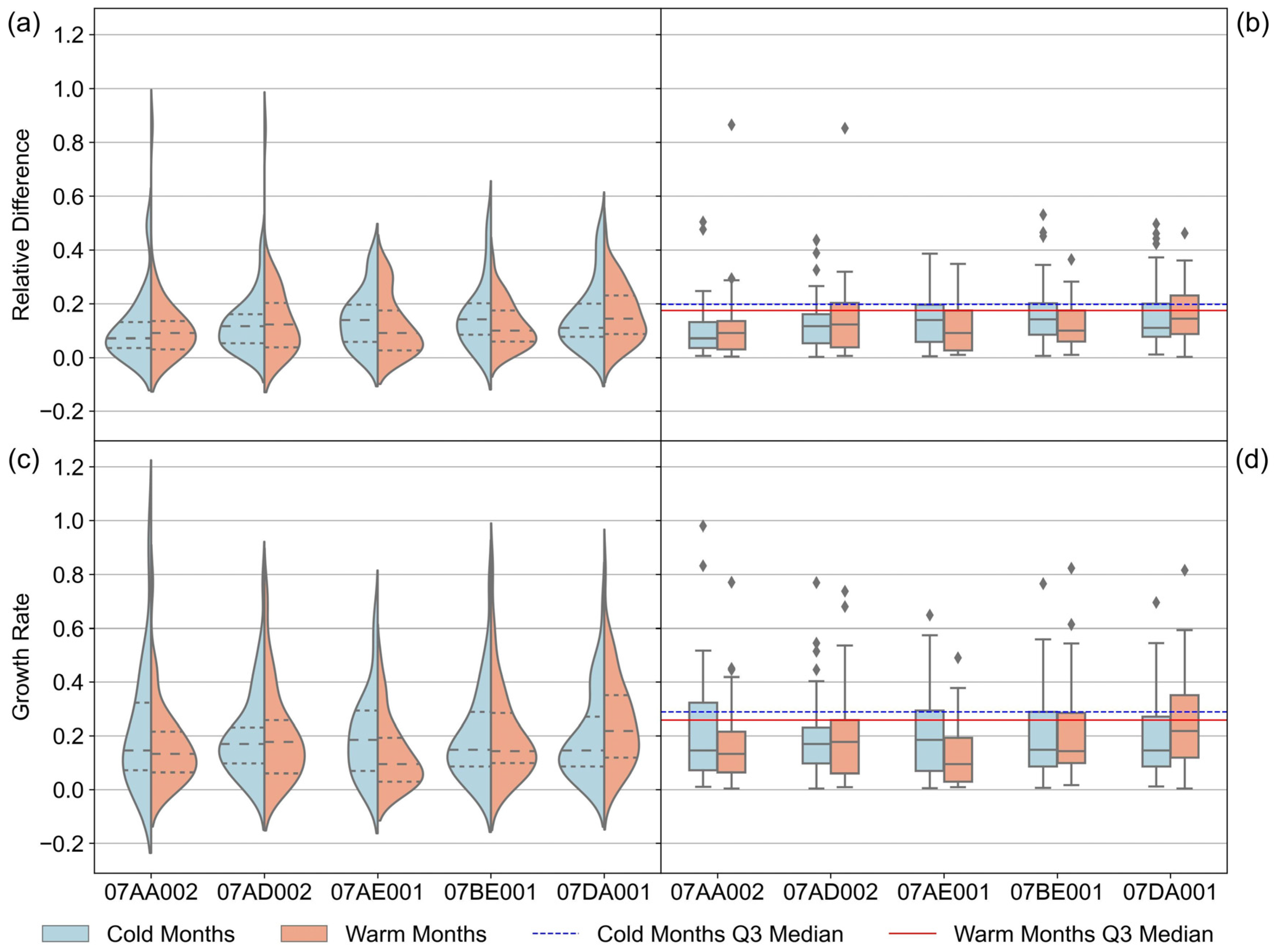
To identify ε thresholds from Algorithm 1 for each streamflow time series, we recorded all RD and GR values produced in each iteration for each station. Let denote a set containing all GR/RD values generated in all iterations of Algorithm 1 for each season (warm or cold) and each hydrometric station. For pinpointing the Relative Difference ε thresholds, observe that violin plots available in Figure 3a demonstrate probability density functions (PDF) [44,45,46] of each set, and the left side of each violin plot (shaded with blue) is responsible for the data distribution of set T for the cold months while the right side of each violin plot (shaded with pink) highlight the data distribution of set for the cold months. The bandwidth of these PDFs was calculated using Scott’s rule of thumb [47]. It is important to note that the probability density function is nonnegative everywhere, and the area under the whole curve equals one [48]. The three dashed lines on each side of each violin plot correspond to the lower edge, middle, and upper edge of their corresponding box plots available in Figure 3b. These dashed lines and box plots show the first quartiles (Q1), second quartiles (Q2), and third quartiles (Q3) [49] for each set , for the bottom to up direction, respectively. These three quartiles split the distribution into four equal successive subsets, and the second quartile (Q2) represents the median of each T set [49]. As for ε, based on our analysis and investigation, third quartiles (Q3) for each set were designated as thresholds. Growth Rate ε thresholds were also determined likewise using Figure 3c,d. Table 2 provides a summary of these ε thresholds.
| Algorithm 1 Regime Shift Change Detection (RSCD) algorithm, * Refine Method (RM). This parameter determines the two specializations of this method. ** xr is a point right after point c(j+1) |
| Input: , μ, σ, ε, and RM * Output: Periods P ← potential change point candidates through with 1 ≤ j ≤ n − 1; if n(Y) ≥ 2 then ← consecutive potential change point candidates; while n(C) ≥ 2 do for () do if there is a period after then if > then Remove from C else Remove from C end else if GR(, ) > GR(, ) ** then Remove from C else Remove from C end end end Update C end Update Y end if n(Y) ≥ 1 then ← periods defined using m change points; while n(P) ≥ 2 do for do if RM = Relative-Difference then if RD() < ε then Merge periods and end end if RM = Growth Rate then if GR() < ε then Merge periods and end end end Update P end else There is no regime shift. End |
These general ε thresholds were employed for testing the RSCD algorithm on the streamflow data for five hydrometric stations from the test set. As pointed out in Section 2.3.1, the longest continuous periods were chosen for these stations, and short gaps were filled utilizing interpolations. The available period of record between 1961–1990 was used to calculate µ and σ for test stations, as often monitoring record is not available for the entire baseline period (1961–1990).
2.3.4. RSCD for Newly Observed Data
Algorithm 1 can be adapted for usage on newly observed data which is paramount for the usage of this algorithm in comparative real-time. For a new set of observed data , the same µ and σ can be employed for determining candidate points as the reference baseline period would still be the same. As for thresholds, the same thresholds that were identified for each station in Table 2 (or the general threshold from Table 3 for cold and warm months) can be used. The primary difference would be how Growth Rate and Relative Difference refined methods utilized at this step. Since Relative Difference requires the maximum and minimum of set X, new data from set X* and previously observed data from X need to be taken into consideration. Therefore, if either max0≤i≤n {xi} or min0≤i≤n {xi} is smaller than some value from set X*, Algorithm 1 needs to be applied again on . However, using the RSCD with Growth Rate (RSCD-GR), only the newly observed data needs to be investigated.
3. Results
3.1. Seasonal Modeling and Gap Filling of Hydrometric Data Time Series
The acquired streamflow time series data were aggregated monthly. Some missing data points were observed in each aggregated dataset. The analysis completed in this study could be sensitive to the quality of the data. To ensure that these missing data were predicted accurately, Seasonal Autoregressive Integrated Moving Average (SARIMA) was used to develop models for each set using available data. SARIMA models in forwarding and backward directions were used for backcasting, forecasting, and filling gaps. By the end of this process, the streamflow time series associated with 07AD002 and 07BE001 were extended.
By investigations, we found that modeling through RFR can provide more promising results than SARIMA modeling for monthly aggregated streamflow datasets from 07AA002 and 07AE001. As a result, two separate multi-variable Random Forest Regression (RFR) models for predicting missing values of streamflow time series associated with 07AA002 and 07AE001 stations using streamflow time series from 07AD002, 07BE001, and 07DA001. In order to reduce the bias, fivefold cross-validation was used [50,51]. Table 3 illustrates the result of modeling using SARIMA and the Random Forest Regressor (RFR).
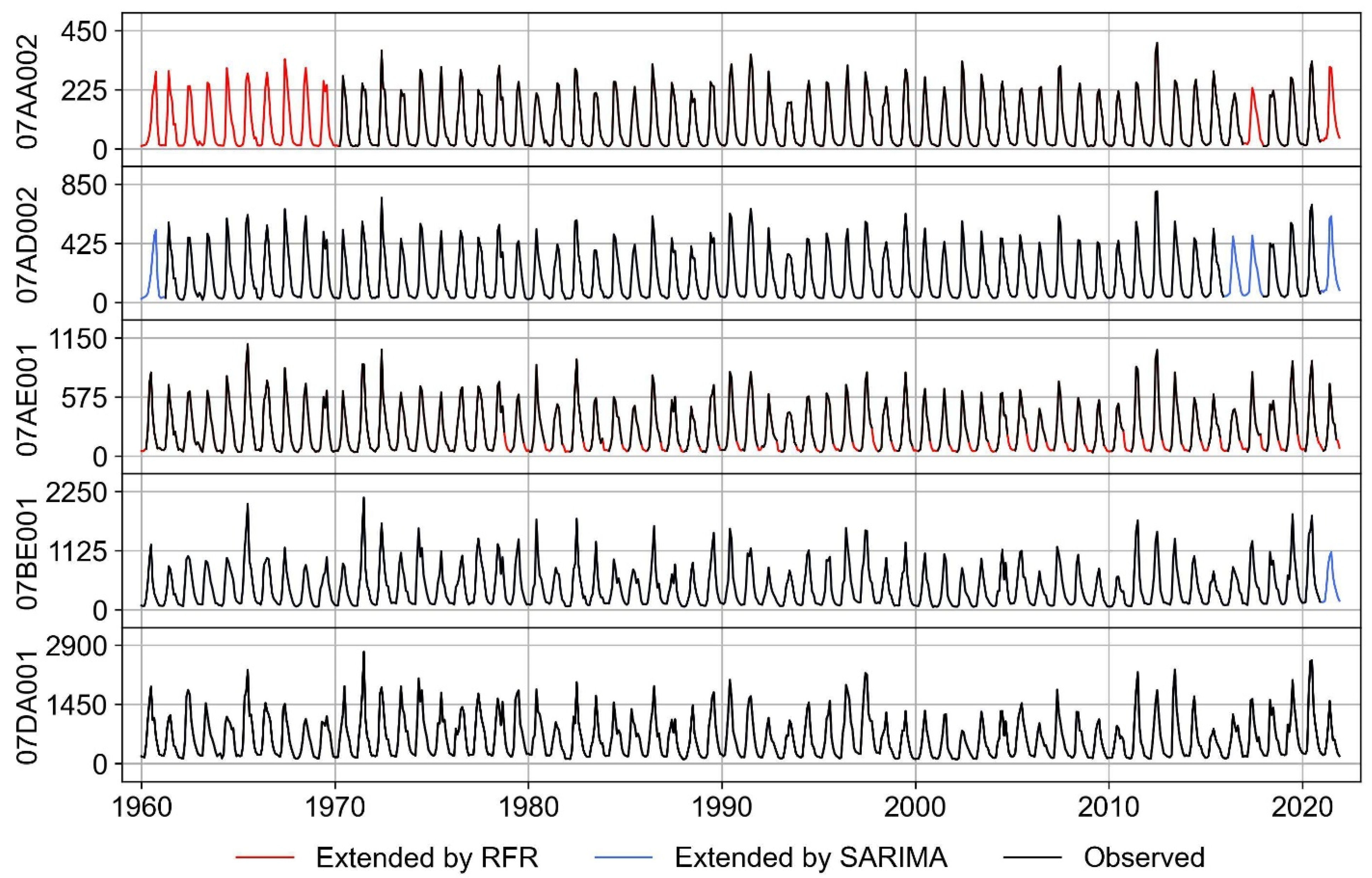
The observed and extended streamflow data using SARIMA and RFR modeling for 07AA002, 07AD002, 07AE001, 07BE001, and 07DA001 are available in Figure 4. In this figure, the observed/available streamflow data, extended streamflow data using SARIMA, and extended streamflow data using RFR are represented by solid black lines, solid blue lines, and solid red lines, respectively.
3.2. Regime Shift Change Detection (RSCD)
In this section, Algorithm 1 was applied to the streamflow time series extended by SARIMA and RFR from Section 3.1, where µ and σ were calculated using a baseline period 1961–1990 and ε thresholds from Table 2. As pointed out in Section 2.3.2, the months from April to October were considered warm months for 07BE001 and 07DA001, and the months from May to October were considered warm months for 07AA002, 07AD002, and 07AE001. The outputs of the RSCD algorithm using the same µ and σ and ε thresholds from Table 2 for both RSCD-RD and RSCD-GR were similar for the majority of the time series from the train set. We investigated a total of 60 time series, with 12 time series per station from the train set. Neither RSCD-RD nor RSCD-GR detected a regime shift in the 33 time series. For the nine time series, the same regime shifts detect. In the five time series, only RSCD-GR detected regime shifts, while in another six time series, only RSCD-RD detected regime shifts. Both methods detected regime shifts in seven time series, but the detections were slightly different.
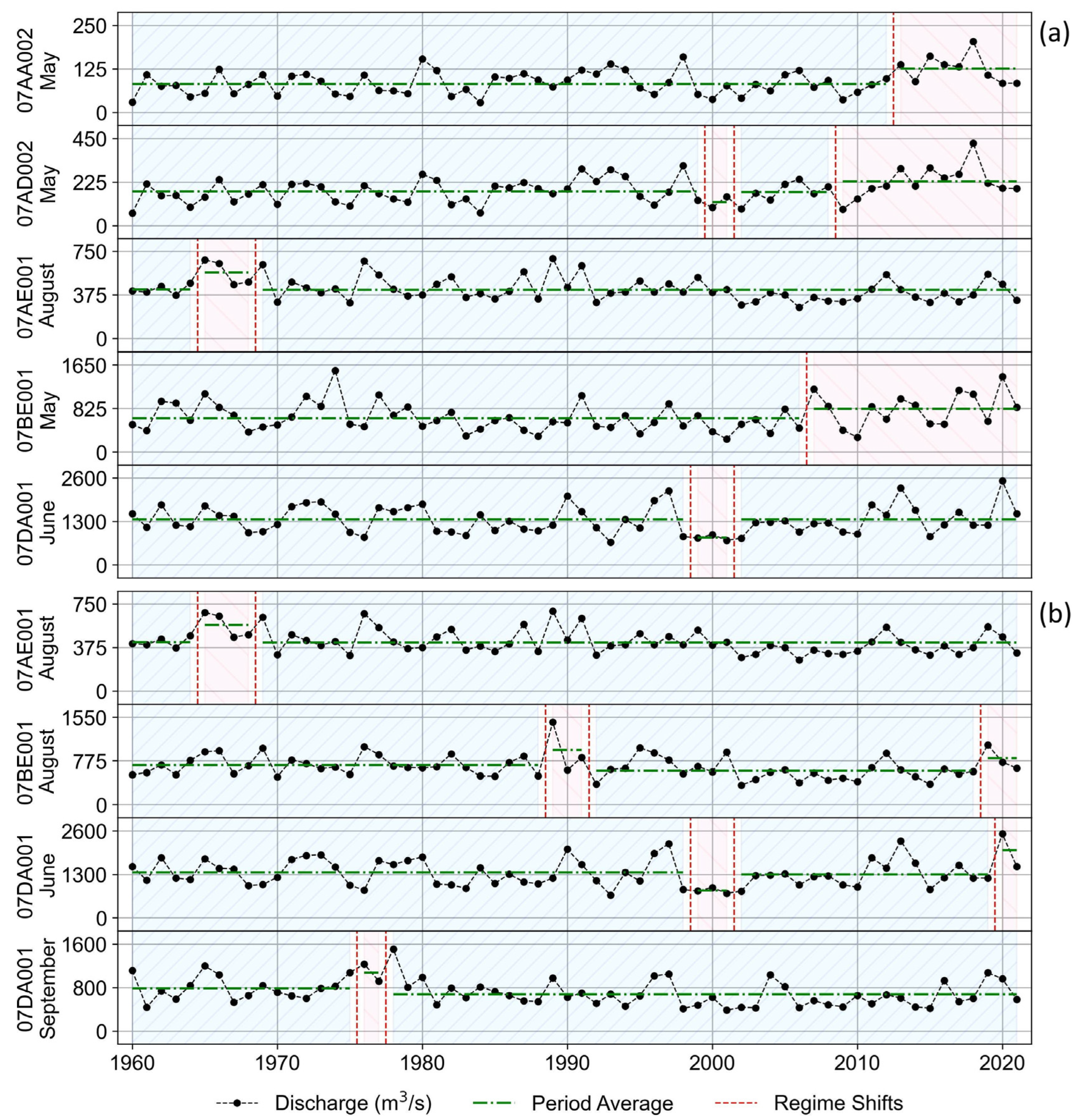
Figure 5 and Figure 6 highlight the output of RSCD-RD and RSCD-GR with the above settings for µ, σ, and ε for warm and cold months, respectively. Two criteria were used for the selection of these set months for presentation in Figure 5. First, whether some regime shift change was detected by the RSCD algorithm, and second, whether there were some differences between the output of RSCD-RD and RSCD-GR. The main idea was to highlight the key differences between RSCD-RD and RSCD-GR.
Figure 5a includes some periods that were identified by RSCD-GR but not by RSCD-RD. The streamflow fluctuations were greater during the warm months, as expected, and some of the identified periods were intriguing. For example, RSCD-GR identified two periods that appear to be correct for 07BE001 (May) and 07AA002. However, the period identified from 2000 to 2002 appears to be superfluous for 07AD002 (May). Similarly, Figure 5b has several periods detected by RSCD-RD but not by RSCD-GR. The identified periods were of a shorter duration: for example, 07AE001 (August), between 1965 and 1969, seems to be identified properly by RSCD-RD. In the middle ARB, 07BE001, a regime shift was identified in May 2007. However, at the beginning of the lower ARB, 07DA001, we did not identify a regime shift in the same month. We could assume that the streamflow at the beginning of the lower ARB increased. However, clear river water coming from the adjacent province, Saskatchewan, might have a lower stream flow. Another potential reason could be some water extracted from the river for industrial reasons. In either case, further investigations might be required.
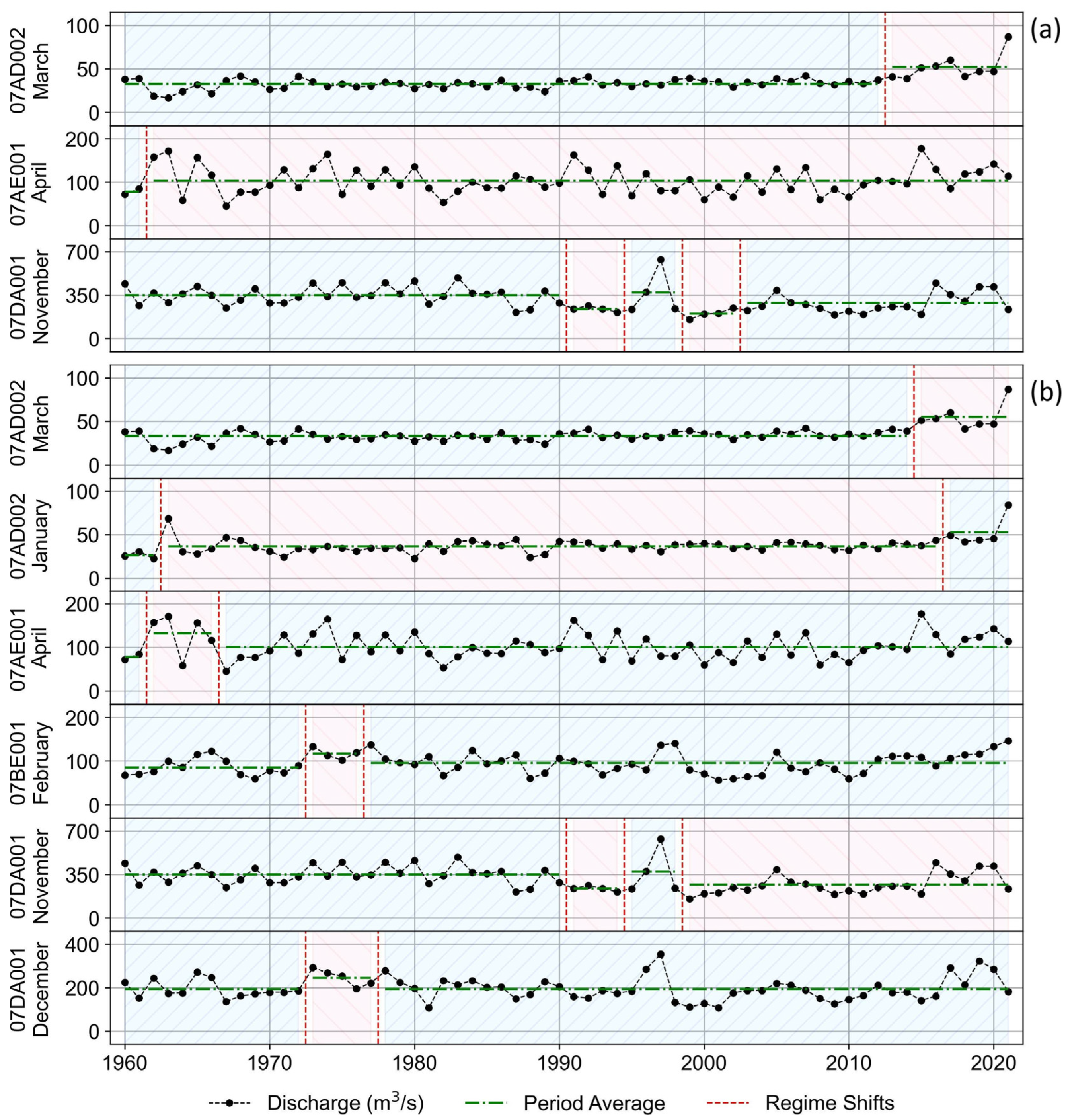
Figure 6a,b exhibit that the two periods identified by RSCD-GR and RSCD-RD were slightly mismatched for 07AD002 (March). Similarly, for 07AE001 (April), RSCD-GR identified two periods, whereas RSCD-RD detected three. Likewise, RSCD-GR found more periods than RSCD-RD for 07DA001 (November). There were some regime shifts during the cold months; however, flow changes within the month are insignificant.
3.3. RSCD Algorithm for the Test Set
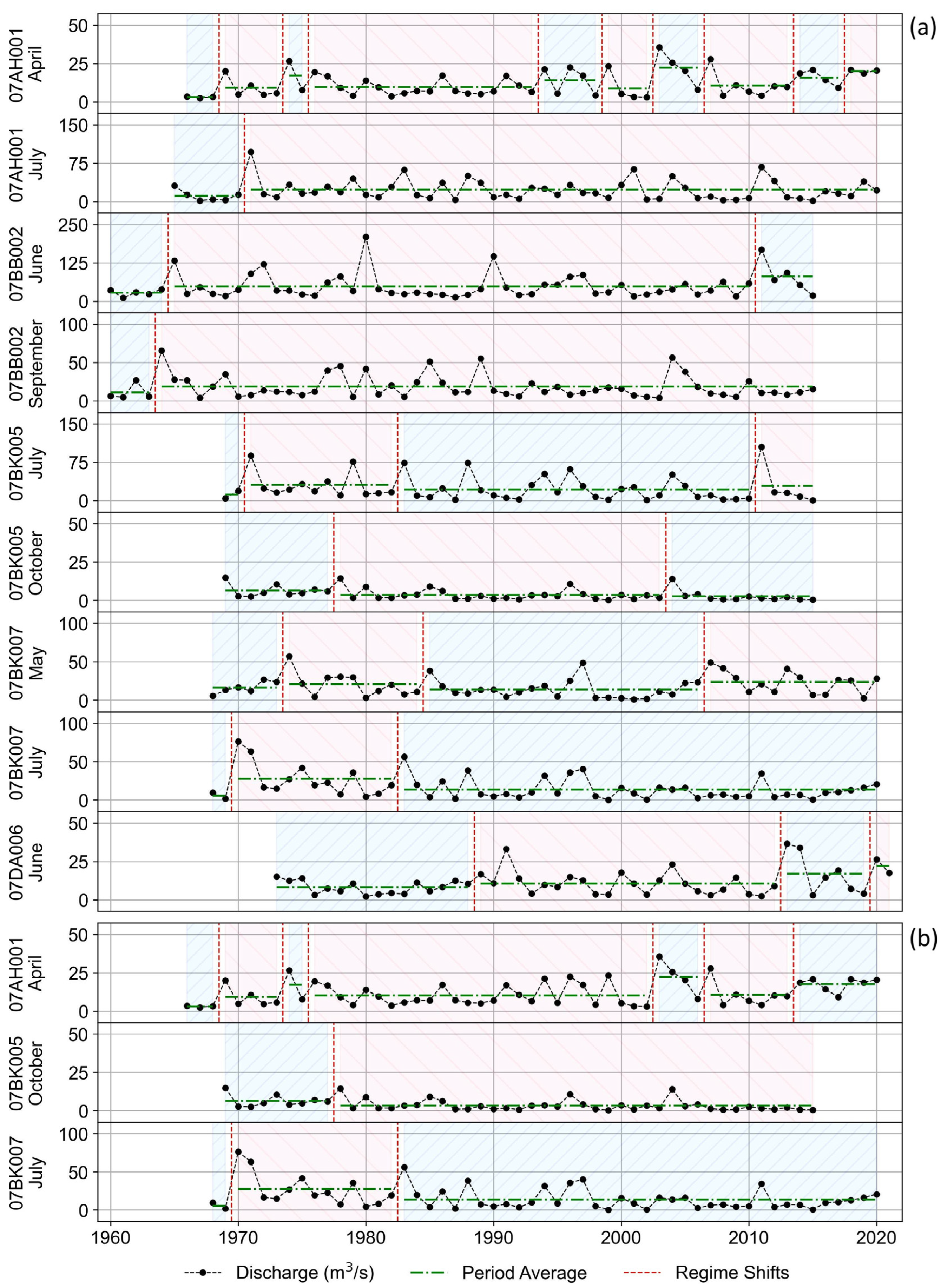
Figure 7 highlights RSCD Results for the test set using a 30-year (1961–1990) period for calculating µ and σ, general ε thresholds from Table 2, and RSCD-RD and RSCD-GR, respectively. General thresholds for the warm and cold seasons were used according to Figure 2b.
In the case of 07AH001 (April), RSCD-GR identified more periods than RSCD-RD. The same holds true for 07BK005 (October), where RSCD-GR identified more periods than RSCD-RD. Both methods generated the same results for 07BK007 (July). For the remaining months from Figure 6a, RSCD-GR identified those periods, yet RSCD-RD did not identify any. Correspondingly, we investigated 60 time series from the test set. In the nine time series, neither RSCD-RD nor RSCD-GR detected a regime shift. Identical regime shifts were detected in eight time series. In 40 time series, only RSCD-GR detected regime shifts, while in no time series, only RSCD-RD detected regime shifts. Both methods detected regime shifts in seven time series, but the detections were slightly different. Evidently, we primarily highlighted the differences in the output of the RSDC using these two refined methods; however, some of the additional periods and regime changes recognized through RSCD-GR appeared to be excessive, and RSCD-RD seemed to output more accurate results.
4. Discussion
Due to the importance of quality and accuracy of data for developing a Robust Regime Shift Change Detection (RSCD) Algorithm, Seasonal Autoregressive Integrated Moving Average (SARIMA) models and Random Forest Regression (RFR) method was used to extend the observed data for five stations from the train set. During our preliminary analysis, we discovered that the streamflow time series associated with stations 07AD002 and 07BE001 were great prospects for SARIMA modeling. These data sets were extended. Then, in addition to gap-free data from 07DA001, they were used for RFR modeling to extend the streamflow time series data from 07AA002 and 07AE001 stations. Table 3 and Figure 4 summarize the output of these methods in terms of accuracy and identify in which periods these extensions took place. As per Table 3, SARIMA provided a more reliable model for the streamflow data from 07AD002 than that of 07BE001. However, this could be due to the more fluctuating nature of observed data for 07BE001 in comparison to that of 07AD002. In addition to the significance of the quality and precision of data, we made sure that the period 1961–1990, indicated by Carter et al. [43], was available in all these observed/extended streamflow data for preparing the RSCD algorithm.
The RSCD algorithm takes a set associated with a time series whose elements appear in consecutive order over some period of time , given mean µ and standard deviation σ values and a threshold ε for refining methods (Relative Difference and Growth Rate), and outputs a set which consist of periods. Although we determined the period 1961–1990 as a baseline period and calculated µ and σ using this period, with analysis and further considerations, another period can be chosen as the baseline period.
In using Figure 2, the months from April to October were deemed as warm months for 07BE001 and 07DA001, while the months from May to October were regarded as warm months for 07AA002, 07AD002, and 07AE001. Using the baseline period 1961–1990 that µ and σ are calculated upon, ε thresholds from Table 2, the output of RSCD-RD and RSCD-GR were roughly comparable for training stations. Figure 7 displayed the RSCD results for the test set using a 30-year (1961–1990) period for calculating µ and σ, and ε thresholds from Table 2. When general ε thresholds were employed on time-series data from the test set, the RSCD-RD looked significantly better in some cases. We primarily highlighted the months and stations that demonstrate substantial dissimilarities between these two methods. Nonetheless, this exhibited some of the downsides of RSCD-GR as it might not perform as well as RSCD-RD on untrained data. The main reason behind this difference can be found in Figure 3. The probability density functions (PDF) for Relative Difference (both Cold and Warm months) were denser than those of Growth Rate around the median of each set T. Likewise, as it was visible in panels (b) and (d) from Figure 3, the average distance between the medians and the Q3 quartiles for Relative Difference was a bit less than those of the Growth Rate. Therefore, theoretically speaking, a median of these Q3 quartiles, which is here considered a general threshold, should work better for RSCD-RD. In other words, the RSCD-GR might need to be trained to identify a specific ε threshold for each cold and warm month. If the total observed data is not excessively large, we recommend using RSCD-RD instead of RSCD-GR because it may perform better.
One of the key advantages of the RSCD-GR over the RSCD-RD is the way it treats newly observed data. Using either RSCD-RD or RSCD-GR on a new set of observed data, the same µ and σ could be employed for determining candidate points. However, due to the definition of Relative Difference, if either the maximum/minimum of the newly observed data X* is large/smaller than those of the original set X, then all data points, i.e., , are required to be investigated again using RSCD-RD. For the RSCD-GR, newly observed data could be investigated separately, regardless.
Some of the challenges that we faced during this study was a lack of long continuous streamflow data, which was consequential for identifying regime shift changes. This issue was tackled for the streamflow data from hydrometric stations designated for training the RSCD algorithm; however, further investigation may be required to draw a conclusion about a relationship between almost all time series associated with hydrometric stations from the ARB region. Furthermore, the baseline period selected for this study is from 1961 to 1990; however, some of the hydrometric stations, especially from the lower ARB, initiated their data collection in the late 1990s or 2000s. Additional analyses are required to identify a baseline period for those hydrometric stations.
5. Conclusions
This study desired to propose a new robust Regime Shift Change Detection (RSCD) algorithm. The new proposed algorithm does not require any assumption on the length of each period for identifying regime changes. The analysis for purposing the RSCD algorithm could be susceptible to the quality of the data. This modeling and gap filling of hydrometric data time series were done by employing Seasonal Autoregressive Integrated Moving Average (SARIMA) models and Random Forest Regression (RFR) method, and short gaps in 07DA001 were filled through interpolation methods. The streamflow time series associated with 07AD002 and 07BE001 were extended by SARIMA modeling. Then gap-free data from 07AD002, 07BE001, and 07DA001 were utilized in concurrence with the RFR method to extend the streamflow time series associated with 07AA002 and 07AE001 stations.
The RSCD algorithm takes a time series, a given mean and standard deviation values, for a subset of this time series, and a threshold ε for refining methods, Relative Difference (RD), and Growth Rate (GR), outputs a set of periods. Even though the period 1961–1990 was chosen in this study as a baseline period, and the mean and standard deviation values were calculated using this period, with analysis and further considerations, other baseline periods can be chosen as well. Both RSCD-GR and RSCD-RD performed similarly in recognizing regime changes when threshold ε was pinpointed for each station and season (cold and warm); nonetheless, when it comes to testing set and using general thresholds for cold and warm months, the RSCD-RD performed substantially more favorable. One of the main strengths of RSCD-GR, over RSCD-RD, is that newly observed data can be investigated separately regardless, whereas for RSCD-RD, in some cases, the entire historical data needs to be re-investigated.
In May 2007, a regime change was found in the middle ARB, 07BE001. Nonetheless, at the beginning of the lower ARB, 07DA001, we did not discover a regime shift in the month of May. We could presume that the streamflow did rise at the beginning of the lower ARB; nevertheless, clear river water from the neighboring province of Saskatchewan could have a lower stream flow. Another possible explanation is that some river water was removed for industrial applications. In either situation, more study may be necessary.
The proposed general thresholds in this article were considered for the ARB region. With proper assumptions regarding cold and warm months, new thresholds can be obtained for other regions. An extension of this work could be applying this method to other regions and comparing the new general thresholds with those available from this study.
Author Contributions
Conceptualization, H.D., Q.K.H., A.G. and G.A.; methodology, H.D.; software, H.D.; validation, H.D., Q.K.H. and A.G.; formal analysis, H.D.; investigation, H.D.; resources, Q.K.H., A.G. and G.A.; data curation, H.D.; writing—original draft preparation, H.D.; writing—review and editing, H.D., Q.K.H. and G.A.; visualization, H.D.; supervision, Q.K.H.; project administration, Q.K.H.; funding acquisition, Q.K.H., G.A. and A.G. All authors have read and agreed to the published version of the manuscript.
Funding
This research was funded under Oil Sands Monitoring (OSM) Program. It was independent of any position of the OSM Program. The fund was awarded to Q.K.H. having an agreement number of 20GRAEM04.
Data Availability Statement
The data used in this research are available in the public domain.
Acknowledgments
The authors would like to thank the Water Survey of Canada (WSC) for the river streamflow (discharge) data used in this research.
Conflicts of Interest
The authors declare no conflict of interest.
Abbreviations
The following abbreviations are used in this manuscript:
| ARB | Athabasca River Basin |
| ARIMA | Autoregressive Integrated Moving Average |
| GR | Growth Rate |
| MA | Moving-Average |
| RFR | Random Forest Regressor |
| RSCD | Regime Shift Change Detection |
| RD | Relative Difference |
| RSCD-GR | RSCD with Growth Rate |
| RSCD-RD | RSCD with Relative Difference |
| SARIMA | Seasonal Autoregressive Integrated Moving Average |
| SRTM | Shuttle Radar Topography Mission |
| RAMP | The Regional Aquatics Monitoring Program |
| WSC | Water Survey of Canada |
References
- Myronidis, D.; Fotakis, D.; Ioannou, K.; Sgouropoulou, K. Comparison of ten notable meteorological drought indices on tracking the effect of drought on streamflow. Hydrol. Sci. J. 2018, 63, 2005–2019. [Google Scholar] [CrossRef]
- Zaghloul, M.S.; Ghaderpour, E.; Dastour, H.; Farjad, B.; Gupta, A.; Eum, H.; Achari, G.; Hassan, Q.K. Long Term Trend Analysis of River Flow and Climate in Northern Canada. Hydrology 2022, 9, 197. [Google Scholar] [CrossRef]
- Jiongxin, X. The water fluxes of the Yellow River to the sea in the past 50 years, in response to climate change and human activities. Environ. Manag. 2005, 35, 620–631. [Google Scholar] [CrossRef] [PubMed]
- Zhao, G.; Li, E.; Mu, X.; Wen, Z.; Rayburg, S.; Tian, P. Changing trends and regime shift of streamflow in the Yellow River basin. Stoch. Environ. Res. Risk Assess. 2015, 29, 1331–1343. [Google Scholar] [CrossRef]
- Burke, A.R.; Kasahara, T. Subsurface lateral flow generation in aspen and conifer-dominated hillslopes of a first order catchment in northern Utah. Hydrol. Process. 2011, 25, 1407–1417. [Google Scholar] [CrossRef]
- Godsey, S.E.; Kirchner, J.W.; Tague, C.L. Effects of changes in winter snowpacks on summer low flows: Case studies in the Sierra Nevada, California, USA. Hydrol. Process. 2014, 28, 5048–5064. [Google Scholar] [CrossRef]
- Tang, G.; Li, S.; Yang, M.; Xu, Z.; Liu, Y.; Gu, H. Streamflow response to snow regime shift associated with climate variability in four mountain watersheds in the US Great Basin. J. Hydrol. 2019, 573, 255–266. [Google Scholar] [CrossRef]
- Rostami, S.; He, J.; Hassan, Q.K. Water quality response to river flow regime at three major rivers in Alberta. Water Qual. Res. J. 2020, 55, 79–92. [Google Scholar] [CrossRef]
- Aminikhanghahi, S.; Cook, D.J. A survey of methods for time series change point detection. Knowl. Inf. Syst. 2017, 51, 339–367. [Google Scholar] [CrossRef]
- Zhu, Z. Change detection using landsat time series: A review of frequencies, preprocessing, algorithms, and applications. ISPRS J. Photogramm. Remote Sens. 2017, 130, 370–384. [Google Scholar] [CrossRef]
- Rodionov, S. A brief overview of the regime shift detection methods, Large-Scale Disturbances (Regime Shifts) and Recovery in Aquatic ecosystems: Challenges for Management Toward Sustainability. In Proceedings of the UNESCO-ROSTE/BAS Workshop on Regime Shifts, Varna, Bulgaria, 14–16 June 2005; pp. 17–24. [Google Scholar]
- Goossens, C.; Berger, A. How to recognize an abrupt climatic change? In Abrupt Climatic Change; Springer: Berlin/Heidelberg, Germany, 1987; pp. 31–45. [Google Scholar]
- Pettitt, A.N. A non-parametric approach to the change-point problem. J. R. Stat. Soc. Ser. C (Appl. Stat.) 1979, 28, 126–135. [Google Scholar] [CrossRef]
- Chu, P.S.; Zhao, X. Bayesian change-point analysis of tropical cyclone activity: The central North Pacific case. J. Clim. 2004, 17, 4893–4901. [Google Scholar] [CrossRef]
- Karl, T.R.; Williams, C.N. An Approach to Adjusting Climatological Time Series for Discontinuous Inhomogeneities. J. Appl. Meteorol. 1987, 26, 1744–1763. [Google Scholar] [CrossRef]
- Basseville, M.; Nikiforov, I.V. Detection of Abrupt Changes: Theory and Application; Prentice Hall: Englewood Cliffs, NJ, USA, 1993; Volume 104. [Google Scholar]
- Solow, A.R. Testing for climate change: An application of the two-phase regression model. J. Appl. Meteorol. Climatol. 1987, 26, 1401–1405. [Google Scholar] [CrossRef]
- Storch, H.v. Misuses of statistical analysis in climate research. In Analysis of Climate Variability; Springer: Berlin/Heidelberg, Germany, 1999; pp. 11–26. [Google Scholar]
- Wang, F.; Zhao, G.; Mu, X.; Gao, P.; Sun, W. Regime shift identification of runoff and sediment loads in the Yellow River Basin, China. Water 2014, 6, 3012–3032. [Google Scholar] [CrossRef]
- Khan, M.; Dahal, V.; Jeong, H.; Markus, M.; Bhattarai, R. Relative Contribution of Climate Change and Anthropogenic Activities to Streamflow Alterations in Illinois. Water 2021, 13, 3226. [Google Scholar] [CrossRef]
- Hamed, K.H.; Rao, A.R. A modified Mann-Kendall trend test for autocorrelated data. J. Hydrol. 1998, 204, 182–196. [Google Scholar] [CrossRef]
- Taylor, W. A Pattern Test for Distinguishing between Autoregressive and Mean-Shift Data; Taylor Enterprises: Libertyville, IL, USA, 2000; pp. 1–14. [Google Scholar]
- Rodionov, S. A sequential method of detecting abrupt changes in the correlation coefficient and its application to Bering Sea climate. Climate 2015, 3, 474–491. [Google Scholar] [CrossRef]
- Rodionov, S.N. A comparison of two methods for detecting abrupt changes in the variance of climatic time series. Adv. Stat. Climatol. Meteorol. Oceanogr. 2016, 2, 63–78. [Google Scholar] [CrossRef]
- Afrin, S.; Gupta, A.; Farjad, B.; Ahmed, M.R.; Achari, G.; Hassan, Q.K. Development of land-use/land-cover maps using Landsat-8 and MODIS data, and their integration for hydro-ecological applications. Sensors 2019, 19, 4891. [Google Scholar] [CrossRef]
- Meshesha, T.W.; Wang, J.; Melaku, N.D.; McClain, C.N. Modelling groundwater quality of the Athabasca River Basin in the subarctic region using a modified SWAT model. Sci. Rep. 2021, 11, 13574. [Google Scholar] [CrossRef]
- Shrestha, N.K.; Wang, J. Current and future hot-spots and hot-moments of nitrous oxide emission in a cold climate river basin. Environ. Pollut. 2018, 239, 648–660. [Google Scholar] [CrossRef]
- Shrestha, N.K.; Du, X.; Wang, J. Assessing climate change impacts on fresh water resources of the Athabasca River Basin, Canada. Sci. Total Environ. 2017, 601, 425–440. [Google Scholar] [CrossRef] [PubMed]
- Hatfield Consultants; Kilgour & Associates Ltd.; Klohn Crippen Berger Ltd.; Western Resource Solutions. RAMP: Technical design and Rationale. 2009. Available online: ramp-alberta.org (accessed on 2 February 2023).
- Box, G.E.P.; Jenkins, G.M.; Bacon, D.W. Models for Forecasting Seasonal and Non-Seasonal Time Series; University of Wisconsin Madison—Department of Statistics: Madison, WI, USA, 1967. [Google Scholar]
- Box, G.E.P.; Pierce, D.A. Distribution of Residual Autocorrelations in Autoregressive-Integrated Moving Average Time Series Models. J. Am. Stat. Assoc. 1970, 65, 1509–1526. [Google Scholar] [CrossRef]
- Breiman, L. Rejoinder: Arcing classifiers. Ann. Stat. 1998, 26, 841–849. [Google Scholar] [CrossRef]
- Buitinck, L.; Louppe, G.; Blondel, M.; Pedregosa, F.; Mueller, A.; Grisel, O.; Niculae, V.; Prettenhofer, P.; Gramfort, A.; Grobler, J.; et al. API design for machine learning software: Experiences from the scikit-learn project. In ECML PKDD Workshop: Languages for Data Mining and Machine Learning; MIT Press: Cambridge, MA, USA, 2013; pp. 108–122. [Google Scholar]
- Brockwell, P.J.; Davis, R.A. Time Series: Theory and Methods; Springer: New York, NY, USA, 1991. [Google Scholar]
- Hipel, K.W.; McLeod, A.I. Time Series Modelling of Water Resources and Environmental Systems; Elsevier: Amsterdam, The Netherlands, 1994. [Google Scholar]
- Dabral, P.; Murry, M.Z. Modelling and Forecasting of Rainfall Time Series Using SARIMA. Environ. Process. 2017, 4, 399–419. [Google Scholar] [CrossRef]
- Breiman, L. Random forests. Mach. Learn. 2001, 45, 5–32. [Google Scholar] [CrossRef]
- Rodriguez-Galiano, V.; Sanchez-Castillo, M.; Chica-Olmo, M.; Chica-Rivas, M. Machine learning predictive models for mineral prospectivity: An evaluation of neural networks, random forest, regression trees and support vector machines. Ore Geol. Rev. 2015, 71, 804–818. [Google Scholar] [CrossRef]
- Good, R.; Fletcher, H.J. Reporting explained variance. J. Res. Sci. Teach. 1981, 18, 1–7. [Google Scholar] [CrossRef]
- Willmott, C.J.; Matsuura, K. Advantages of the mean absolute error (MAE) over the root mean square error (RMSE) in assessing average model performance. Clim. Res. 2005, 30, 79–82. [Google Scholar] [CrossRef]
- Prasad, N.N.; Rao, J.N. The estimation of the mean squared error of small-area estimators. J. Am. Stat. Assoc. 1990, 85, 163–171. [Google Scholar] [CrossRef]
- Steel, R.G.D.; Torrie, J.H. Principles and procedures of statistics. In Principles and Procedures of Statistics; McGraw-Hill Book Company, Inc.: New York, NY, USA; Toronto, ON, Canada; London, UK, 1960. [Google Scholar]
- Carter, T.; Parry, M.; Harasawa, H.; Nishioka, S. IPCC technical guidelines for assessing climate change impacts and adaptations. In Part of the IPCC Special Report to the First Session of the Conference of the Parties to the UN Framework Convention on Climate Change, Intergovernmental Panel on Climate Change. Department of Geography, University College London, UK and Center for Global Environmental Research, National Institute for Environmental Studies, Tsukuba, Japan; Publications of the Natural Resources Institute Finland: Helsinki, Finland, 1994; Volume 59. [Google Scholar]
- Dastour, H.; Ghaderpour, E.; Hassan, Q.K. A Combined Approach for Monitoring Monthly Surface Water/Ice Dynamics of Lesser Slave Lake Via Earth Observation Data. IEEE J. Sel. Top. Appl. Earth Obs. Remote Sens. 2022, 15, 6402–6417. [Google Scholar] [CrossRef]
- Terrell, G.R.; Scott, D.W. Variable kernel density estimation. Ann. Stat. 1992, 20, 1236–1265. [Google Scholar] [CrossRef]
- Epanechnikov, V.A. Non-parametric estimation of a multivariate probability density. Theory Probab. Its Appl. 1969, 14, 153–158. [Google Scholar]
- Scott, D.W. Scott’s rule. Computational Statistics. Wiley Interdiscip. Rev. 2010, 2, 497–502. [Google Scholar] [CrossRef]
- Kozak, R.; Kozak, A.; Staudhammer, C.; Watts, S. Introductory Probability and Statistics, Revised Edition: Applications for Forestry and the Natural Sciences; CABI: Wallingford, UK, 2019. [Google Scholar]
- Han, J.; Kamber, M.; Pei, J. Getting to know your data. In Data Mining; Morgan Kaufmann: Boston, MA, USA, 2012; Volume 2, pp. 39–82. [Google Scholar]
- Shao, J. Linear model selection by cross-validation. J. Am. Stat. Assoc. 1993, 88, 486–494. [Google Scholar] [CrossRef]
- Schumacher, M.; Holländer, N.; Sauerbrei, W. Resampling and cross-validation techniques: A tool to reduce bias caused by model building? Stat. Med. 1997, 16, 2813–2827. [Google Scholar] [CrossRef]
Figure 1.
A map of the Athabasca River Basin (ARB). The gradient background color was produced using Shuttle Radar Topography Mission (SRTM) data sampled at 30 m. The right corner window demonstrates the location of the ARB within Canada. Stations selected for training the RSCD algorithm are exhibited with circles, whereas stations selected for testing the algorithm are illustrated with stars.

Figure 2.
Averaged normalized monthly streamflow data distribution by train (a) and test (b) sets. Cold months are highlighted with blue color, and warm months are shaded by pink color. In part (a), for the month of April, blue and pink colors are overlapped as this month was considered a warm month for 07BE001 and 07DA001 but a cold month for 07AA002, 07AD002, and 07AE001. For part (b), January, February, March, November, and December are regarded as cold months, while April, May, June, July, August, September, and October are considered as warm months.

Figure 3.
Set T distribution plot for each station separated by warm and cold months: (a,c) density data distribution for set T. (b,d) box plot data distribution for set T.
Figure 3.
Set T distribution plot for each station separated by warm and cold months: (a,c) density data distribution for set T. (b,d) box plot data distribution for set T.

Figure 4.
The observed and extended streamflow (m3/s) monthly time series through SARIMA (solid blue line) and RFR (solid red line) modeling for 07AA002 (Athabasca River near Jasper), 07AD002 (Athabasca River at Hinton), 07AE001 (Athabasca River near Windfall), 07BE001 (Athabasca River at Athabasca), and 07DA001 (Athabasca River below Fort McMurray).

Figure 5.
RSCD Results for warm months using Growth Rate (a), Relative Difference (b), and a 30-year (1961–1990) period for calculating µ and σ, and ε thresholds from Table 2. The streamflow (m3/s) is shown on the y-axis in each panel. The use of red and blue shades aids in distinguishing between the different regimes.

Figure 6.
RSCD Results for cold months using Growth Rate (a), Relative Difference (b), and a 30-year (1961–1990) period for calculating µ and σ, and ε thresholds from Table 2. The streamflow (m3/s) is shown on the y-axis in each panel. The use of red and blue shades aids in distinguishing between the different regimes.

Figure 7.
RSCD Results for warm and cold months using Growth Rate (a), Relative Difference (b), and a 30-year (1961–1990) period for calculating µ and σ, and ε thresholds from Table 2. The streamflow (m3/s) is shown on the y-axis in each panel. The use of red and blue shades aids in distinguishing between the different regimes.


Table 1.
Hydrometric stations used in this study.
| Set | ID | Name | Considered Period for This Study | Gross Drainage Area (km2) | Elevation (m) |
|---|---|---|---|---|---|
| 07AA002 | Athabasca River near Jasper | 1960–2021 | 3870 | 1041 | |
| 07AD002 | Athabasca River at Hinton | 1960–2021 | 9760 | 963 | |
| Train | 07AE001 | Athabasca River near Windfall | 1960–2021 | 19,600 | 735 |
| 07BE001 | Athabasca River at Athabasca | 1960–2021 | 74,600 | 513 | |
| 07DA001 | Athabasca River below Fort McMurray | 1960–2021 | 133,000 | 246 | |
| 07AH001 | Freeman River near Fort Assiniboine | 1965–2020 | 1660 | 661 | |
| 07BB002 | Pembina River near Entwistle | 1960–2015 | 4400 | 727 | |
| Test | 07BK005 | Saulteaux River near Spurfield | 1969–2015 | 2600 | 585 |
| 07BK007 | Driftwood River near the Mouth | 1968–2020 | 2100 | 569 | |
| 07DA006/S38 1 | Steepbank River near Fort McMurray | 1972–2021 | 1320 | 277 |
Note(s): 1 WSC and RAMP (The Regional Aquatics Monitoring Program (RAMP), 2022) dataset for this station were fused.
Table 2.
ε thresholds separated by cold and warm sets of months (seasons) for each hydrometric station. At the bottom part of the table, general thresholds are separated by cold and warm sets of months (seasons) for all hydrometric stations from the ARB region.
Table 2.
ε thresholds separated by cold and warm sets of months (seasons) for each hydrometric station. At the bottom part of the table, general thresholds are separated by cold and warm sets of months (seasons) for all hydrometric stations from the ARB region.
| ID | Season | Growth Rate ε | Relative Difference ε |
|---|---|---|---|
| 07AA002 | Cold | 0.322 | 0.130 |
| 07AA002 | Warm | 0.215 | 0.135 |
| 07AD002 | Cold | 0.231 | 0.160 |
| 07AD002 | Warm | 0.257 | 0.202 |
| 07AE001 | Cold | 0.293 | 0.197 |
| 07AE001 | Warm | 0.193 | 0.174 |
| 07BE001 | Cold | 0.288 | 0.202 |
| 07BE001 | Warm | 0.285 | 0.174 |
| 07DA001 | Cold | 0.271 | 0.200 |
| 07DA001 | Warm | 0.350 | 0.230 |
| General | Cold | 0.288 | 0.197 |
| General | Warm | 0.257 | 0.174 |
Table 3.
Accuracy test by various metrics for SARIMA modeling (07AD002 and 07BE001) and RFR modeling (07AA002 and 07AE001). The ideal value for Explained Variance Score (EVS) and the coefficient of determination (R2) is a number close to one, while the ideal value for the Mean Absolute Error (MAE) and the Mean Squared Error (MSE) is a number close to zero.
| Metrics | 07AA002 | 07AD002 | 07AE001 | 07BE001 |
|---|---|---|---|---|
| Train: EVS | 1.00 ± 2.32 × 10⁻⁴ | 0.901 | 0.99 ± 1.50 × 10⁻³ | 0.789 |
| Test: EVS | 0.98 ± 2.20 × 10⁻³ | 0.96 ± 4.15 × 10⁻² | ||
| Train: MAE | 2.89 ± 9.64 × 10⁻² | 30.692 | 9.74 ± 1.01 × 100 | 104.842 |
| Test: MAE | 7.60 ± 6.00 × 10⁻¹ | 27.83 ± 8.83 × 100 | ||
| Train: MSE | 23.16 ± 2.01 × 100 | 2982.181 | 294.80 ± 8.40 × 101 | 30,943.826 |
| Test: MSE | 159.69 ± 2.07 × 101 | 2563.86 ± 2.70 × 10³ | ||
| Train: R2 | 1.00 ± 2.32 × 10⁻⁴ | 0.901 | 0.99 ± 1.50 × 10⁻³ | 0.788 |
| Test: R2 | 0.98 ± 2.21 × 10⁻³ | 0.95 ± 4.31 × 10⁻² |
Disclaimer/Publisher’s Note: The statements, opinions and data contained in all publications are solely those of the individual author(s) and contributor(s) and not of MDPI and/or the editor(s). MDPI and/or the editor(s) disclaim responsibility for any injury to people or property resulting from any ideas, methods, instructions or products referred to in the content. |
© 2023 by the authors. Licensee MDPI, Basel, Switzerland. This article is an open access article distributed under the terms and conditions of the Creative Commons Attribution (CC BY) license (https://creativecommons.org/licenses/by/4.0/).
Share and Cite
MDPI and ACS Style
Dastour, H.; Gupta, A.; Achari, G.; Hassan, Q.K. A Robust Regime Shift Change Detection Algorithm for Water-Flow Dynamics. Water 2023, 15, 1571. https://doi.org/10.3390/w15081571
AMA Style
Dastour H, Gupta A, Achari G, Hassan QK. A Robust Regime Shift Change Detection Algorithm for Water-Flow Dynamics. Water. 2023; 15(8):1571. https://doi.org/10.3390/w15081571
Chicago/Turabian StyleDastour, Hatef, Anil Gupta, Gopal Achari, and Quazi K. Hassan. 2023. "A Robust Regime Shift Change Detection Algorithm for Water-Flow Dynamics" Water 15, no. 8: 1571. https://doi.org/10.3390/w15081571
Note that from the first issue of 2016, this journal uses article numbers instead of page numbers. See further details here.