Article

An Integrated Approach for Simulating Debris-Flow Dynamic Process Embedded with Physically Based Initiation and Entrainment Models

1
School of Civil Engineering, Central South University, Changsha 410075, China
2
Hunan Provincial Key Laboratory for Disaster Prevention and Mitigation of Rail Transit Engineering Structures, Changsha 410075, China
3
Department of Civil Engineering, Kyushu University, Fukuoka 819-0395, Japan
*
Author to whom correspondence should be addressed.
Water 2023, 15(8), 1592; https://doi.org/10.3390/w15081592
Submission received: 12 March 2023 / Revised: 6 April 2023 / Accepted: 18 April 2023 / Published: 19 April 2023
(This article belongs to the Section Water Erosion and Sediment Transport)

Abstract

:
Recent studies have indicated that the accurate simulation of debris flows depends not only on the selection of numerical models but also on the availability of precise data on the initial source location and depth. Unfortunately, it is currently difficult to obtain quantitative data on source locations and depths during field investigations or model experiments of debris flow disasters. Therefore, in this study, we propose an integrated approach for simulating the debris-flow dynamic process that includes the physically based slope initiation source estimation and the entrainment-incorporated process simulation. We treat the potential slip surfaces’ locations and depths as random variables to search for the critical surface corresponding to the minimum stability factor by Monte Carlo simulation. Using the spatial variation interval of the soil parameters, we estimate the range of possible critical slip surfaces and the interval of the initiation source volume. Moreover, we propose a wet/dry front treatment method applied to the finite difference scheme and integrate it into our entrainment-incorporated model to improve the stability and accuracy of the numerical solution over complex topography. The effectiveness of the method is demonstrated through a case study of the 2010 Hongchun debris flow event in Yingxiu town. The result indicates that our method is effective in simulating debris flow dynamics, including slope initiation source estimation and dynamic process simulation.

1. Introduction

Debris flow is a type of gravity-driven mass flow that occurs on steep gullies [1]. Sudden, fast-moving, and destructive, debris flows are the most common type of natural hazard in mountainous areas, posing a constant threat to structures, occupants, and the ecological environment. Evidence suggests that the hazard of debris flows is related to their runout extent and volume depth [2,3,4]. Therefore, the prediction of the runout extent and volume depth of debris flows is beneficial for debris flow disaster mitigation. This requires not only reasonable predictions of dynamic processes and bed-sediment entrainment along the path but also valid estimates of the location and depth of the slope initiation source in the source area.
There have been many studies on the mechanisms of debris flow slope source initiation [5]. These methods can be divided into three categories: field investigation, physical model experiments [6], and numerical simulation methods [7,8]. Field investigation is an important way to obtain information about the geological environment, initiation sources, and hydrological conditions in the study area. Combined with the investigation information, the causal mechanism and initiation mode of slope sources can be initially established. Physical model experiments mainly include field source site experiments and indoor model experiments [9]. Conventional physical experiments usually describe the slope source initiation process qualitatively based on the macroscopic instability damage phenomenon of the test material, and it is difficult to quantitatively obtain detailed results of the source stress, range, and depth. With the development of computer technology, the numerical simulation method based on mechanical analysis has become an important means to study slope source initiation.
According to model experiments and mechanism studies of landslide-to-debris flow transformation, many numerical simulation methods have been proposed for hillslope debris flow initiation mechanisms [7,10]. Some discrete media methods, such as the particle plow code method, have been used to simulate the source initiation and dynamic process of debris flows [11]. In terms of numerical simulation based on the continuous medium, some methods only set the outlet downstream of the debris-flow gully and simulate the input of flow mass based on the empirical flow curve [12,13]. In these methods, the flow curves and flow outlet locations are not easily predicted, which significantly affects the simulation results. Some methods artificially determine a region and a fixed depth in the source area as the initial source through field surveys or empirical assumptions [14,15]. In this case, the determination of the initial initiation fixed depth by field surveys or empirical assumptions is somehow subjective and lacks a theoretical basis.
For hillslope debris flow, in addition to the entrainment source along the path, the debris flow initiation process is mainly triggered by landslides caused by factors such as heavy rainfall or earthquakes [16]. Therefore, to estimate the extent and depth of slope sources based on physical mechanisms, stability analysis of slope unsaturated soils in the source area is required. In this regard, the limit equilibrium theory has been widely applied in many fields, which usually predetermines the slip surface and divides the soil into slices [17]. The stability of the slope source is determined by calculating the slip resistance and slip force of the slip surface. The slip surface with the smallest stability factor is the critical surface, which represents the area and depth of the initiation source and can be searched by methods such as the Swedish circle method and the Bishop method [18]. Many computational convenience methods apply only to the circular slip surface and can search the critical surface relatively efficiently. However, in the debris flow source area, there is obvious spatial variability in the soil parameters, which makes the slip surface compound shape, and the large scale of the slope body also increases the difficulty of searching the critical slip surface. For this kind of uncertainty, Monte Carlo simulation is a good solution, which is suitable for the quantitative analysis of complex systems by multiple random sampling as input parameters [19,20].
For the prediction of debris flow dynamic processes, numerical simulation is an effective solution that takes into account physical processes and usually treats the debris flow as a continuous medium [21,22]. Combined with the shallow-water assumption, many methods simplify the Navier–Stokes equations to shallow-water equations (SWEs) by depth integration, which are to serve as the governing equations for the debris flow dynamic process [23]. To obtain the variation in the debris flow depth and velocity with time and space, various numerical schemes in computational fluid dynamics are applied to solve the governing equations based on SWEs. Most of the numerical schemes can be typically classified into the finite difference method (FDM) [24,25] and the finite volume method (FVM) [26]. To discretize the governing equations, FDM replaces the differentiation by difference quotients of the function values of the nodes on the difference grids (structured grids), while FVM performs the integration of the governing equations within the subdivided control volumes, which can be structured or unstructured grids. With recent developments, continuum-based models have become the most widely used method in debris flow simulation.
However, there are still some problems in achieving a stable and accurate simulation of debris flow propagation. An essential issue is the numerical treatment of the wet/dry front since the wet/dry front moves continuously with time and elevation during the debris-flow process [27]. At the wet/dry fronts, the debris flow depth is usually very small, even close to zero, which poses a challenge to the accurate and stable solution of the numerical models. When the flow depth falls below a predefined threshold, some approaches empirically set the flow depth and associated cell velocity to zero, often resulting in an unexpected loss of debris flow mass and momentum. Others assume that the entire computational domain is covered by a pseudo-thin mass, which can increase the stability of the calculation [28]. However, the influence of cell surface levels on the migration of wet/dry fronts is easily neglected. A better approach is to employ wet/dry checking routines based on flow depth as well as surface levels, which should be comprehensively incorporated into the adopted numerical scheme [29].
To date, many wet/dry front treatment methods have been developed and applied in the simulation of earth surface flow processes [30]. These proposed methods can be broadly classified into three categories, i.e., the cell removal method [31,32], the slot method [33], and the thin film method [34]. The cell removal method uses the geometric or physical parameters of the cells to synthetically determine the wet/dry conditions of the cells and the manner in which the cells are calculated. Due to the flexibility of wet/dry cell handling and computational efficiency, this type of method has become the most widely used and efficient. Most of the methods tend to be highly specific to the numerical model they serve and are therefore difficult to apply to other types of numerical schemes [30]. Most of these established approaches are only applicable to the FVM scheme in conjunction with flux computations and various Riemann solvers and have been well validated [35]. However, as for the FDM scheme, systematic and efficient methods are rarely reported. Since FDM is free to deal with fluxes and Riemann solvers, it is difficult to apply the methods applicable to FVM schemes to the FDM scheme.
This paper presents an integrated approach for simulating debris-flow dynamics, encompassing the physically based initiation slope source estimation and the simulation of the entrainment-incorporated process. Our method employs Monte Carlo simulation to identify the critical surface of composite shape by considering the location and depth of the source slip surface as random variables. To account for the spatial variability of slope soil, we generate a sufficient dataset of input soil parameters to obtain the range of critical slip surface and initiation source volume. We also propose a wet/dry front treatment method applied to the finite difference method (FDM) and integrate it into our entrainment-incorporated model to enhance the stability and accuracy of the numerical solution. To evaluate the effectiveness and performance of our method, we apply it to the 2010 Hongchun debris-flow event as a case study.

2. Physically Based Initiation Model of the Debris Flow Sources

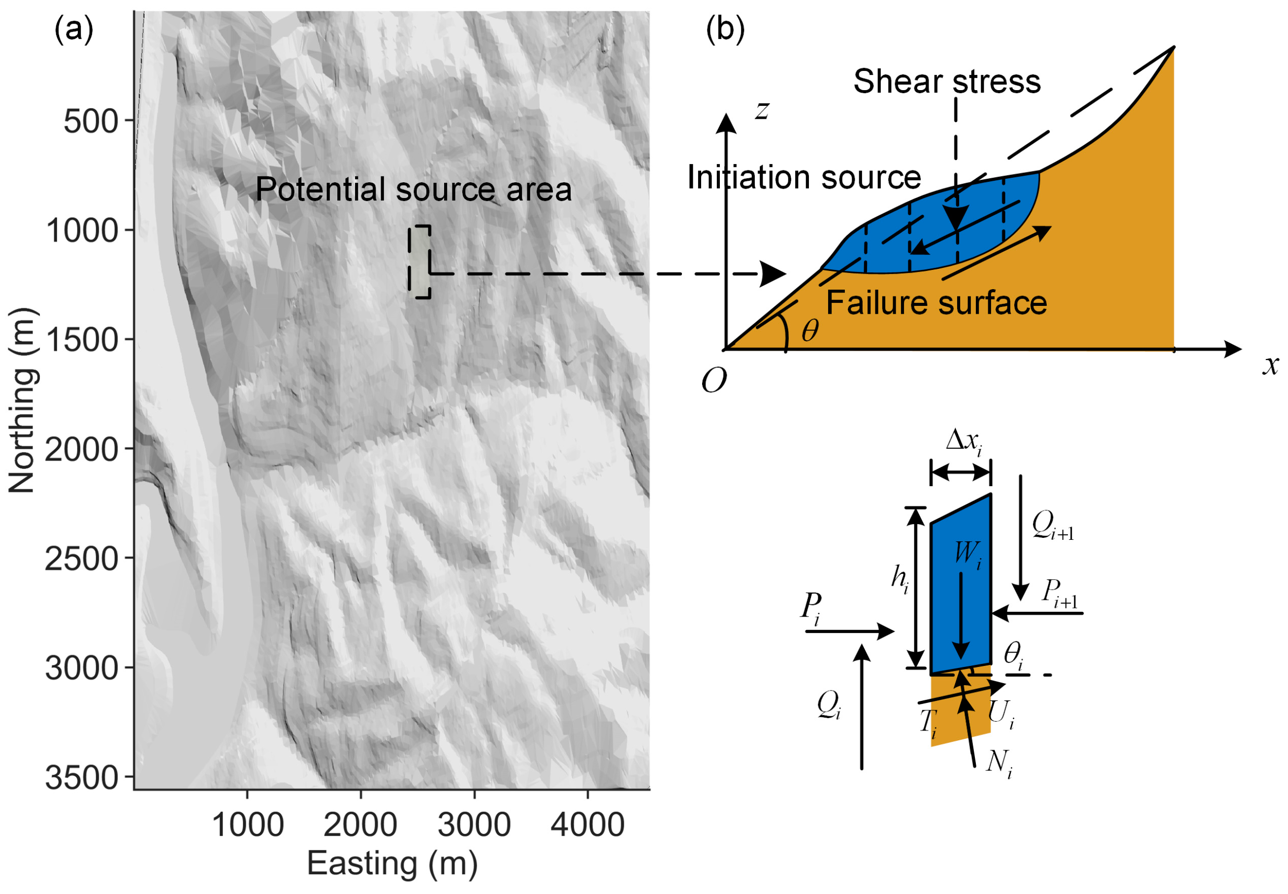
2.1. Limit Equilibrium Method for Slope Stability Analysis

Debris-flow disasters on slopes are typically caused by the destabilization of slope soil, which slides down the slope, resulting in landslides in the source area. The major mechanism lies in the increase in pore water pressure induced by soil seepage and the decrease in cohesion caused by earthquakes. As a result, the shear strength in the slope soil becomes lesser than the shear stress, ultimately resulting in large-scale shear damage. Over the topography before the occurrence of debris flow, the slip surface of the landslide can be used to determine the initiation location and depth of the debris flow source. In this paper, the limit equilibrium method is used to examine the slope stability of the potential source area, as illustrated in Figure 1. Since the width of debris flow gullies is usually much smaller than the length, we calculate the average surface elevation in the source area along the vertical gully direction.
The limit equilibrium theory assumes that when the landslide occurs, all points on the slip surface are in the state of limit equilibrium, and the failure surface is the critical surface [36]. The soil is assumed to exhibit a rigid-plastic behavior, and the strength is governed by the Moore–Coulomb damage criterion. To facilitate the calculation of slip resistance and slip force on the slip surface, the slope is usually divided into slices along the direction of gravity. As shown in Figure 1b, the elevation of the slope surface is represented as s ( x ) ( x 0 x x n ) , and the critical slip surface consists of a series of slice sub-nodes { c ( x ) | ( x 0 , z 0 ) , ( x 1 , z 1 ) , , ( x n , z n ) } .
The limit equilibrium method assumes that the forces between adjacent soil slices are balanced in magnitude and opposite in direction and that they act along the same line. Consequently, the method usually disregards the effect of inter-slice forces on the overall stability of the soil slope. The stability factor of the critical slip surface can be calculated as follows.
W i = 1 2 γ i [ s ( x i ) + s ( x i 1 ) z i z i 1 ] ( x i x i 1 )
l i = ( x i x i 1 ) 2 + ( z i z i 1 ) 2
F s = i = 1 n c i l i f i + i = 1 n W i ( 1 λ i ) c o s α i t a n φ i f i i = 1 n W i s i n α i
where c i , φ i and γ i represent the effective cohesion, internal friction angle, and unit weight of soil slice i , respectively; λ i is the pore pressure coefficient, which is the ratio of pore water pressure to normal stress; W i represents the gravity of soil slice i ; α i is the angle between the lower surface of the slice and the horizontal plane; f i is the slip determination parameter, which is equal to 1 unless the height of the slip slice is zero.
For homogeneous cohesive soil, the critical slip surface is usually circular or logarithmic spiral-type and can be searched by the Swedish circular method [18]. The center of the initial circular slip surface is determined from the table, and the stability factor can be calculated based on Equations (1)–(3). Then, the center of the circle is moved by the specified direction and step length until the stability factor is close to the minimum value concerning the critical slip surface.
Considering a homogeneous soil slope with c = 5   kPa , φ = 25 ° , γ = 20   kN / m 3 , and λ = 0.05 , the critical slip surface can be searched, as shown in Figure 2. For this critical slip surface, sensitivity analysis of each soil strength parameter is performed to evaluate the effect of variations in the input parameters on the slope stability factor. All the soil parameters are held constant except the one selected for the sensitivity analysis. From Figure 3, the stability factors are quite sensitive to the variation in all four strength parameters, where the increase in the soil pore pressure coefficient causes the slope stability to decrease significantly.

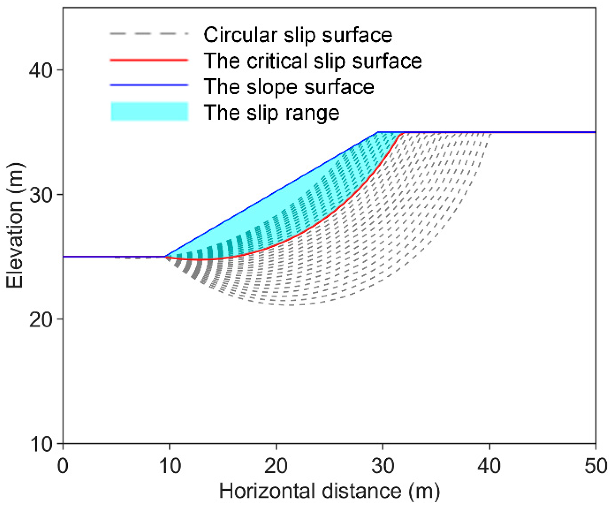
2.2. Critical Slip Surface Determination Incorporated with the Monte Carlo Method

In debris-flow source areas, the soils are typically inhomogeneous and have significant spatial variability in strength parameters, which increases the difficulty of critical slip surface searching. In this case, the critical source slip surface is usually of the compound fold type, and the Swedish method is no longer applicable. To determine the location and depth of the slip surface and to calculate the volume of the initiation source for the debris flow hazard, the Monte Carlo method is used to simulate the spatial distribution of the compound folded surface and the spatial uncertainty of soil parameters. The Monte Carlo method is a repeated random sampling method that has been applied to debris flow studies, and we have conducted a bed-sediment entrainment assessment study using this method [37]. In this paper, the method for searching the critical slip surface and calculating the initiation source volume can be summarized as follows.
(1)
Composite critical slip surface determination.
Initially, the soil parameters are assumed to be uniformly distributed across the study area, and the Swedish circular method is used to identify the circular slip surface corresponding to the minimum factor. Then, the range limits of the shear inlet and outlet points of the trial surface are defined according to the circular surface. Based on the defined range limits of the shear inlet and outlet points, a specific search domain is delineated around the circular critical surface. The number of Monte Carlo simulation steps is specified. In each step, a composite slip surface is randomly generated within the defined boundaries using the slice sub-nodes as feature points. The generated composite slip surface should meet the following geometric adequacy requirements [38].
  • The slip surface should be located entirely within the slope body range, and the shear inlet and shear outlet are on the slope surface;
  • There should be smooth transitions between adjacent slip slice segments and no sharp corners. The angle between two adjacent slip slice segments should be greater than 90°;
  • The horizontal spacing of adjacent nodes should be greater than the minimum horizontal spacing to avoid overlap of the slice division nodes.
The search domain determined by the critical circular surface and the above geometric adequacy requirements ensure that all generated trail slip surfaces are valid for the determination of slope stability. Calculate the stability factor of each generated slip surface to determine the slip surface stability. When the simulation steps are sufficient, the generated slip surface corresponding to the minimum stability factor is the critical slip surface { c | ( x o , z o ) , ( x 1 , z 1 ) , , ( x n , z n ) } . Given the average width of the source area gully w , the initiation source volume can be calculated as:
V = 1 2 i = 1 n w [ s ( x i ) + s ( x i 1 ) z i z i 1 ] ( x i x i 1 )
(2)
Considering the spatial variability of the soil, calculate the range of the critical slip surface and the initiation source volume.
Define the input soil parameters that are sensitive in terms of source initiation. These parameters are assumed to follow the normal distribution. Then, create a dataset for each parameter, which should be sufficient to cover the spatial uncertainties of the soil properties. Specify the number of Monte Carlo simulation steps, and a kind of soil parameter spatial distribution is generated in each step based on the dataset. As for each generated spatial distribution of soil parameters, the method described in (1) is applied to search the corresponding critical slip surface and estimate the initiation source volume. Eventually, the range of the critical slip surface and the initiation source volume resulting from the spatial variability of soil properties can be assessed.

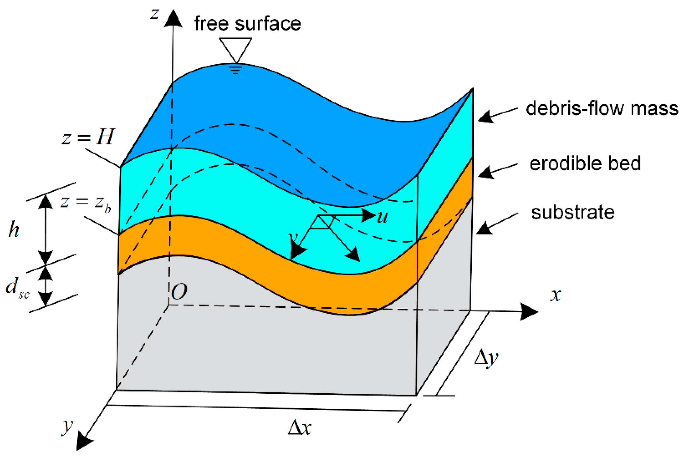
3. Entrainment-Incorporated Numerical Model

In our prior study [24], we developed a dynamic model for debris flow process simulation that incorporated the bed-entrainment estimation method based on momentum conservation. The schematic diagram of the dynamic model is shown in Figure 4.
The mass conservation equation, also known as the continuity equation, is
h t + ( u h ) x + ( v h ) y = E
The momentum conservation equations in both x and y directions are expressed below:
( u h ) t + ( u 2 h ) x + ( u v h ) y = H x g h + μ k ρ [ 2 ( u h ) x 2 + 2 ( u h ) y 2 ] τ x ρ
( v h ) t + ( u v h ) x + ( v 2 h ) y = H y g h + μ k ρ [ 2 ( v h ) x 2 + 2 ( v h ) y 2 ] τ y ρ
where h represents the thickness of the flow mass; u and v denote the velocity of the flow in horizontal x and y directions, respectively; t signifies the computational time; H = z b + h corresponds to the height of the free surface relative to the channel bed; E = d s c / t is indicative of the time-dependent entrainment rate on the bed sediment; z b denotes the height of the bed surface; g refers to the gravitational acceleration; μ is the dynamic viscosity coefficient of the flow mass; k is the earth pressure coefficient, which is the ratio of the vertical normal stress to the horizontal one; ρ represents the density of the flow mass.
Equations (6) and (7) feature τ x and τ y , which contribute to the dissipation of energy during the debris flow propagation. Notably, we utilize the Voellmy rheological constitutive model in contrast to our prior work, as it is better suited for long-distance debris flow simulation compared to the viscous and Coulomb friction model [39]. The Voellmy model includes two distinct components, i.e., a basal friction term that characterizes the stopping mechanism and a turbulent term that captures the velocity-dependent energy losses.
τ x = s i g n ( u ) u 2 + v 2 ( ρ g h c o s θ x t a n φ v o e l l m y + ρ g u 2 + v 2 C z 2 )
τ y = s i g n ( v ) u 2 + v 2 ( ρ g h c o s θ y t a n φ v o e l l m y + ρ g u 2 + v 2 C z 2 )
where θ x and θ y are the bed surface slope angles along x and y directions, respectively; φ v o e l l m y represents the internal friction angle of debris flow; C z is the Chezy coefficient; s i g n ( ) denotes the symbolic function in mathematics.
The bed-sediment entrainment plays a crucial role in the expansion of debris-flow mass volume and run-out extent [40,41]. To estimate the bed-sediment entrainment along the path, we incorporate a physically based dynamic method based on momentum conservation into our debris-flow numerical model [24]. The entrainment that occurs during debris flow propagation can be quantitatively described by the erosion rate, which is given by
E = g h c o s θ [ t a n φ d ( 1 λ d ) t a n φ b e d ] ( 1 s 1 ) v 1 ¯  
where φ d is the bulk basal friction angle of the flow mass, as introduced by Hungr and McDougall [42]; λ d is the pore-pressure coefficient of the erodible bed; s 1 is the fitting parameter related to the vertical velocity profile ranging from 0 to 1 ; v 1 ¯ is the mean velocity through the depth.
The explicit finite difference method on staggered Eulerian grids was utilized to numerically solve the governing equations, which has been elaborated on in our prior work [24]. The staggered grid arrangement entails that the depth of the debris flow mass resides at the center of each cell, whereas the velocities in both directions are located at the center of each cell’s edge. To discretize space, we employed the central difference scheme, while the semi-Lagrangian method is used for time advance. Moreover, we applied the Courant–Friedrichs–Lewy condition to enforce stability constraints on explicit difference schemes and process the half-step calculation data [43].

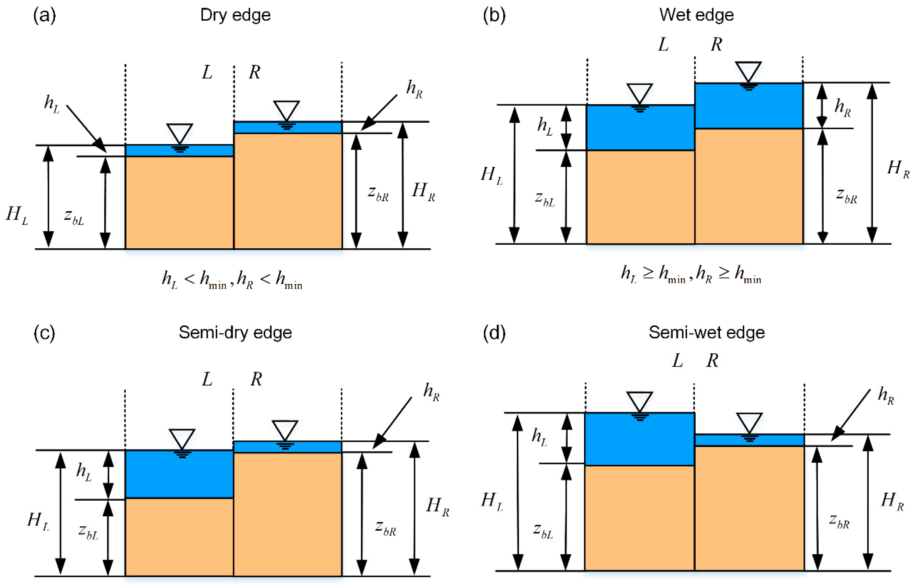
4. Wet/Dry Front Treatment over Complex Topography

To enhance our debris-flow numerical model’s capacity for simulating dynamic processes, we propose an improved wet/dry front treatment method that can be utilized with the FDM scheme. Inspired by a previously developed approach [32,44] that was exclusively adaptive to unstructured grids in the FVM scheme, we have modified and extended the method to accommodate rectangular grids in the FDM scheme, thereby improving both computational stability and accuracy.
The proposed method defines a set of rules for calculating wet/dry cells based on their wet/dry conditions, as well as inflow/outflow conditions in the velocity-dependent direction. A minimum depth denoted as h m i n , is pre-defined as the fundamental threshold for the categorization of wet/dry grid cell types. The proposed wet/dry front treatment method consists of three major steps, which are summarized as follows.
Step 1: the classification of wet/dry cell edges. Divide the edges of all computation domain cells into four categories based on the depth and surface level of the neighboring cells, as illustrated in Figure 5.
  • Dry edge. The flow depths of both neighboring cells are smaller than h m i n , which is mathematically expressed as h L < h m i n ,   h R < h m i n , as shown in Figure 5a.
  • Wet edge: in contrast to the dry edge, the flow depths of both neighboring cells are greater than h m i n , which is h L h m i n ,     h R h m i n , as shown in Figure 5b.
  • Semi-dry edge: the flow depth of one neighboring cell is greater than h m i n while the other one is less than h m i n , and the flow surface level of the dry side is higher than that of the wet side. For example, h L h m i n ,   h R < h m i n , and H L H R , as shown in Figure 5c;
  • Semi-wet edge: the flow depth condition of the cells on both sides is the same as that of the semi-dry edge, but the flow surface level of the wet side is higher than that of the dry side—for example, h L > h m i n ,   h R h m i n , and H L > H R , as shown in Figure 5d.
Figure 5. Four types of cell edge delineation.
Water 15 01592 g005
In our treatment approach, we temporarily define both the dry and semi-dry edges as closed boundaries. This implies that the corresponding flow velocity should be zero to ensure that there is no flow mass passing through these boundaries.
Step 2: Wet/dry condition determination. Based on the four types of cell edges recognized in Step 1, the wet/dry condition of all computational domain cells is further determined with respect to the cell depth and surface level.
Wet cell. Including two kinds of cells, i.e., first, the flow depth is greater than a submergence depth h w e t which is commonly suggested as 2.5 h m i n by Xia et al. [45]. Second, the flow depth is less than h w e t , and all four surrounding cells have wet or semi-wet edges.
Invalid dry cell: the flow depth of the cell is less than h m i n , and all the surrounding four cells have edges belonging to dry or semi-dry edges.
Effective dry cell: the cells belong to neither of the above types.
Step 3: updating the flow depth and velocities of a cell. The determined wet/dry cells are calculated in the following numerical schemes. The criteria are listed below. Wet cells normally participate in the iterative calculation of the momentum and continuity equations. Effective dry cells only update the flow depth and flow surface level through the continuity equation unless their net flux directs to the wet region. The invalid dry cells are temporarily removed from the current computation domain, with the velocities along both directions set to zero, while the depth reserves in this time step.
The above procedures are performed at each iteration time step. The wet/dry conditions of the cells are continuously updated based on the flow depth and topography at each time step. Any mass outflow from a dry cell is prohibited, and the dry cell will not be re-included in the calculation until sufficient mass is available to flow through it. At each time step, the calculation of all invalid dry cells is omitted, resulting in a significant improvement in computational efficiency.

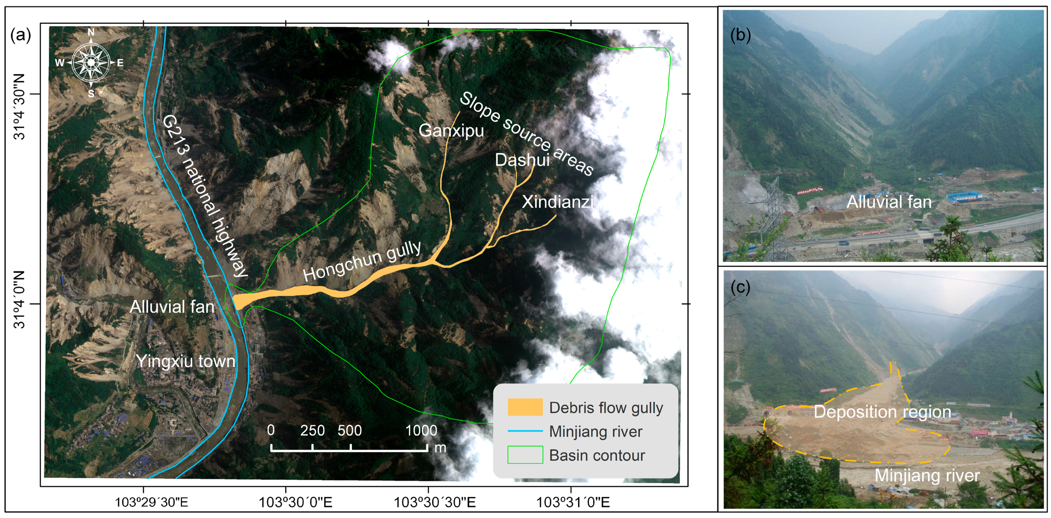
5. Case Study: The 2010 Hongchun Debris-Flow Event in the Yingxiu Town, China

This section presents a case study that aims to validate the proposed method’s effectiveness in simulating actual debris-flow events, using the 2010 Hongchun debris-flow event as an example. First, the critical slip surface range and the initiation source volume are estimated through the application of the Monte Carlo simulation and limit equilibrium method. Subsequently, the proposed entrainment-incorporated numerical model with the wet/dry front treatment is utilized to simulate the wetting and drying process over complex terrain.

5.1. The Overview of the 2010 Hongchun Debris-Flow Event

The Hongchun catchment spans an area of 5.90   km 2 and is situated on the left bank of the Minjiang river, to the northeast of Yingxiu Town. The catchment is adjacent to the epicenter of the 2008 Wenchuan earthquake. Notably, the incised V-shaped gully in the area, illustrated in Figure 6a, has a longitudinal length of 3.6   km and an elevation range of 880 to 1700   m . The gully’s slope gradient averages 35.8   % . Following the 2008   Ms .8.0 Wenchuan earthquake, a reported 350 × 10 m 3 volume of loose material was present, causing severe channel blockages and becoming a potential source of subsequent debris flows within the catchment.
The occurrence of the debris-flow event was due to severe rainfall falling between 12 and 14 August 2010, which resulted in a total of 162.1 mm of precipitation recorded in the catchment. Xu et al. [46] and Shen et al. [47] indicated that the event was triggered when the rainfall intensity reached 16.4   mm / h . Three major potential sources at the branch gullies of Ganxipu, Dashui, and Xindianzi were reported, with initial mass volumes of 11.2 × 10 4   m 3 , 3.9 × 10 4   m 3 , and 3.2 × 10 4   m 3 , respectively. A total of 80.5 × 10 4   m 3 of erodible bed material was observed, which was identified as a potential component of the overriding debris-flow mass. Finally, approximately 40.0 × 10 4   m 3 of the total mass was deposited in the Minjiang River [25].

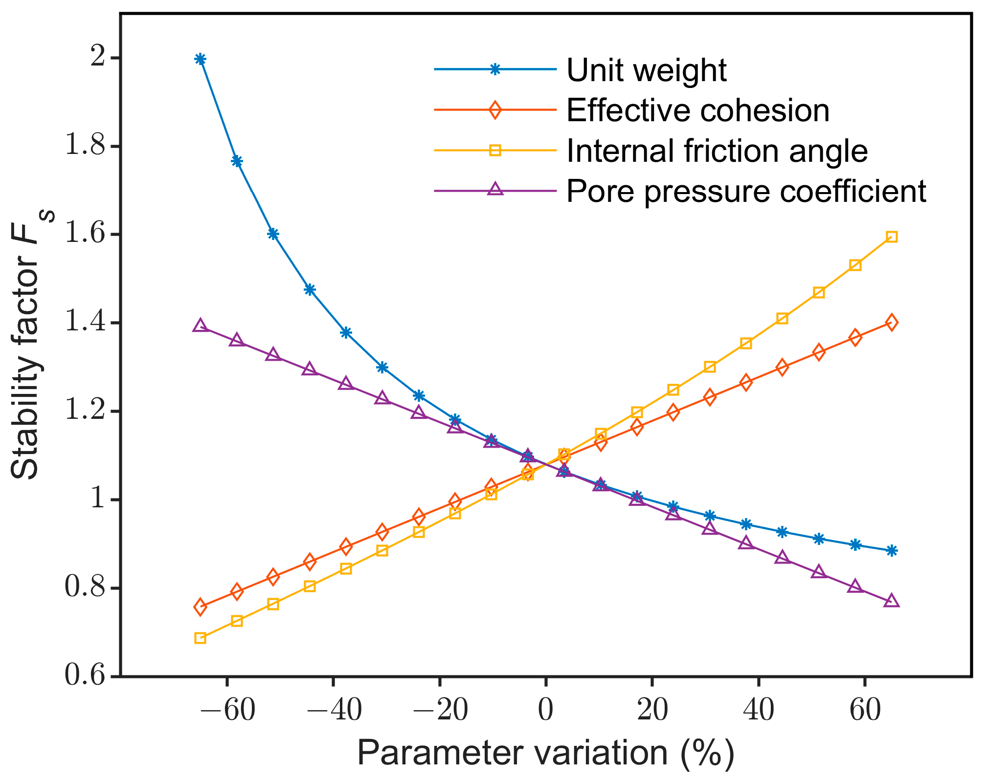
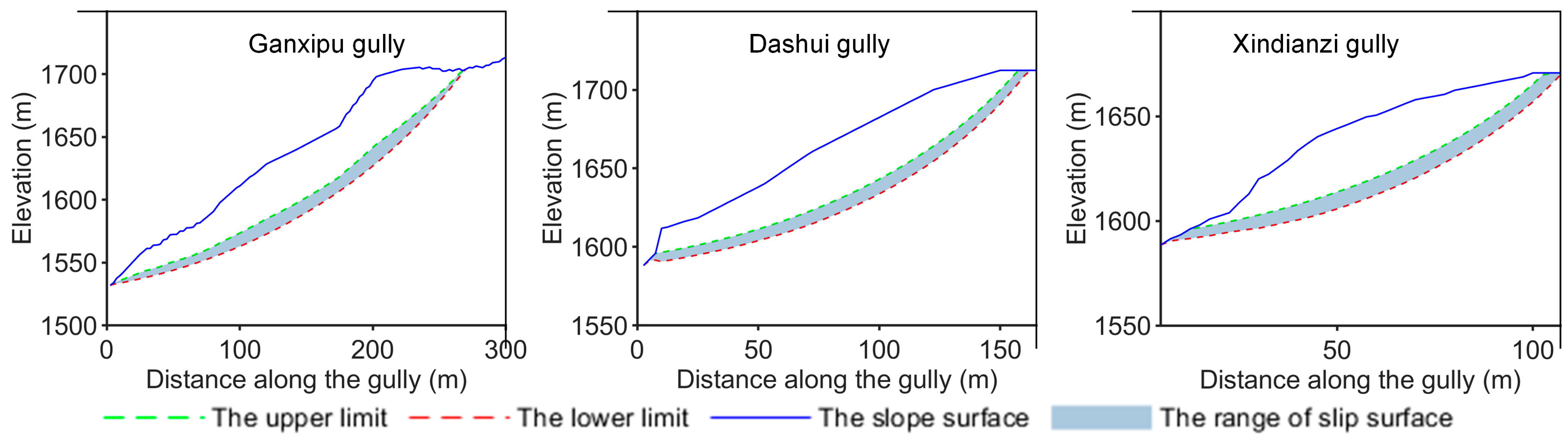
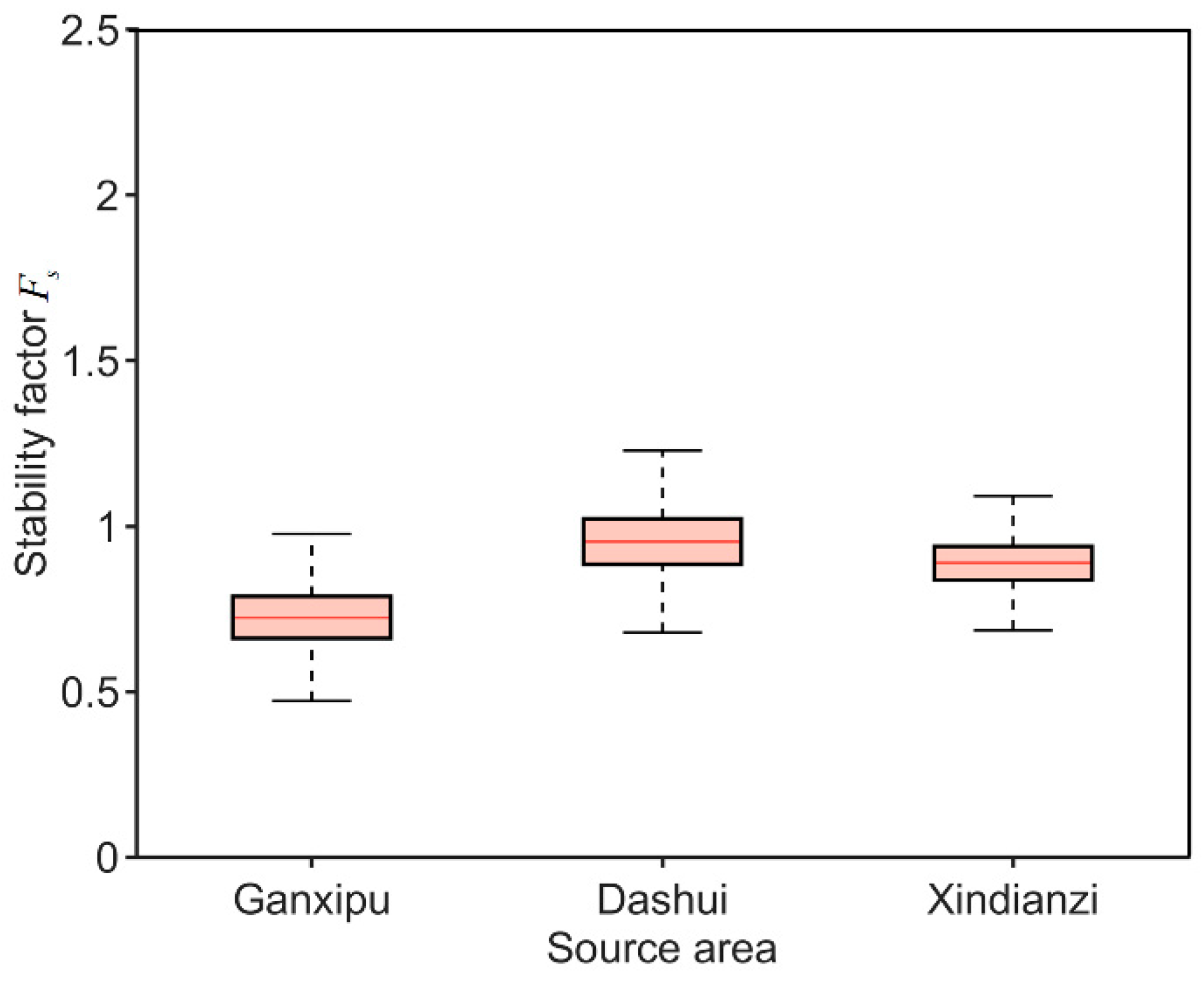
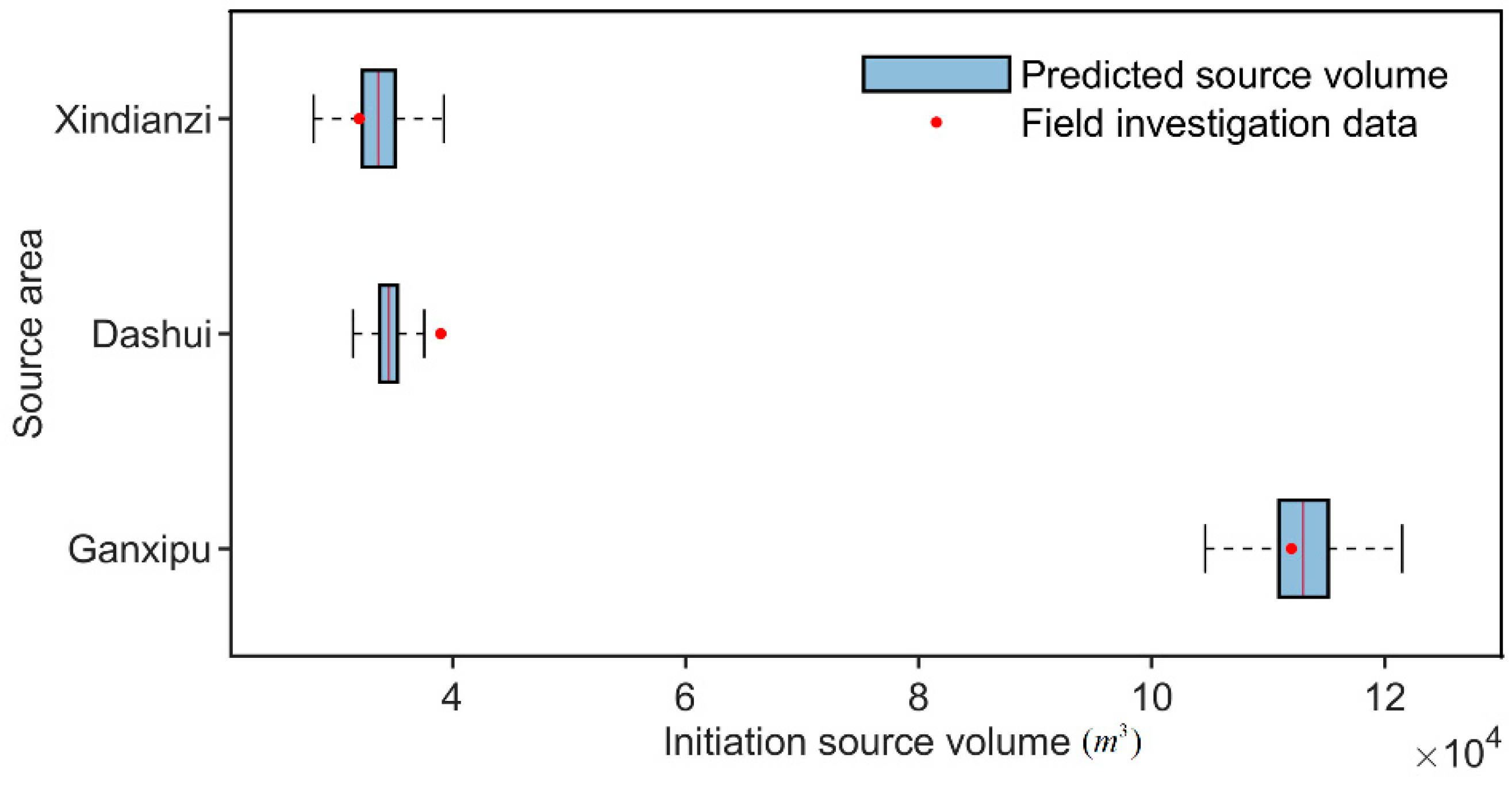
5.2. The Physically Based Estimation of the Slope Initiation Source

In this study, 2.5   m resolution DTM (Digital Terrain Model) data, consisting of 1424 rows and 1817 columns cells in total, are employed for the slope initiation source estimation and the subsequent dynamic process simulation. This DTM data are generated based on the resampling of the modified high-resolution grid data in Ouyang et al. [25]. Although the pre-event topography of the entire catchment is not available, the post-event topography is partially replaced by the pre-event data of the downstream alluvial fan. Moreover, we reconstruct and adjust the elevation data in three source areas (Ganxipu, Dashui, and Xindianzi) according to the pre-earthquake contour lines and debris-flow survey reports.
Except for the erosion source located in the middle of the main gully, three major potential sources at the branch gullies of Ganxipu, Dashui, and Xindianzi (Figure 6a) contributed most of the initiation source mass. We take the average elevation along the vertical gully direction for slope stability analysis in these three source areas, respectively. According to the survey data, the average width of the upstream Ganxipu gully is about 12.0   m , while the width of the Dashui gully and Xindianzi gully ranges from 6.0   to   10.0   m and 12.0   to   20.0   m , respectively. The unit weight of soil in the source area is consistent with the debris flow, with an average value of 20.2   kN / m 3 . Several geotechnical tests on the sediment of the gullies were conducted to reveal the soil parameters. The calculated internal friction angle is 28.0° and the effective cohesion is 2.9   kPa . To cover the spatial uncertainty of the soil parameters, we set the coefficient of variation and parameter ranges shown in Table 1.
A total of 10,000 Monte Carlo simulation tracks are implemented using the method proposed in this paper. Each simulation generates a spatial distribution of soil strength parameters. The corresponding critical slip surface is obtained. Figure 7 shows the distribution of all possible critical slip surfaces for each source area generated by the Monte Carlo simulation. As expected, the slip surfaces in each source area are roughly in the form of compound folds and are presented in the reasonable spatial range. The area enclosed by the upper and lower limits of the slip surface (Figure 7) represents the predicted minimum and maximum initiation source profiles, respectively.
The Monte Carlo simulation also generates valid distributions of the predicted initiation source volume and stability factors of the critical slip surface in all source regions. The stability factors in all three areas are mostly in the range of 0.5 to 0.9 (Figure 8), which indicates the serious instability of the slope soil. Combined with the average width of the three branch gullies, the initiation source volume range of the three areas is shown in Figure 9. The median values of the predicted source volume in the three areas are 11.29 × 10 4   m 3 , 3.45 × 10 4   m 3 , and 3.38 × 10 4   m 3 , respectively. Compared with the corresponding survey data, the predicted errors of the initiation source volume in the three potential source areas are 0.09 × 10 4   m 3 , 0.45 × 10 4   m 3 , and 0.18 × 10 4   m 3 , which are all within an acceptable range.

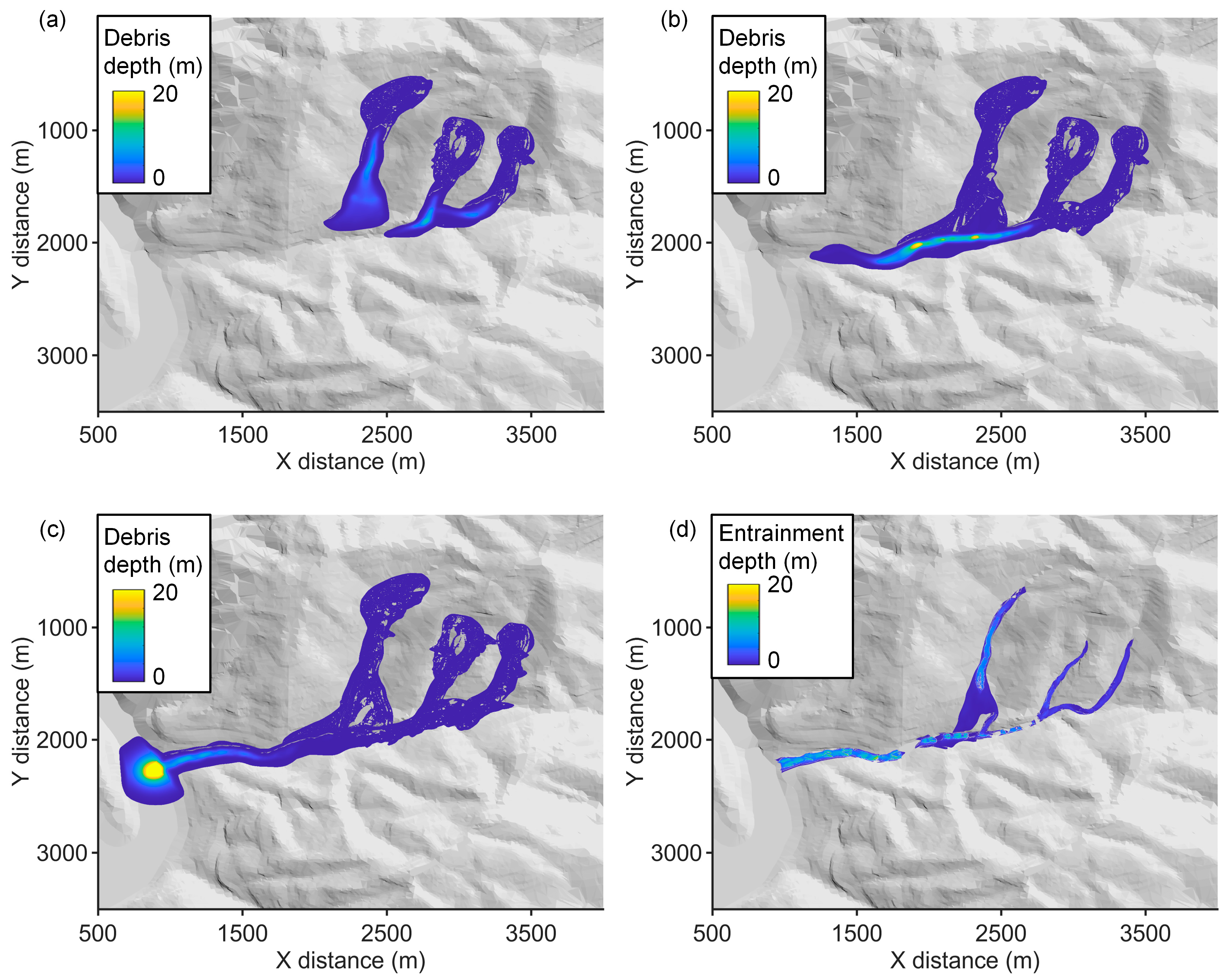
5.3. Numerical Simulation of the Debris-Flow Dynamic Process

To simulate the wetting and drying process of the observed debris flow event, we use the predicted initiation source as the initial source in the three source areas. The average surface of the predicted range of the critical slip surface is used to determine the location and depth of the initial source along the gully. The simulation is conducted on the DTM data described in Section 5.2, and the 2.5 × 2.5   m terrain cells are used as difference grids. Table 2 presents the parameter values employed in the simulation.
The simulated flow-depth distribution of the event at various time intervals is depicted in Figure 10a–c. The wet/dry fronts of debris flow first propagate through the three branch gullies before converging in the middle and upper sections of the main gully at the moment of 50   s . Subsequently, the confluence wet/dry fronts propagate along the main gully, producing obvious bed-sediment entrainment (shown in Figure 10d), and deposits downstream, eventually.
According to our predictions, the total flow mass involved in the debris-flow event is 92.73 × 10 4   m 3 , of which 48.32 × 10 4   m 3 rushes out, and over half is deposited at the Minjiang river. The predicted results for the flow mass involved in the process and deposited at the Minjiang river are consistent with the field survey data, where the total volume is 80.5 × 10 4   m 3 and the volume deposited at the Minjiang river is 40.5 × 10 4   m 3 [25]. The maximum deposition depth is 22.45   m , located at the downstream alluvial fan. Additionally, the middle and lower sections of the main gully show the most significant entrainment, with a maximum erosion depth of 17.75   m (Figure 10d). The predicted deposition and accumulative erosion depth are relatively close to the in situ survey data, in which the maximum deposition depth of more than 20.0   m and the maximum erosion depth of almost 20.0   m have been reported [25,48]. Therefore, the depth and entrainment distribution of the debris flow are in good agreement with the in situ survey. These results indicate that the proposed methods in this paper reproduce the actual debris-flow event well by utilizing the Monte Carlo method for predicting the initiation source and employing wet/dry front treatment integrated into the entrainment-incorporated model.

6. Discussion

In this paper, we present an integrated approach to simulating debris flow dynamics that includes the physically based estimation of slope initiation sources and the numerical simulation of dynamic processes. The 2010 Hongchun debris-flow event is used as a case study to verify the effectiveness and performance of the method.

6.1. Advantages

The paper presents a slope source estimation method that utilizes unsaturated soil mechanics and limit equilibrium theory. Unlike conventional methods that simulate debris flow initiation by using predefined flow curves or artificially defining a source thickness, the proposed method considers the mechanism of slope source initiation and avoids subjective source definition. The spatial variability of soil parameters can be simulated by the Monte Carlo method to obtain the range of possible critical slip fracture surfaces and the interval of the initiation source. In the proposed wet/dry treatment method, all dry cells are temporarily removed from the computational domain at each time step, which improves computational efficiency. The method is integrated into the debris-flow numerical model, which enhances the stability of the numerical scheme and improves the prediction accuracy of wet/dry front propagation.

6.2. Limitations and Future Works

The slope source initiation model faces challenges when searching for the critical slip surface accurately and efficiently due to the presence of rock fissures in the soil and the error of set parameters, despite the pre-defined search domain. To overcome this challenge, future research could combine heuristic algorithms to find the global minimum stability factor. Moreover, the soil variability is not only noticeable in soil stratifications, such as soft interlayers, but is also influenced by time-dependent effects such as creep or consolidation, making it important to consider soil stratifications and time-dependent variability synthetically in future studies for a more precise estimation of the source initiation range. Regarding the case study of the Hongchun debris-flow event, while the topography data in the alluvial fan and source areas have been replaced and reconstructed based on partial pre-event data and contour lines, respectively, this modification to the DTM data may pose difficulties in comparing the predicted slip surface with the actual landslides triggering the debris-flow event. Therefore, it is crucial to discuss the impact of such modifications on source initiation estimation and dynamic process simulation for further work. In future studies, every possible effort should be made to obtain accurate and timely topographic data of actual debris-flow events; thus, more case studies and specific comparisons should be carried out to improve the prediction of the slope source initiation and the dynamic process of debris flows.
This paper presents an integrated method for studying the dynamic processes of debris flows, which can serve as a valuable reference for disaster prevention and control. To further advance the integration of numerical simulation with disaster prevention, a promising approach is to investigate the coupling effect between debris flows and damaged structures, based on the theory of structural dynamics [49], with the aim of analyzing the damage mechanisms of affected structures [50]. Additionally, future research could explore the combination of numerical simulation results with geographical scenarios [51] to enhance public awareness of debris flow disasters [52] and ultimately reduce their impact. Such efforts would help to mitigate the devastating effects of debris flows and contribute to the advancement of disaster prevention and control strategies.

7. Conclusions

In this paper, we propose an integration method for simulating debris-flow dynamics, including the physically based slope initiation source estimation and dynamic process simulation with the entrainment-incorporated model. In the proposed initiation source estimated method, the location and depth of the composite folding slip surface are considered random variables in searching for the critical slip surface corresponding to the minimum stability factor. Considering the spatial variability of soil parameters, a sufficiently large dataset of input parameters obeying a normal distribution is included in the simulation to obtain the range of critical slip surfaces and initiation source volumes. In our debris-flow numerical model, we incorporate a dynamic method in order to estimate the entrainment rate. Moreover, we propose a wet/dry front treatment aiming at enhancing computational stability and accuracy. In combination with the wet/dry types and inflow/outflow conditions at cell edges, the cells of the computational domain are analyzed and calculated separately to capture wet/dry fronts.
The 2010 Hongchun debris-flow event is used as a case study to test the effectiveness of the initiation source estimated method and the performance of the real debris-flow process simulation. Slope stability analysis and Monte Carlo simulation are carried out in three initial source areas of Ganxipu, Dashui, and Xindianzi to estimate the critical slip surface. The spatial variability of soil parameters generates the range of the critical slip surface and initiation source volume, which is close to the data obtained from field investigation. The numerical model is applied to simulate the complex dynamic process based on the predicted initiation source. The results including the erosion and deposition volume on the alluvial fan are close to the survey data.
While the proposed integrated method shows promise, it is limited in finding the global minimum stability factor efficiently, and there is a lack of complete pre-event topography data. Future research should aim to address these limitations in order to estimate the slope source initiation more precisely and better reproduce the dynamic process of debris flows.

Author Contributions

Z.H. led the research program. M.Z., C.L. and Y.M. designed the simulation. Z.H. and M.L. wrote the manuscript. Y.L., W.X. and H.D. reviewed and edited the manuscript. All authors have read and agreed to the published version of the manuscript.

Funding

This research was funded by the National Natural Science Foundation of China (Grant No. 52078493); the Natural Science Foundation of Hunan Province (Grant No. 2022JJ30700); the Natural Science Foundation for Excellent Young Scholars of Hunan (Grant No. 2021JJ20057); the Innovation Provincial Program of Hunan Province (Grant No. 2020RC3002); and the Training Program for Excellent Young Innovators of Changsha (No. kq2106018).

Data Availability Statement

The data used in this study are available on request from the corresponding author.

Conflicts of Interest

The authors declare no conflict of interest.

References

  1. Pudasaini, S.P. A general two-phase debris flow model. J. Geophys. Res. Earth Surf. 2012, 117, F03010. [Google Scholar] [CrossRef]
  2. Dowling, C.A.; Santi, P.M. Debris flows and their toll on human life: A global analysis of debris-flow fatalities from 1950 to 2011. Nat. Hazards 2014, 71, 203–227. [Google Scholar] [CrossRef]
  3. Han, Z.; Ma, Y.; Li, Y.; Zhang, H.; Chen, N.; Hu, G.; Chen, G. Hydrodynamic and topography based cellular automaton model for simulating debris flow run-out extent and entrainment behavior. Water Res. 2021, 193, 116872. [Google Scholar] [CrossRef] [PubMed]
  4. Scheidl, C.; Rickenmann, D. Empirical prediction of debris-flow mobility and deposition on fans. Earth Surf. Process. Landforms 2010, 35, 157–173. [Google Scholar] [CrossRef]
  5. Du, J.; Fan, Z.J.; Xu, W.T.; Dong, L.Y. Research progress of initial mechanism on debris flow and related discrimination methods: A review. Front. Earth Sci. 2021, 9, 629567. [Google Scholar] [CrossRef]
  6. Liu, X.; Wang, F.; Nawnit, K.; Lv, X.; Wang, S. Experimental study on debris flow initiation. Bull. Eng. Geol. Environ. 2020, 79, 1565–1580. [Google Scholar] [CrossRef]
  7. Tang, H.; McGuire, L.A.; Rengers, F.K.; Kean, J.W.; Staley, D.M.; Smith, J.B. Evolution of debris-flow initiation mechanisms and sediment sources during a sequence of postwildfire rainstorms. J. Geophys. Res. Earth Surf. 2019, 124, 1572–1595. [Google Scholar] [CrossRef]
  8. Chen, H.X.; Zhang, L.M.; Zhang, S.; Xiang, B.; Wang, X.F. Hybrid simulation of the initiation and runout characteristics of a catastrophic debris flow. J. Mt. Sci. 2013, 10, 219–232. [Google Scholar] [CrossRef]
  9. Zhong, W.; He, N.; Cosgrove, T.; Zhu, Y.J.; Fu, L. Analysis of the correlation between fractal dimension of gravelly soil and debris-flow initiation through in-situ experiments. Appl. Ecol. Environ. Res. 2019, 17, 7573–7589. [Google Scholar] [CrossRef]
  10. Zhou, J.W.; Cui, P.; Yang, X.G. Dynamic process analysis for the initiation and movement of the Donghekou landslide-debris flow triggered by the Wenchuan earthquake. J. Asian Earth Sci. 2013, 76, 70–84. [Google Scholar] [CrossRef]
  11. Hu, M.J.; Wang, R.; Chen, Z.X.; Wang, Z.B. Initiation process simulation of debris deposit based on particle flow code. Rock Soil Mech. 2010, 31, 394–397. (In Chinese) [Google Scholar]
  12. Liu, J.; Nakatani, K.; Mizuyama, T. Effect assessment of debris flow mitigation works based on numerical simulation by using Kanako 2D. Landslides 2013, 10, 161–173. [Google Scholar] [CrossRef]
  13. Lin, D.G.; Hsu, S.Y.; Chang, K.T. Numerical simulations of flow motion and deposition characteristics of granular debris flows. Nat. Hazards 2009, 50, 623–650. [Google Scholar] [CrossRef]
  14. Wang, C.; Li, S.; Esaki, T. GIS-based two-dimensional numerical simulation of rainfall-induced debris flow. NHESS 2008, 8, 47–58. [Google Scholar] [CrossRef]
  15. Luna, B.Q.; Remaître, A.; Van Asch, T.W.; Malet, J.P.; Van Westen, C.J. Analysis of debris flow behavior with a one dimensional run-out model incorporating entrainment. Eng. Geol. 2012, 128, 63–75. [Google Scholar] [CrossRef]
  16. Cannon, S.H.; Gartner, J.E.; Wilson, R.C.; Bowers, J.C.; Laber, J.L. Storm rainfall conditions for floods and debris flows from recently burned areas in southwestern Colorado and southern California. Geomorph 2008, 96, 250–269. [Google Scholar] [CrossRef]
  17. Zhou, J.; Li, E.; Yang, S.; Wang, M.; Shi, X.; Yao, S.; Mitri, H.S. Slope stability prediction for circular mode failure using gradient boosting machine approach based on an updated database of case histories. Saf. Sci. 2019, 118, 505–518. [Google Scholar] [CrossRef]
  18. Hazari, S.; Sharma, R.P.; Ghosh, S. Swedish circle method for pseudo-dynamic analysis of slope considering circular failure mechanism. Geotech. Geol. Eng. 2020, 38, 2573–2589. [Google Scholar] [CrossRef]
  19. Yang, Y.; Wu, W.; Zheng, H. Searching for critical slip surfaces of slopes using stress fields by numerical manifold method. JRMGE 2020, 12, 1313–1325. [Google Scholar] [CrossRef]
  20. Liu, X.; Li, D.Q.; Cao, Z.J.; Wang, Y. Adaptive Monte Carlo simulation method for system reliability analysis of slope stability based on limit equilibrium methods. Eng. Geol. 2020, 264, 105384. [Google Scholar] [CrossRef]
  21. Crosta, G.B.; Imposimato, S.; Roddeman, D. Numerical modeling of 2-D granular step collapse on erodible and nonerodible surface. J. Geophys. Res. Earth Surf. 2009, 114, F03020. [Google Scholar] [CrossRef]
  22. Horton, P.; Jaboyedoff, M.; Rudaz, B.E.A.; Zimmermann, M. Flow-R, a model for susceptibility mapping of debris flows and other gravitational hazards at a regional scale. Nat. Hazards Earth Syst. Sci. 2013, 13, 869–885. [Google Scholar] [CrossRef]
  23. Iverson, R.M.; George, D.L. A depth-averaged debris-flow model that includes the effects of evolving dilatancy. I. Proc. R. Soc. A 2014, 470, 20130819. [Google Scholar] [CrossRef]
  24. Han, Z.; Chen, G.; Li, Y.; Tang, C.; Xu, L.; He, Y.; Wang, W. Numerical simulation of debris-flow behavior incorporating a dynamic method for estimating the entrainment. Eng. Geol. 2015, 190, 52–64. [Google Scholar] [CrossRef]
  25. Ouyang, C.; He, S.; Tang, C. Numerical analysis of dynamics of debris flow over erodible beds in Wenchuan earthquake-induced area. Eng. Geol. 2015, 194, 62–72. [Google Scholar] [CrossRef]
  26. Armanini, A.; Fraccarollo, L.; Rosatti, G. Two-dimensional simulation of debris flows in erodible channels. Comput. Geosci. 2009, 35, 993–1006. [Google Scholar] [CrossRef]
  27. Castro-Orgaz, O.; Chanson, H. Ritter’s dry-bed dam-break flows: Positive and negative wave dynamics. Environ. Fluid Mech. 2017, 17, 665–694. [Google Scholar] [CrossRef]
  28. Chen, C.; Qi, J.; Li, C.; Beardsley, R.C.; Lin, H.; Walker, R.; Gates, K. Complexity of the flooding/drying process in an estuarine tidal-creek salt-marsh system: An application of FVCOM. J. Geophys. Res. Ocean. 2008, 113, C07052. [Google Scholar] [CrossRef]
  29. Liang, D.; Lin, B.; Falconer, R.A. A boundary-fitted numerical model for flood routing with shock-capturing capability. J. Hydrol. 2007, 332, 477–486. [Google Scholar] [CrossRef]
  30. Medeiros, S.C.; Hagen, S.C. Review of wetting and drying algorithms for numerical tidal flow models. Int. J. Numer. Meth. Fluids 2013, 71, 473–487. [Google Scholar] [CrossRef]
  31. Liu, D.; Tang, J.; Wang, H.; Cao, Y.; Bazai, N.A.; Chen, H.; Liu, D. A new method for wet-dry front treatment in outburst flood simulation. Water 2021, 13, 221. [Google Scholar] [CrossRef]
  32. Huang, Y.; Zhang, N.; Pei, Y. Well-balanced finite volume scheme for shallow water flooding and drying over arbitrary topography. Eng. Appl. Comput. Fluid Mech. 2013, 7, 40–54. [Google Scholar] [CrossRef]
  33. Le, H.A.; Lambrechts, J.; Ortleb, S.; Gratiot, N.; Deleersnijder, E.; Soares-Frazão, S. An implicit wetting–drying algorithm for the discontinuous Galerkin method: Application to the Tonle Sap, Mekong River Basin. Environ. Fluid Mech. 2020, 20, 923–951. [Google Scholar] [CrossRef]
  34. Costabile, P.; Macchione, F. Enhancing river model set-up for 2-D dynamic flood modelling. Environ. Model. Softw. 2015, 67, 89–107. [Google Scholar] [CrossRef]
  35. Baeza, A.; Donat, R.; Martinez-Gavara, A. A numerical treatment of wet/dry zones in well-balanced hybrid schemes for shallow water flow. Appl. Numer. Math. 2012, 62, 264–277. [Google Scholar] [CrossRef]
  36. Zhou, X.P.; Cheng, H. Stability analysis of three-dimensional seismic landslides using the rigorous limit equilibrium method. Eng. Geol. 2014, 174, 87–102. [Google Scholar] [CrossRef]
  37. Han, Z.; Chen, G.; Li, Y.; He, Y. Assessing entrainment of bed material in a debris-flow event: A theoretical approach incorporating Monte Carlo method. ESPL 2015, 40, 1877–1890. [Google Scholar] [CrossRef]
  38. Zhang, L.Y.; Zhang, J.M. Extended algorithm using Monte Carlo techniques for searching general critical slip surface in slope stability analysis. Yantu Gongcheng Xuebao (Chin. J. Geotech. Eng.) 2006, 28, 857–862. (In Chinese) [Google Scholar] [CrossRef]
  39. Naef, D.; Rickenmann, D.; Rutschmann, P.; McArdell, B.W. Comparison of flow resistance relations for debris flows using a one-dimensional finite element simulation model. NHESS 2006, 6, 155–165. [Google Scholar] [CrossRef]
  40. Han, Z.; Su, B.; Li, Y.; Dou, J.; Wang, W.; Zhao, L. Modeling the progressive entrainment of bed sediment by viscous debris flows using the three-dimensional SC-HBP-SPH method. Water Res. 2020, 182, 116031. [Google Scholar] [CrossRef]
  41. Iverson, R.M.; Reid, M.E.; Logan, M.; LaHusen, R.G.; Godt, J.W.; Griswold, J.P. Positive feedback and momentum growth during debris-flow entrainment of wet bed sediment. Nat. Geosci. 2011, 4, 116–121. [Google Scholar] [CrossRef]
  42. Hungr, O.; McDougall, S. Two numerical models for landslide dynamic analysis. Comput. Geosci. 2009, 35, 978–992. [Google Scholar] [CrossRef]
  43. Bingham, H.B.; Zhang, H. On the accuracy of finite-difference solutions for nonlinear water waves. J. Eng. Math. 2007, 58, 211–228. [Google Scholar] [CrossRef]
  44. Zhao, D.H.; Shen, H.W.; Tabios, G.Q., III; Lai, J.S.; Tan, W.Y. Finite-volume two-dimensional unsteady-flow model for river basins. J. Hydraul. Eng. 1994, 120, 863–883. [Google Scholar] [CrossRef]
  45. Xia, J.; Falconer, R.A.; Lin, B.; Tan, G. Modelling flood routing on initially dry beds with the refined treatment of wetting and drying. IJRBM 2010, 8, 225–243. [Google Scholar] [CrossRef]
  46. Xu, Q.; Zhang, S.; Li, W.L.; Van Asch, T.W. The 13 August 2010 catastrophic debris flows after the 2008 Wenchuan earthquake, China. Nat. Hazards Earth Syst. Sci. 2012, 12, 201–216. [Google Scholar] [CrossRef]
  47. Shen, W.; Wang, D.; Qu, H.; Li, T. The effect of check dams on the dynamic and bed entrainment processes of debris flows. Landslides 2019, 16, 2201–2217. [Google Scholar] [CrossRef]
  48. Li, D.; Xu, X.; Ji, F.; Cao, N. Engineering management and its effect of large debris flow at Hongchun valley in Yingxiu town, Wenchuan County. J. Eng. Geol. 2013, 21, 260–268. [Google Scholar]
  49. Zhao, T.Y.; Yan, K.; Li, H.W.; Wang, X. Study on theoretical modeling and vibration performance of an assembled cylindrical shell-plate structure with whirl motion. Appl. Math. Model. 2022, 110, 618–632. [Google Scholar] [CrossRef]
  50. Zhao, T.Y.; Li, K.; Ma, H. Study on dynamic characteristics of a rotating cylindrical shell with uncertain parameters. Anal. Math. Phys. 2022, 12, 97. [Google Scholar] [CrossRef]
  51. Li, W.; Zhu, J.; Fu, L.; Zhu, Q.; Xie, Y.; Hu, Y. An augmented representation method of debris flow scenes to improve public perception. Int. J. Geogr. Inf. Sci. 2021, 35, 1521–1544. [Google Scholar] [CrossRef]
  52. He, S.; Wang, D.; Zhao, P.; Chen, W.; Li, Y.; Chen, X.; Jamali, A.A. Dynamic simulation of debris flow waste-shoal land use based on an integrated system dynamics-geographic information systems model. LAND DEGRAD DEV 2022, 33, 2062–2075. [Google Scholar] [CrossRef]
Figure 1. The schematic diagram of the slope source initiation model. (a) Potential source area in the debris-flow gully. (b) The average slope along the gully direction.
Water 15 01592 g001
Figure 2. Critical slip surface of the circle shape searched by the Swedish method.
Water 15 01592 g002
Figure 3. Sensitivity analysis of the input soil parameters.
Water 15 01592 g003
Figure 4. Overview of the debris-flow numerical model.
Water 15 01592 g004
Figure 6. Overview of the 14 August 2010 debris-flow event in Hongchun catchment, Yingxiu town, Sichuan province, China. (a) Overview of the 2010 debris-flow event. (b) The alluvial fan before the event. (c) The alluvial fan after the event.
Water 15 01592 g006
Figure 7. The predicted range of the critical slip surface in the source areas.
Water 15 01592 g007
Figure 8. The stability factors of the critical slip surface.
Water 15 01592 g008
Figure 9. The predicted range of initiation source volume.
Water 15 01592 g009
Figure 10. Simulation results of the 2010 Hongchun debris-flow process. (a) Time = 50   s . (b) Time = 100   s . (c) Time = 200   s . (d) The final erosion depth contour.
Water 15 01592 g010
Table 1. The value of the soil parameters used in the Monte Carlo simulation.
ParameterUnit WeightEffective CohesionPore Pressure CoefficientInternal Friction Angle
Notation γ c λ φ
Unit kN / m 3 Pa / °
Value range 20.2 ± 1.0 2900 ± 300 0.4 ± 0.1 28 ± 5
Coefficient of variation 0.05 0.1 00.25 0.18
Table 2. Parameters used in the numerical simulation of the 2010 Hongchun debris flow event.
ModuleParameterNotationUnitsValue
Debris-flow material (rheology)Debris flow density ρ d kg / m 3 2020
Dynamic viscosity μ kPa · s 0.15
Bulk basal friction angle of the flowing mass φ d ( φ v o e l l m y ) °12
Chezy coefficient C z /12
Control parameters
(simulation)
Fitting parameter of the velocity profile s 1 /0.50
Grid size Δ x   ( Δ y ) m 2.5
Time increment Δ t s 0.001
The minimum depth h m i n m 0.005
Disclaimer/Publisher’s Note: The statements, opinions and data contained in all publications are solely those of the individual author(s) and contributor(s) and not of MDPI and/or the editor(s). MDPI and/or the editor(s) disclaim responsibility for any injury to people or property resulting from any ideas, methods, instructions or products referred to in the content.

