Article

Binary Coati Optimization Algorithm- Multi- Kernel Least Square Support Vector Machine-Extreme Learning Machine Model (BCOA-MKLSSVM-ELM): A New Hybrid Machine Learning Model for Predicting Reservoir Water Level

by
Saad Sh. Sammen
1,
Mohammad Ehteram
2,
Zohreh Sheikh Khozani
3,* and
Lariyah Mohd Sidek
4
1
Department of Civil Engineering, College of Engineering, University of Diyala, Baqubah 32001, Iraq
2
Department of Water Engineering, Semnan University, Semnan 35131-19111, Iran
3
Faculty of Civil Engineering, Institute of Structural Mechanics, Bauhaus Universität Weimar, 99423 Weimar, Germany
4
Institute of Energy Infrastructure (IEI), Department of Civil Engineering, College of Engineering, University Tenaga Nasional (UNITEN), Kajang 43000, Malaysia
*
Author to whom correspondence should be addressed.
Water 2023, 15(8), 1593; https://doi.org/10.3390/w15081593
Submission received: 16 March 2023 / Revised: 14 April 2023 / Accepted: 18 April 2023 / Published: 19 April 2023
(This article belongs to the Special Issue Modelling and Numerical Simulation of Hydraulics and River Dynamics)

Abstract

:
Predicting reservoir water levels helps manage droughts and floods. Predicting reservoir water level is complex because it depends on factors such as climate parameters and human intervention. Therefore, predicting water level needs robust models. Our study introduces a new model for predicting reservoir water levels. An extreme learning machine, the multi-kernel least square support vector machine model (MKLSSVM), is developed to predict the water level of a reservoir in Malaysia. The study also introduces a novel optimization algorithm for selecting inputs. While the LSSVM model may not capture nonlinear components of the time series data, the extreme learning machine (ELM) model—MKLSSVM model can capture nonlinear and linear components of the time series data. A coati optimization algorithm is introduced to select input scenarios. The MKLSSVM model takes advantage of multiple kernel functions. The extreme learning machine model—multi-kernel least square support vector machine model also takes the benefit of both the ELM model and MKLSSVM model models to predict water levels. This paper’s novelty includes introducing a new method for selecting inputs and developing a new model for predicting water levels. For water level prediction, lagged rainfall and water level are used. In this study, we used extreme learning machine (ELM)-multi-kernel least square support vector machine (ELM-MKLSSVM), extreme learning machine (ELM)-LSSVM-polynomial kernel function (PKF) (ELM-LSSVM-PKF), ELM-LSSVM-radial basis kernel function (RBF) (ELM-LSSVM-RBF), ELM-LSSVM-Linear Kernel function (LKF), ELM, and MKLSSVM models to predict water level. The testing means absolute of the same models was 0.710, 0.742, 0.832, 0.871, 0.912, and 0.919, respectively. The Nash–Sutcliff efficiency (NSE) testing of the same models was 0.97, 0.94, 0.90, 0.87, 0.83, and 0.18, respectively. The ELM-MKLSSVM model is a robust tool for predicting reservoir water levels.

1. Introduction

Water resource management is a real challenge for decision-makers. [1]. Water level prediction helps flood and drought management [2]. Predicting water levels helps assess the volume of reservoirs and plan for future water supply demand. Predicting water level fluctuations is complex because it depends on different factors [3]. Recent studies have used machine learning models to predict water level fluctuations. These models are popular because of their accurate estimates and fast calculations. The least-square support vector machine (LSSVM) is a machine learning model. The LSSVM model is a well-known method. The LSSVM model has high accuracy, flexibility, and accurate estimates [4]. A few studies have used the LSSVM model to predict water level fluctuations. Guo et al. [5] developed the LSSVM model for water level prediction. Seasonality and forecast lead time impacted the accuracy of the LSSVM model. Tang et al. [6] developed the LSSVM model for predicting groundwater levels (GWL). They stated that the LSSVM model successfully predicted groundwater levels in the northern region of the United Kingdom. Moravej et al. [7] coupled the LSSVM model with different optimization algorithms to predict groundwater levels. They reported that the optimized LSSVM models outperformed genetic programming and standalone LSSVM machine model models. Noorani et al. [8] developed the support vector machine model for predicting GWL. The different input combinations affected the performance of the support vector machine models.
The LSSVM models use kernel functions to find the relationship between dependent and independent variables [9]. While the LSSVM models are robust, they also have shortcomings. These models may not capture the nonlinear and complex pattern of time series data [10]. Adjusting the parameters of the LSSVM model requires robust optimization algorithms [11]. Recent studies have also used LSSVM models without mixing kernel functions. A combination of kernel functions can boost the learning ability of LSSVM models [12]. Proper selection of input data can also improve prediction accuracy. The main goal of this paper is the development of the LSSVM model for the prediction of water level fluctuations in a reservoir. Thus, we use a new technique to address the shortcomings of the LSSVM model. Studies have reported that hybrid machine-learning models can improve the accuracy of machine-learning models [13]. The extreme learning machine (ELM) model is one of the most suitable tools for nonlinear data analysis. ELM is a machine learning algorithm. ELM is a feedforward neural network algorithm that performs regression or classification tasks. Unlike traditional neural networks, ELM only has one hidden layer [14]. The weights of the input layer are assigned randomly. ELM is faster and more efficient for large datasets than traditional neural networks [14]. The hidden layer performs nonlinear computations using an activation function. The weights between the hidden and output layers are calculated using least squares regression or a pseudo-inverse matrix to minimize the error between the predicted and actual outputs.
Since the ELM avoids local minima and overfitting, it performs better than classical artificial neural networks [14]. Shiri et al. [15] developed the ELM model to predict water level fluctuations. The ELM model had the best accuracy. Deo and Sahin [16] developed the ELM model to predict water reservoir levels. They used large climate indices as inputs to the ELM model. They reported that the ELM model was an efficient method for predicting water levels.
Fabio et al. [17] used the ELM models to predict groundwater levels. They reported that the ELM model was an efficient method for predicting groundwater levels. The ELM model has high capabilities for simulating complex phenomena. Thus, we can take advantage of the ELM model to overcome the limitations of the LLSVM model. The ELM model has high capabilities, so we can couple it with other machine learning models to overcome their limitations. Ardabili et al. [18] coupled the ELM model with the response surface methodology (RSM) to predict the yield of ethyl esters. They stated that the ELM-RSM model outperformed the response surface methodology (RSM) model. Bonakdari et al. [19] used the ELM model and Gaussian Process Regression (GPR) to predict water level. They used the historical datasets at four previous time steps to predict water levels. The ELM was able to successfully water level. Seidu et al. [20] coupled wavelet transform-self adaptive differential evolutionary with the ELM model to predict water level. They used the wavelet method to decompose water level time series. They reported that the hybrid method outperformed the ELM model.
For predicting reservoir water level fluctuations, we propose a hybrid extreme learning machine—multi-kernel least square support vector machine model to enhance the accuracy of the LSSVM model. In addition, we propose a hybrid scheme for coupling the—multi-kernel LLSVM model (MKLSSVM) with the ELM model. The hybrid scheme uses MKLSSVM and ELM models to analyze linear and nonlinear patterns of time series data. Our hybrid model combines multiple Kernel functions to improve prediction accuracy. This study also presents a novel optimization algorithm for feature selection. The current paper contains the following innovations:
  • The MKLSSVM model is introduced to predict the water level of a reservoir in Malaysia.
  • The LLSVM and MKLSSVM model is coupled with the extreme learning machine (ELM) model to predict water level fluctuations. In addition, the hybrid model boosts the learning ability of the LLSVM and MKLSSVM models.
  • This study introduces a novel binary optimization algorithm for choosing input data.
Section 2 and Section 3 present the structures of the methods and details of the case study, and Section 4 and Section 5 present results and conclusions.

2. Materials and Methods

2.1. Structure of the LLSVM Model

The LSSVM model is an enhanced version of the SVM model [21]. It can simplify the calculation process and reduce computational costs. Unlike SVM models, LLSVM models use a set of linear equations for training. For example, the LLSVM model can be defined based on the following equation [21]:
Z = α T φ x + b + e t
where Z is: the dependent variable, x: input, α : weight coefficient, b: the bias value, and φ x : a nonlinear mapping function. The function estimation is defined based on an optimization problem [22].
M i n i m i z e : 1 2 α T α + 1 2 γ t = 1 M e t 2
s u b j e c t e d t o f x = α T φ x + b + e t
where e: the error variable, f x : value of the dependent variable and γ : the regulative constant, M: number of data sets, T: transpose. The Lagrange Multiplier eliminates the error variable and the weight coefficient. After solving Equation (3), we obtain the following matrix:
0 1 × n 1 1 × n 0 n × 1 P + 1 γ b β = o z
where P : the kernel function, z: dependent variable, β : the Lagrange multiplier. The final form of the LLSVM model is expressed as follows:
f x = t = 1 M β t K x , x t + b

2.2. Structure of the Multi-Kernel Least Square Support Vector Machine Model (MKLSSVM)

While the LLSVM model uses one type of kernel function, the MKLSSVM model takes advantage of multiple kernel functions. In this study, we use three kernel functions [23]:
  • Radial basis function (LSSVM-RBF)
K q i , q j = exp q i q j 2 σ 2
  • Linear Kernel Function (LSSVM-LKF)
K q i , q j = q i T . q j
  • Polynomial Kernel Function (LSSVM-PKF)
    K q i , q j = q i T . q j c + 1 d
    where c, and σ : kernel parameters, and d (power of equation) = 3. Equation (9) shows a combination of kernel functions:
    K q i , q j f i n a l = δ 1 K R B F + δ 2 K L K F + δ 3 K P K F
    where qi: ith input qj: jth: input δ 1 , δ 2 , and δ 3 : Weight coefficients, K R B F , K L K F , and K P K F : RBF, LKF, and PKF. Since there is no priority, we assign equal weights to the kernel functions. Kernel parameters are set using an optimization algorithm.

2.3. Structure of Extreme Learning Machine (ELM)

The ELM model is an enhanced version of the artificial neural network model. The ELM model does not need iterative methods for weight adjustment. Simplicity and speed are two key benefits of the ELM model [24]. The ELM model has one hidden layer. The mathematical model of the ELM is defined based on the following equation [24]:
O u t j = i = 1 L ψ i g ω i . x j + b i , j = 1 , , N
where ψ i : the output weight of the ith neuron of the hidden layer, ω i : the input weights, b: bias, g: activation function, and xj: input data. The input weight matrix and bias are randomly initialized. Equation (10) can be rewritten as follows:
Q = H × ψ
where H: the hidden layer output matrix, Q: The output. A system of linear equations is solved to obtain the optimal solutions of Equation (11):
ψ ^ = H Q
where H : The generalization of the inverse matrix, ψ ^ : output weight.

2.4. Optimization Algorithm

Optimization algorithms use advanced operators to find optimal solutions. There are different optimization algorithms. In large-scale combinatorial problems and nonlinear problems, classical optimization algorithms are insufficient. As a result, metaheuristic optimization algorithms have been developed [25]. There are different optimization algorithms, such as swarm-based optimization algorithms, plant-based optimization algorithms, and biology-based optimization algorithms.
Deghani et al. [26] introduced the coati optimization algorithm (COA). We chose the COA because of its advantages. The Coati Optimization Algorithm can be used in various fields such as engineering, economics, and business. Thus, the Coati optimization algorithm has high flexibility. This algorithm can simultaneously optimize multiple objectives [24]. Furthermore, the Coati algorithm is robust, which means it can handle noisy data and uncertain conditions. Since it has only a few parameters, the algorithm is easy to implement.
The coati optimization algorithm was inspired by the life of coatis. A coati is a mammal that lives in different regions of the world. The green iguana is the favorite food of coatis. Some coatis climb trees and scare the iguana (a herbivorous lizard). When an iguana falls to the ground, other coatis hunt it. Predators may attack coatis. The coati uses intelligent strategies to escape from predators [26]. The optimization process begins with an initial population. In the first level, locations of coatis are initialized:
C o i j = l o j + r a u p j l o j
where C o i j : location of the ith coati, ra: random value, u p j and l o j : the upper and lower value of the jth decision variable. Coatis climb trees to hunt the iguana. Since the iguana fears, it falls to the ground. Then, the other coatis attack the iguana. The location of the climbing coatis is computed based on the following equation:
C o j P 1 = C o i j + r . i g u a n a j I . C o i j
where C o j P 1 : new location of the ith coati, C o i j : location of ith coati in the jth dimension, I: a random value, r: random value i g u a n a j : Location of iguana. Coatis update their location based on the random location:
I g u a n a G = l b j + r . u p j l o j
C o i p l = C o i j + r . I g u a n a j I . C o i j , F i g u a n a < F i C o i j + r . C o i j I g u a n a j , e l s e
where I g u a n a G : location of iguana, F i g u a n a : objective function value of Iguana, and Fi: Objective function value of the ith coati. The location of Iguana shows the best location. When predators attack coatis, they escape from their locations. Equations (17) and (18) simulate this behavior:
l o j l o c a l = l o j t , u o j l o c a l = u o j t
C o i P 2 = C o i j + 1 2 r . l o j l o c a l + r . u p j l o c a l l o j l o c a l
where C o i P 2 : new location of coati, l o j l o c a l : the local lower bound of the jth decision variable, the upper bound of the jth decision variable, and t: iteration number. Coati updates its location if the objective function value (OBFV) of the new location is better than the OBFV of the previous location. The coati optimization algorithm is continuous. We need a binary version of the coati optimization algorithm to select inputs. A transfer function converts a continuous version to a binary version.
Tanh C O j i t + 1 = T C O j i t + 1 = e 2 C O j i t + 1 1 e 2 C O j i t + 1 + 1
Δ j i t + 1 = 1 i f T C O j i t + 1 > λ 0
where Tanh C O j i t + 1 : Transfer function, Δ j i t + 1 : binary value, and λ : random value.
The coati optimization algorithm includes the following levels:
The random locations of the coatis are initialized. Equation (13) is used to initialize the location of the coatis. Next, Coatis update their location to hunt prey. Equation (14) is used to update the location of coatis at this level. When coatis fall to the ground, they use random movements to update their location. Equations (15) and (16) are used to update the location of coatis at this level. Finally, Coatis escape from their location using Equations (17) and (18).

2.5. Structure of Coati Optimization Algorithm—ELM-MKLSSVM
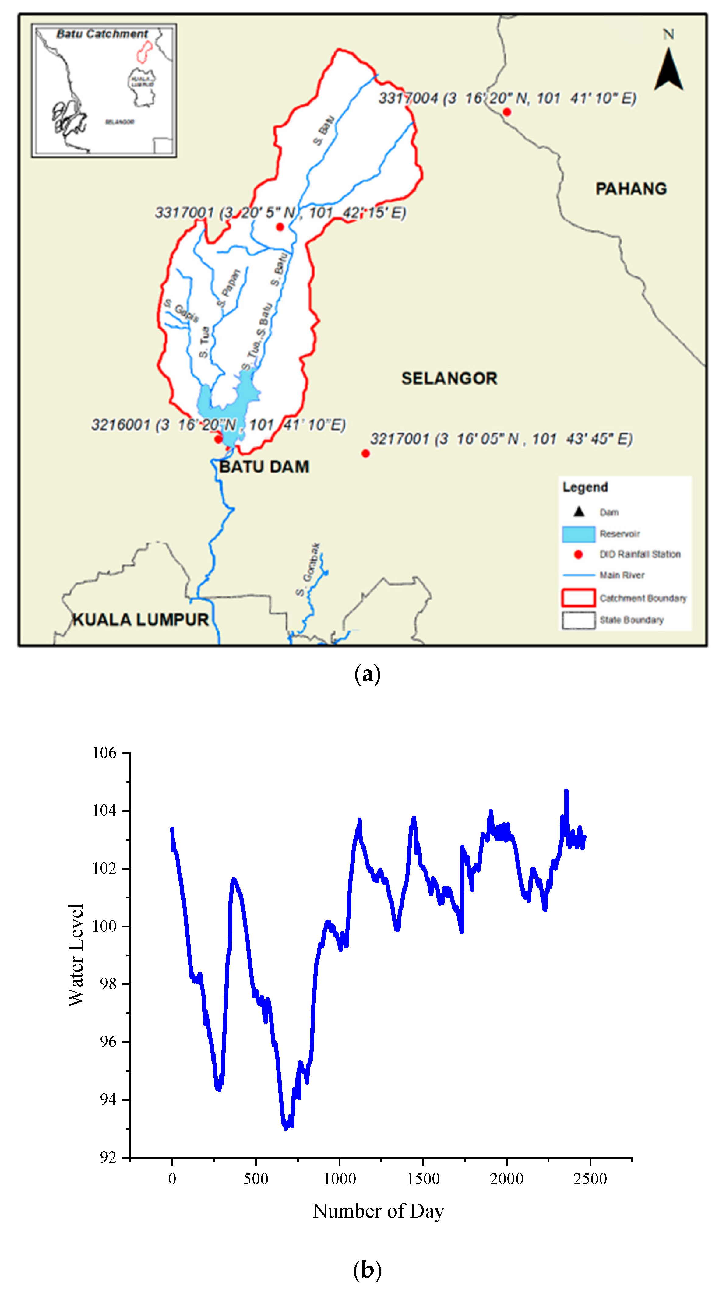
This study used the coati optimization algorithm—ELM-MKLSSVM model to predict the water reservoir level. One of the challenges is to identify the inputs for modeling hydrological processes [27]. An input variable selection method involves identifying several predictors that can explain output behavior [28]. Building inaccurate models is inevitable if meaningful predictors are overlooked [29]. In addition, large input sets lead to longer computation times for model development. There are three main types of input variable selection methods: filter-based, wrapper-based, and embedded-based [29]. A filter-based input variable selection method (FIVS) is independent of the learning algorithm and uses statistical measures to rank input variables [29,30]. Wrapper-based input variable selection (WIVS) methods and embedded input variable selection methods (EMIVS), which use a learning algorithm, filter variables based on model performance.
WIVS and EMIVS methods have high computational burdens, but they are more efficient than FIVS. A wrapper method uses a subset of features to train a model. Various wrapper methods are available, such as sequential or random [30]. The sequential wrapper method, such as the forward feature selection and backward elimination methods, incrementally adds and removes features from the selected subset. As a result, the features selected/removed in the first iteration are not removed/selected in the next iteration to improve the model’s performance [30].
In contrast to sequential wrappers, random search methods provide an enhanced technique for exploring the feature space. Optimization algorithms are the most important random search methods. A global optimization approach is used to develop wrapper input variable selection techniques where input subsets are represented as binary strings. When the search algorithm selects the i-th input, the i-th bit of the string will be set to 1; otherwise, it will be set to 0. Next, the selected predictors are fed into a machine-learning model, which is then trained and evaluated. Each individual had two parts: an input variable and a hyperparameter [28]. Hyperparameters are encoded as binary values [27]. The values of the hyperparameters and input variables were back-transformed into actual values in the final level [28]. In this study, the coot is chosen to determine the input variables. The model is created based on the following levels:
Data are split into testing and training data. The name of input variables must be converted into a binary format. Each variable is represented as a sequence of 0 s and 1 s. For example, if you have three input variables A, B, and C, you can represent each of them using two bits as follows:
A = 00 , 01 , 10 , 11 B = 00 , 01 , 10 , 11 C = 00 , 01 , 10 , 11
A binary vector contains 0 and 1 values. 0 and 1 values show unselected and selected input data. The model parameters and input vectors are defined as the population of the algorithms. The input vectors are inserted into the MKLSSVM. An objective function (MAE) is calculated to evaluate the quality of the solutions—Equations (13)–(18) update model parameters and input vectors. The process continues until the convergence criterion (maximum number of iterations) is met. Residual values are computed based on the difference between outputs and observed data. The parameters of the ELM model are defined as the initial population of the coati optimization algorithm. Residual values are inserted into the ELM model. The elm model is run to predict outputs. An objective function (Mean absolute error (MAE)) is calculated to evaluate the quality of the solutions. The operators of the coati optimization algorithm are used to update extreme learning machine parameters. Equation (22) provides the final output:
O u t f i n a l = O u t E L M + o u t M K L S S V M
where O u t f i n a l : final output, O u t E L M : output of the extreme learning machine model (estimated residual value), and o u t M K L S S V M : output of the MKLSSVM model. In this study, the ELM-MKLSSVM model is benchmarked against the LSSVM-RBF, LSSVM-LKF, LSSVM-PKF, and ELM models.

3. Case Study

The Batu Dam, located approximately 20 km north of Kuala Lumpur, is in Malaysia. Water supply, sediment management, and flood regulation are the goals of building the Batu Reservoir in Kuala Lumpur. The dam is an earth-fill embankment. Climate change affects rainfall patterns. As rainfall patterns change, reservoir inflow and water levels change. The dam’s height, length, and crest elevation are 44 m, 50 m, and 109 m, respectively. The reservoir’s storage capacity and design discharge capacities are 36.6 MCM and 251.6 m3/s (Spillway and outlet). Decision makers need to predict the reservoir’s water level for flood control. A humid climate prevails in the basin. Figure 1a,b show the location of the case study and the data points.
This study uses lagged rainfall and water level to predict a one-day-ahead water level. Lag times of (t−1) (previous day), (t−10) (last ten days) are used for predicting outputs. Table 1 shows statistical details of inputs and outputs.
Equations (23)–(25) are used to evaluate the performance of the models.
1
Root mean square error (RMSE)
R M S E = 1 n i = 1 n W L e s W L o b 2
2
Mean absolute error (MAE)
M A E = 1 n i = 1 n W L o b W L e s
3
Nash–Sutcliff efficiency (NSE)
N S E = 1 i = 1 n W L o b W L e s 2 i = 1 n W L o b W L ¯ o b
4
Willmott index
W I = 1 i = 1 n W L e s W L o b 2 i = 1 n W L e s W L ¯ o b + W L e s W L ¯ o b 2
where, W L e s : Estimated Water level, W L o b : Observed Water Level, W L ¯ o b : Average observed Water level, n: number of data. Ideal models have high WI and NSE values.

4. Results and Discussion

4.1. Determination of Optimal Input Scenario

By reducing the number of input variables, feature selection methods can help prevent overfitting. Too many input variables can make the model overly complex and inconsistent. Overfitting occurs when a model fits training data well but performs poorly on new data. A feature selection method reduces the overfitting risk by selecting only relevant input variables. Furthermore, feature selection methods can identify redundant or irrelevant variables. Choosing the best input scenario is complex. This study uses COA to determine optimal input scenarios. The number of input variables was 20 (Rainfall (t−1)… Rainfall (t−10); Water level (t−10), … Water level (t−10)). The number of input combinations is 220-1. Manually determining the optimal input scenario is time-consuming and complex. In this study, the COA automatically determine the best input combination. The name of the input variables was defined as binary variables. The names of the input variables were considered decision variables. Locations of coatis show input combinations. The operators of the COA were used to update the input combinations at each iteration. Table 2 shows the first-best to third-best input combinations.

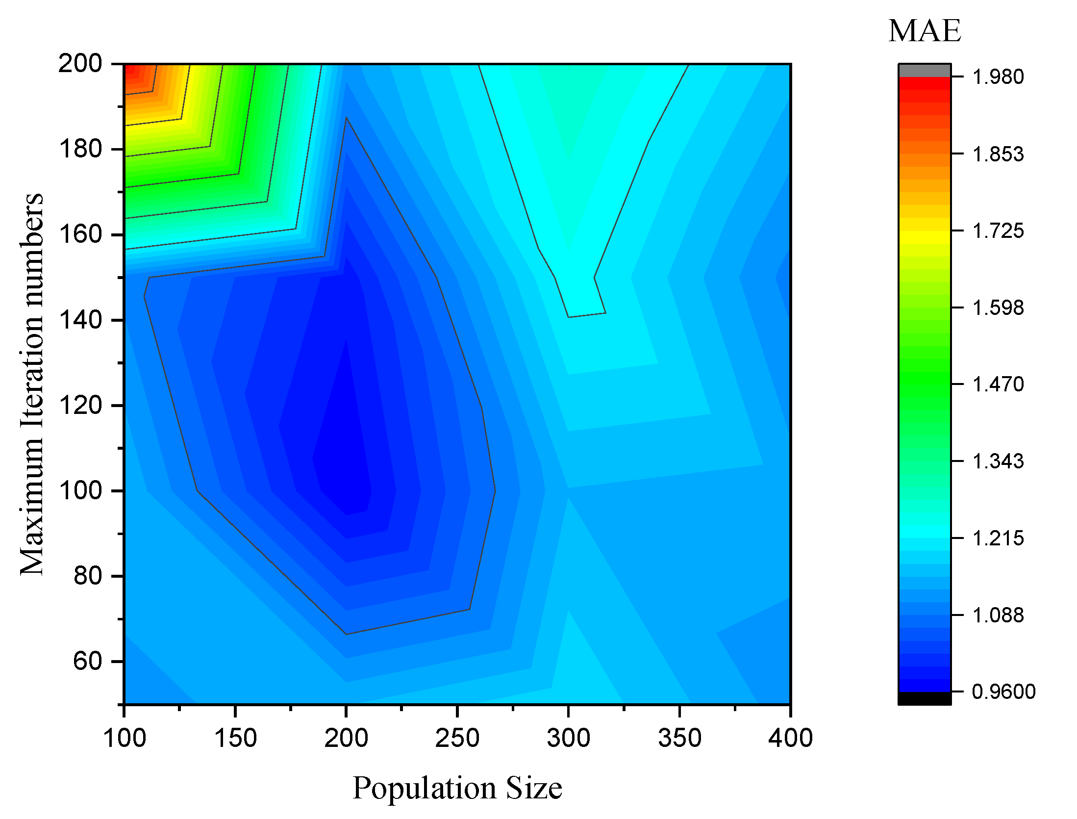
4.2. Determination of Random Parameters

The performance of an optimization algorithm depends on random parameters. Population size and maximum iteration number are the most important parameters of optimization algorithms (Figure 2). The optimal values of random parameters yield the lowest objective function values (MAE). Figure 2 shows the objective function value for different parameter values. As can be seen from the figure, population size = 200 and maximum iteration number = 100 provided the lowest objective function value.
In this study, the number of hidden nodes (N = 1,…, 256) and the type of activation function (sigmoid, sine, purelin, and radial basis) are the parameters of the ELM model. The number of hidden neurons variable varies from 1 to 256. Thus, there were 8 bits for the encoding. Since the ELM model had four activations, we used two bits for activation functions. Therefore, we needed 10 bits for the ELM parameters. At each iteration, the operators of the coot optimization algorithm updated the values of the model parameters. Based on multiple runs, the model with the best fitness was selected. Based on this selected model, the final prediction values were calculated. A matlabe software was used to prepare computer codes. Also, the ram of the system was 8 GB.

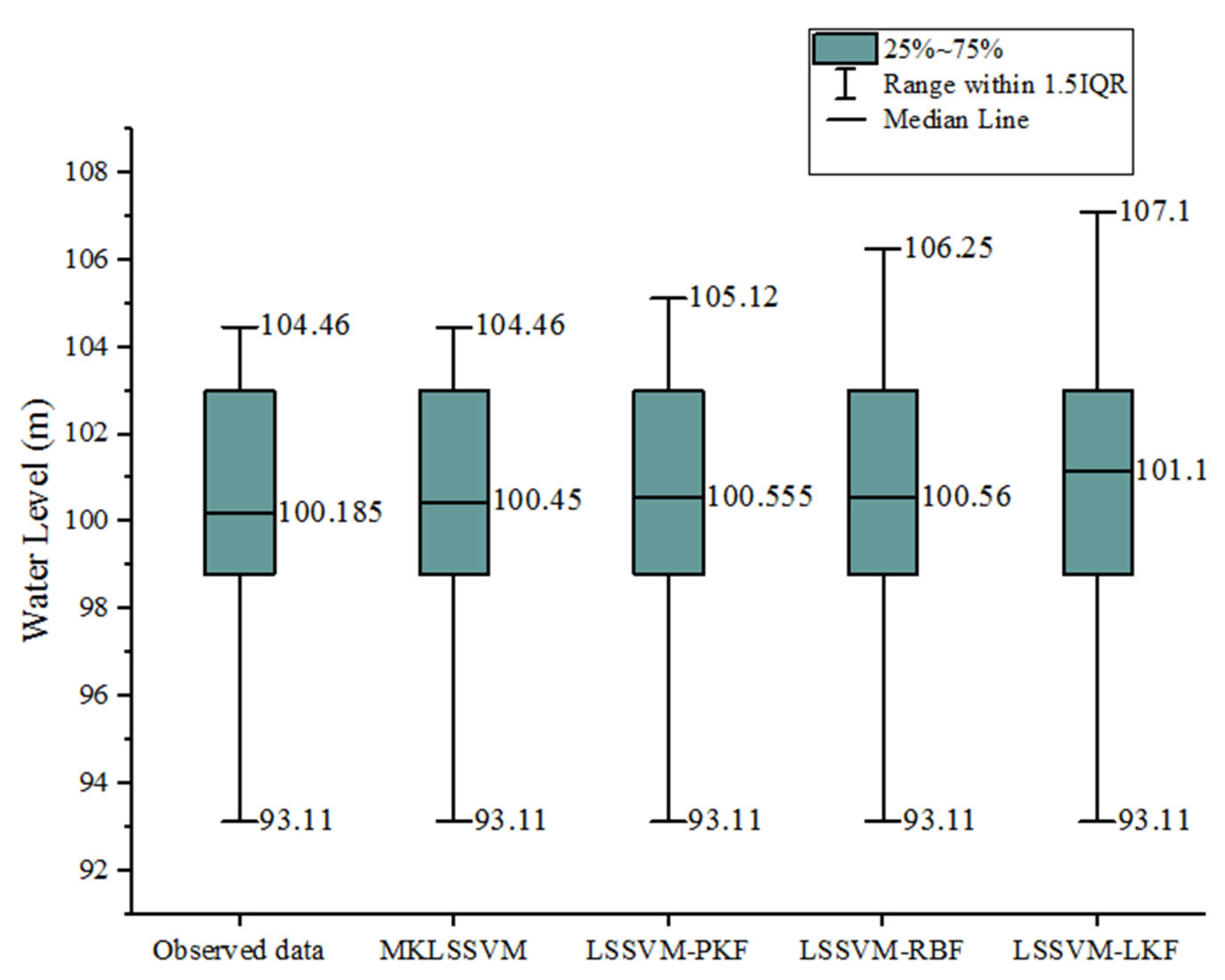
4.3. Evaluation of the Accuracy of LSSVM Models

The accuracy of the MKLSSVM, LSSVM-PKF, LSSVM-RBF, and LSSVM-LKF models is evaluated in this section (Table 3).
Table 3 evaluates the accuracy of different LSSVM models. The highest and Lowest MAEs were obtained by the LSSVM-LKF and MKLSSVM models. The training and testing MAEs of the MKLSSVM model were 0.96 and 0.99, respectively. The LSSVM-PKF model was the second-best. The training and testing MAEs of the LSSVM-PKF were 1.02 and 1.12, respectively.
The NSE of the LSSVM-LKF model was lower than that of the other models. The training and testing NSE of the MKLSSVM model was 0.79 and 0.78, respectively. On the other hand, the LSSVM-RBF outperformed the LSSVM-LKF model. The training and testing NSE of the LSSVM-RBF model was 0.76 and 0.74.
The training RMSE of the MKLSSVM model was 15 and 16% was lower than that of the LSSVM-PKF and LSSVM-RBF models. On the other hand, the RMSE of the LSSVM-LKF was higher than that of the other models. The training and testing RMSE of the LSSVM-LKF were 2.12 and 2.24, respectively.
The WI of the MKLSSVM model was higher than that of the models. The training and testing WIs of the MKLSSVM model were 0.80 and 0.79, respectively. The WI of the LSSVM-KF was higher than that of the other models.
Figure 3 shows boxplots of the LSSVM models. The observed data had the highest match with the MKLSSVM model. The median and maximum values of the observed data were 100.185 and 104.46 m, respectively. The median and maximum values of the MKLSSVM model were 100.45 and 104.46. On the other hand, the LSSVM-LKF had the lowest match with the observed data. The median and maximum values of the LSSVM-LKF model were 101.1 and 107.1 m, respectively.
Among the other models, LSSVM-LKF had the lowest accuracy. The LSSVM-LKF model is poor for analyzing nonlinear data because it uses a linear kernel function. The LSSVM-PKF (RBF) use nonlinear kernel functions, so they perform better than the LSSVM-LKF model. Since the MKLSSVM model takes advantage of multiple kernel functions, it can predict data accurately. The performance of LSSVM models improves as the exponent increases. The least LSSVM-PKF model performed better than the least square support vector machine—RBF model.

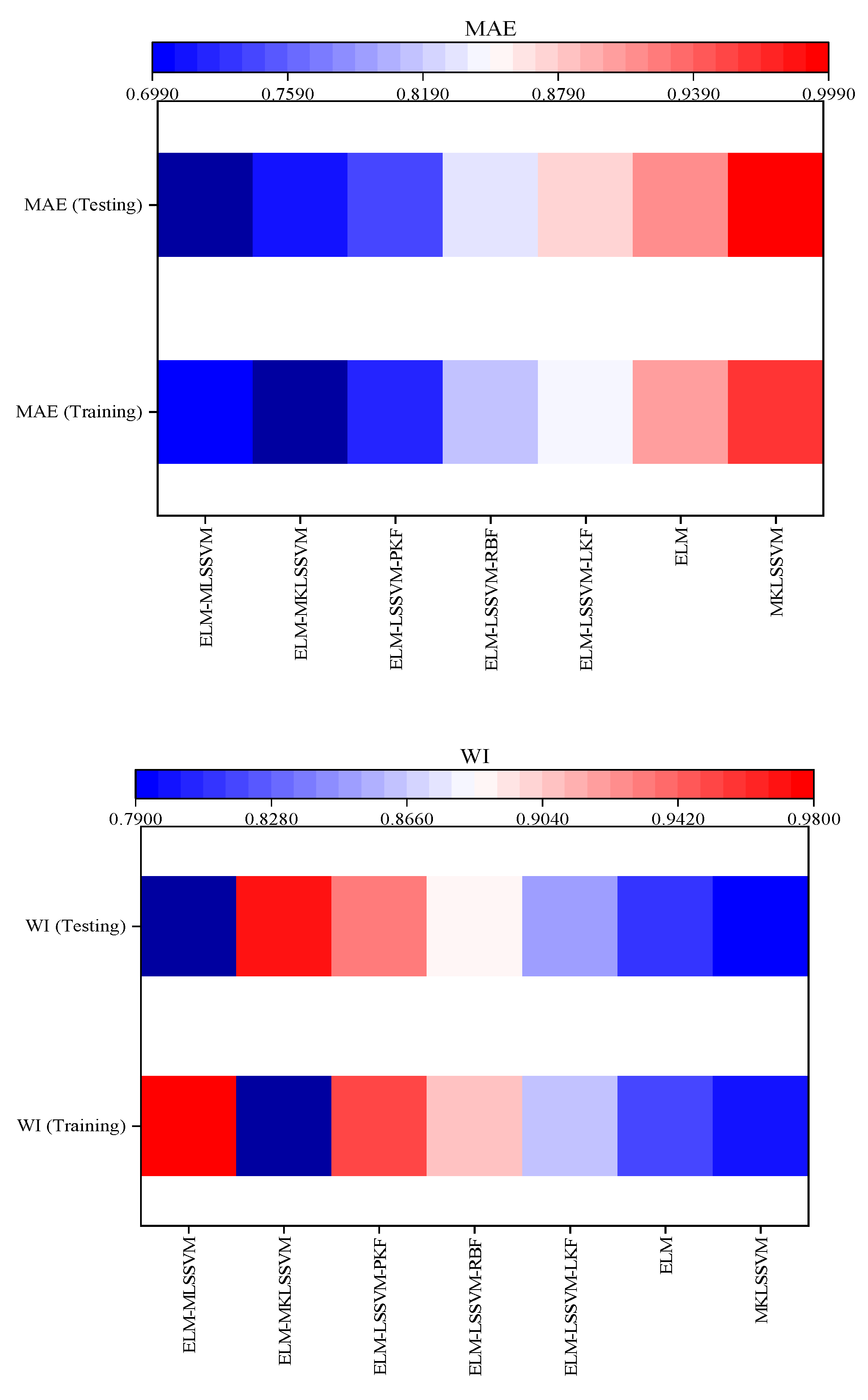
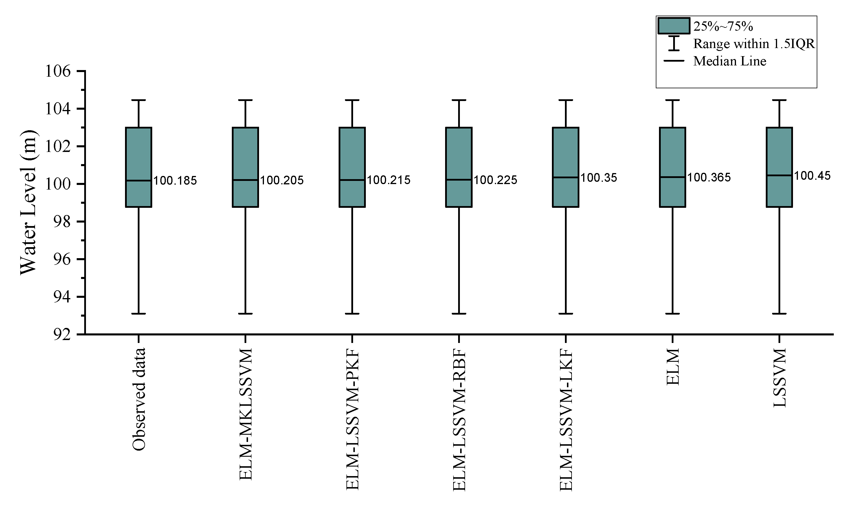
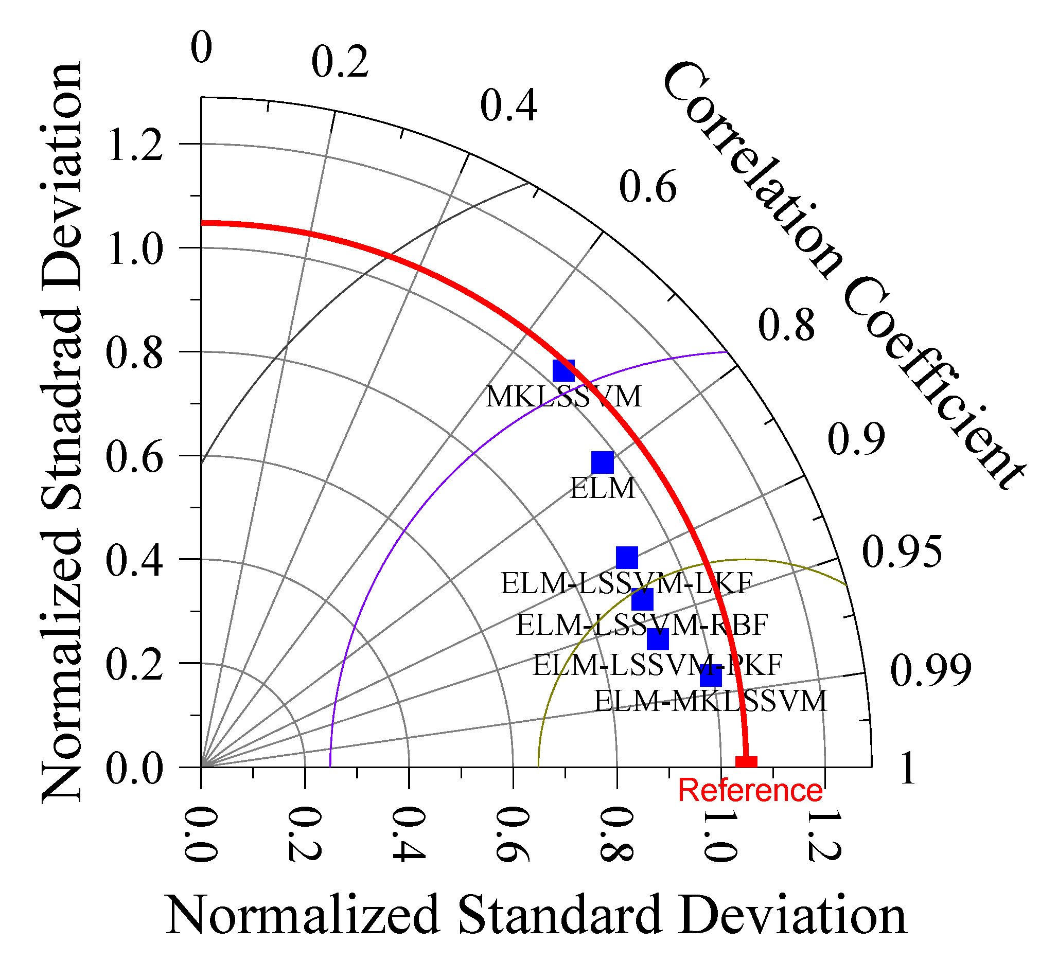
4.4. Evaluation of the Accuracy of Hybrid Models

In this section, the ELM-MKLSSVM model is benchmarked against other models. Figure 4 shows heat maps of error values. The MKLSSVM had the highest RMSE. The training and testing RMSEs of the MKLSSVM model were 52% and 54% higher than those of the ELM-MKLSSVM model. The training and testing RMSEs of the ELM-MKLSSVM model were 0.858 and 0.912 m, respectively. The ELM-MKLSSVM decreased RMSE values of the ELM model by 15% and 17%, respectively.
The highest NSE was obtained by the ELM-MKLSSVM model. The training and testing NSEs of the ELM-MKLSSVM model were 0.98 and 0.97, respectively. Therefore, the NSE of the ELM was higher than that of the MKLSSVM model. The training and testing of NSEs of the ELM-RBF model were higher than those of the ELM-LLSVM-PKF model. The training and testing NSEs of the ELM-RBF model were 0.92 and 0.90, respectively.
The WI of the ELM-MKLSSVM model was 0.98 and 0.97 at the training and testing level. The WI of the ELM-MKLSSVM model was higher than that of the other models. The WI values indicated that the ELM-LSSVM-PKF was the second-best model. The training and testing WIs of the same model were 0.95 and 0.93. The NSE of the same model was lower than that of the ELM-MKLSSVM model. The MAE of the ELM was higher than that of the ELM-MKLSSVM models. The training and testing MAEs of the ELM model were 0.901 and 0.912, respectively. The training and testing MAEs of the MKLSSV model were 0.70 and 0.71, respectively. The testing MAE of the ELM-MKLSSVM model was 28% lower than that of the MKLSSVM model.
Since the ELM-MKLSSVM model combines the advantages of the extreme learning machine and MKLSSVM models, it outperforms other models. While the LSSVM model may not capture nonlinear components of time series data, the ELM-MKLSSVM model can capture both nonlinear and linear components. The results showed that hybrid models performed better than MKLSSVM and ELM models. Figure 5 shows boxplots of hybrid and standalone LSSVM and ELM models. The median of the observed data and the ELM-MKLSSVM model had the highest match. The medians of the observed data and the ELM-MKLSSVM model were 100.185 m and 100.205 m, respectively. The ELM and MKLSSVM model median was 100.385 and 100.450 m, respectively. Thus, these models had weaker performance than the ELM-MKLSSVM model. A Taylor diagram is used to evaluate the accuracy of a model. For evaluating the accuracy of models, the Taylor diagram uses standard deviation, correlation coefficient, and the centralized root mean square error (CRMSE). The ideal model has the shortest distance from the reference point (observed data). Figure 6 shows a Taylor diagram for assessing the accuracy of hybrid and standalone LSSVM models. The CRMSE of the hybrid models was lower than that of the standalone models (ELM and MKLSSVM models). The CRMSE of the ELM-MKLSSVM model and ELM-LSSVM-PKF was 0.17 and 0.27, respectively. The correlation coefficient of the same models was 0.98 and 0.96. The correlation coefficient of the MKLSSVM model was 0.67.
Predicting reservoir water levels is a key issue in managing agricultural, industrial, and domestic water resources. Therefore, a reliable predictive model is required to ensure an adequate water supply.
This study used the ELM-MKLSSVM model to estimate reservoir water levels. Our study results are important for water management. First, water managers can allocate reservoir water to different uses based on accurately predicting reservoir water levels. For example, water may be allocated to agricultural or urban areas for drinking, cleaning, or other purposes. Secondly, the study results help predict and prevent natural disasters such as floods. Dam overflow can occur when the reservoir water level increases uncontrollably, which can cause havoc in surrounding areas. Water level predictions and early warnings can help people and institutions move to safer places before natural hazards occur. Thirdly, study results are essential for planning the construction and operation of hydropower plants. The reservoir water level determines the amount of electricity that can be generated. Therefore, accurately predicting the reservoir water level can help prevent power outages and maintain a stable power supply. Fourth, water can damage land, crops, and infrastructure during a flood or overflow. The accurate prediction of water levels helps communities prepare for flood events that can cause destruction. A drought puts pressure on reservoirs because demand increases and water supply decreases. As precipitation decreases and evaporation rates increase, the reservoir water level falls, causing water scarcity, ecosystem damage, and socioeconomic impacts. Water scarcity can adversely affect agriculture, threaten water supply and hydroelectric power generation, and cause financial losses. To minimize the effect of water scarcity on water user economies and to maintain stability for water users, water resource managers must make accurate predictions of reservoir water levels.
In this study, we used the ELM model to improve the performance of the MKLSSVM model. The extreme learning machine is a supervised learning algorithm for neural networks for regression and classification tasks. Due to its simplicity, high-speed processing, and accuracy, the ELM model is a powerful machine-learning technique. ELM models are advantageous for predicting the water level of reservoirs because they can process large amounts of data. An ELM model can employ many hidden neurons to learn the complexity of the reservoir systems, which leads to better accuracy in predicting water levels. In addition, an ELM model has a fast-learning ability with a shorter training time.
When the extreme learning machine—MKLSSVM model receives the climate information, it can predict the water level for the feature periods. Climate models and scenarios can be coupled with the ELM-MKLSSVM model to predict water levels for future periods. The ELM-MKLSSVM model can be used for predicting other variables (rainfall, groundwater level, and temperature) as it can capture nonlinear and linear components. Furthermore, our study contributed to the development of robust feature selection algorithms. The COA was a robust feature selection tool.
In order to increase the accuracy of predictive models, the coot optimization algorithm selected the most relevant input variables. Models that contain irrelevant or redundant variables often produce incorrect predictions. The coot optimization could reduce the computational complexity of predictive models by eliminating unnecessary input variables. As a result, model training and prediction can be faster and more efficient. Choosing input variables relevant to the target variable improves the interpretability of predictive models. By understanding the relationship between input and output variables, users can make informed decisions. In addition to improving the accuracy of predictive models, optimization algorithms improve their generalization.
There are several reasons why multi-kernel least square support vector machines (MKLSSVMs) perform better than LSSVMs. First, the MKLSSVM model can combine multiple kernels, which makes it flexible for fitting different types of data distributions. In contrast, the LSSVM model uses a single kernel function, which can not capture the complexity of data. When the MKLSSVM model uses multiple kernels, regularization occurs, which will reduce model overfitting. When the kernel function is not selected properly, LSSVM may be more prone to overfitting. The MKLSSVM model can improve the generalization ability to perform well on unseen data samples. In other words, using multiple kernels leads to a more robust and diverse model. When the input data are highly nonlinear and complex, LSSVM may have poor generalization ability. MKLSSVM can often achieve higher accuracy because it can capture more complex data patterns than LSSVM. It is particularly true for datasets that contain many features or high dimensionality. Finally, the LSSVM model can handle large datasets. Many applications have datasets with a large number of data points. Due to their reliance on a single kernel function, traditional LSSVM models can be computationally expensive or impossible to train on such large datasets. The MKLSSVM model can distribute the computation across multiple kernel functions for large datasets, making it more efficient and scalable. Previous studies reported that the combination of kernel functions could improve the accuracy of results. Ghiasi et al. [32] developed the LSSVM models based on the combination of kernel functions. They reported that the new model could successfully predict structural damage detection. Zhou et al. [33] developed a combination of kernel functions for the LSSVM model. The combination of kernel functions could improve the accuracy of the original LSSVM model.
The limitation of our models is that time interval predictions cannot be quantified. To quantify uncertainty values, it is necessary to make time interval predictions. We can develop our models for quantifying uncertainty values in the next studies. Modelers need skill and experience to prepare such models. Data collection can be challenging because some data may not be available. Combining multiple models requires careful integration and coordination, which can be challenging for developers to implement.
These models provide useful results for the optimal management of the Batu Dam. Water level predictions help reservoir managers understand the status of reservoir storage. Thus, water can be released based on reservoir water levels and downstream demands. During periods of drought, managers can use these models for watershed management. As reservoir water levels can be accurately predicted, managers can optimally open the Batu dam and release water during periods of drought. The Batu Dam provides water for domestic and industrial use, irrigation, and power generation. Thus, this dam is important for the water supply. Our models predict reservoir water levels so that managers can plan for the optimal operation of Batu. Dam. As a result, our models contribute to improving dam management. We propose these models as early warning systems to prevent floods and droughts in the catchment area. Furthermore, we propose water resource management under climate change conditions.

5. Conclusions

Predicting reservoir water levels is vital for effective water management. Predicting reservoir water levels also facilitates flood management. Heavy rainfall can cause significant damage to the environment, infrastructure, and human life when reservoirs overflow. To prevent floods and disasters, water resource managers can use reservoir water level predictions. For environmental management, it is important to predict reservoir water levels. A water resource manager must balance the needs of different sectors and environmental protection. During the dry season, water resource managers may need to limit water allocations for some sectors to meet downstream needs. Predicting reservoir water levels allows managers to plan for environmental flows and adjust water allocations.
Predicting water reservoir levels can mitigate the consequences of floods and droughts. This study aims to develop a new hybrid model for predicting the water level of reservoirs. Our study coupled the MKLSSVM model with the ELM model. The MKLSSVM model is a new version of the LSSVM model. The multi-kernel least square support vector machine model takes advantage of multiple kernel functions. For selecting the optimal input scenarios, we used a new binary optimization algorithm. The results indicated that the extreme learning machine—multi-kernel least square support vector machine model outperformed the other models.
The highest NSE was obtained by the ELM-MKLSSVM model. The training and testing NSEs of the ELM-MKLSSVM model were 0.98 and 0.97, respectively. The training and testing NSE of the MKLSSVM model was 0.79 and 0.78, respectively. The LSSVM-RBF outperformed the LSSVM-LKF model. The training and testing NSEs of the ELM-RBF model were 0.92 and 0.90, respectively.
Our study showed that the extreme learning machine—MKLSSVM was a reliable tool for analyzing linear and nonlinear data. The new model can provide valuable information for water resource planning and management. Researchers can use the new model to predict spatial and temporal patterns. Choosing the essential input variables is complex, but our optimization algorithm selects them successfully. This article used a hybrid model to predict nonlinear and linear components of time series. This idea can be used to develop the performance of other models, such as support vector machines, regression models, and linear models.
The ELM-MKLSSVM is a robust model for simulating complex problems but cannot predict interval times. We can combine the ELM-MKLSSVM model with Bayesian approaches to predict interval times in the next study. Quantifying uncertainty values relies on interval-time predictions.

Author Contributions

Conceptualization, S.S.S. and M.E.; methodology, M.E. and Z.S.K.; software, L.M.S.; validation, S.S.S., Z.S.K. and M.E.; formal analysis, M.E. and Z.S.K.; investigation, Z.S.K.; resources, Z.S.K.; data curation, S.S.S. and L.M.S.; writing—original draft preparation, M.E.; writing—review and editing, M.E. All authors have read and agreed to the published version of the manuscript.

Funding

The research work is funded by the project, the Transdisciplinary Research Grant Scheme (TRGS) of Grant No. TRGS/1/2020/UNITEN/01/1/1 of Ministry of Higher Education (MoHE), Malaysia.

Institutional Review Board Statement

Not applicable.

Informed Consent Statement

Not applicable.

Data Availability Statement

The datasets generated during the current study are available for other researchers upon reasonable request.

Conflicts of Interest

The authors declare no conflict of interest.

References

  1. Kusudo, T.; Yamamoto, A.; Kimura, M.; Matsuno, Y. Development and Assessment of Water-Level Prediction Models for Small Reservoirs Using a Deep Learning Algorithm. Water 2022, 14, 55. [Google Scholar] [CrossRef]
  2. Ren, T.; Liu, X.; Niu, J.; Lei, X.; Zhang, Z. Real-time water level prediction of cascaded channels based on multilayer perception and recurrent neural network. J. Hydrol. 2020, 585, 124783. [Google Scholar] [CrossRef]
  3. Azad, A.S.; Sokkalingam, R.; Daud, H.; Adhikary, S.K.; Khurshid, H.; Mazlan, S.N.A.; Rabbani, M.B.A. Water Level Prediction through Hybrid SARIMA and ANN Models Based on Time Series Analysis: Red Hills Reservoir Case Study. Sustainability 2022, 14, 1843. [Google Scholar] [CrossRef]
  4. Park, K.; Jung, Y.; Seong, Y.; Lee, S. Development of Deep Learning Models to Improve the Accuracy of Water Levels Time Series Prediction through Multivariate Hydrological Data. Water 2022, 14, 469. [Google Scholar] [CrossRef]
  5. Guo, T.; He, W.; Jiang, Z.; Chu, X.; Malekian, R.; Li, Z. An Improved LSSVM Model for Intelligent Prediction of the Daily Water Level. Energies 2019, 12, 112. [Google Scholar] [CrossRef]
  6. Tang, Y.; Zang, C.; Wei, Y.; Jiang, M. Data-Driven Modeling of Groundwater Level with Least-Square Support Vector Machine and Spatial–Temporal Analysis. Geotech. Geol. Eng. 2019, 37, 1661–1670. [Google Scholar] [CrossRef]
  7. Moravej, M.; Amani, P.; Hosseini-Moghari, S.-M. Groundwater level simulation and forecasting using interior search algorithm-least square support vector regression (ISA-LSSVR). Groundw. Sustain. Dev. 2020, 11, 100447. [Google Scholar] [CrossRef]
  8. Noorain, I.S.; Ismail, S.; Sadon, A.N.; Yasin, S.M. Application of box-jenkins, artificial neural network and support vector machine model for water level prediction. In Recent Advances in Soft Computing and Data Mining, Proceedings of the Fifth International Conference on Soft Computing and Data Mining (SCDM 2022), Virtual Event, 30–31 May 2022; Springer International Publishing: Cham, Switzerland, 2022; pp. 121–130. [Google Scholar]
  9. Bemani, A.; Xiong, Q.; Baghban, A.; Habibzadeh, S.; Mohammadi, A.H.; Doranehgard, M.H. Modeling of cetane number of biodiesel from fatty acid methyl ester (FAME) information using GA-, PSO-, and HGAPSO-LSSVM models. Renew. Energy 2020, 150, 924–934. [Google Scholar] [CrossRef]
  10. Pham, Q.B.; Yang, T.C.; Kuo, C.M.; Tseng, H.W.; Yu, P.S. Combing Random Forest and Least Square Support Vector Regression for Improving Extreme Rainfall Downscaling. Water 2019, 11, 451. [Google Scholar] [CrossRef]
  11. Miranian, A.; Abdollahzade, M. Developing a Local Least-Squares Support Vector Machines-Based Neuro-Fuzzy Model for Nonlinear and Chaotic Time Series Prediction. IEEE Trans. Neural Netw. Learn. Syst. 2013, 24, 207–218. [Google Scholar] [CrossRef]
  12. Gong, W.; Tian, S.; Wang, L.; Li, Z.; Tang, H.; Li, T.; Zhang, L. Interval prediction of landslide displacement with dual-output least squares support vector machine and particle swarm optimization algorithms. Acta Geotech. 2022, 17, 4013–4031. [Google Scholar] [CrossRef]
  13. Yuan, X.; Chen, C.; Yuan, Y.; Huang, Y.; Tan, Q. Short-Term Wind Power Prediction Based on LSSVM-GSA Model. Energy Convers. Manag. 2015, 101, 393–401. [Google Scholar] [CrossRef]
  14. Chia, S.L.; Chia, M.Y.; Koo, C.H.; Huang, Y.F. Integration of advanced optimization algorithms into least-square support vector machine (LSSVM) for water quality index prediction. Water Supply 2022, 22, 1951–1963. [Google Scholar] [CrossRef]
  15. Shiri, J.; Shamshirband, S.; Kisi, O.; Karimi, S.; Bateni, S.M.; Nezhad, S.H.H.; Hashemi, A. Prediction of Water-Level in the Urmia Lake Using the Extreme Learning Machine Approach. Water Resour. Manag. 2016, 30, 5217–5229. [Google Scholar] [CrossRef]
  16. Deo, R.C.; Şahin, M. An extreme learning machine model for the simulation of monthly mean streamflow water level in eastern Queensland. Environ. Monit. Assess. 2016, 188, 90. [Google Scholar] [CrossRef] [PubMed]
  17. Fabio, D.N.; Abba, S.I.; Pham, B.Q.; Islam, A.R.M.T.; Talukdar, S.; Francesco, G. Groundwater level forecasting in Northern Bangladesh using nonlinear autoregressive exogenous (NARX) and extreme learning machine (ELM) neural networks. Arab. J. Geosci. 2022, 15, 647. [Google Scholar] [CrossRef]
  18. Ardabili, S.F.; Najafi, B.; Alizamir, M.; Mosavi, A.; Shamshirband, S.; Rabczuk, T. Using SVM-RSM and ELM-RSM Approaches for Optimizing the Production Process of Methyl and Ethyl Esters. Energies 2018, 11, 2889. [Google Scholar] [CrossRef]
  19. Bonakdari, H.; Ebtehaj, I.; Samui, P.; Gharabaghi, B. Lake Water-Level fluctuations forecasting using Minimax Probability Machine Regression, Relevance Vector Machine, Gaussian Process Regression, and Extreme Learning Machine. Water Resour. Manag. 2019, 33, 3965–3984. [Google Scholar] [CrossRef]
  20. Seidu, J.; Ewusi, A.; Kuma, J.S.Y.; Ziggah, Y.Y.; Voigt, H.-J. A hybrid groundwater level prediction model using signal decomposition and optimised extreme learning machine. Model. Earth Syst. Environ. 2022, 8, 3607–3624. [Google Scholar] [CrossRef]
  21. Zhang, G.; Liu, H.; Li, P.; Li, M.; He, Q.; Chao, H.; Zhang, J.; Hou, J. Load Prediction Based on Hybrid Model of VMD-mRMR-BPNN-LSSVM. Complexity 2020, 2020, 6940786. [Google Scholar] [CrossRef]
  22. Ahmadi, M.H.; Sadatsakkak, S.A.; Feidt, M. Connectionist intelligent model estimates output power and torque of stirling engine. Renew. Sustain. Energy Rev. 2015, 50, 871–883. [Google Scholar] [CrossRef]
  23. Zhang, Y.; Le, J.; Liao, X.; Zheng, F.; Li, Y. A novel combination forecasting model for wind power integrating least square support vector machine, deep belief network, singular spectrum analysis and locality-sensitive hashing. Energy 2019, 168, 558–572. [Google Scholar] [CrossRef]
  24. Yaseen, Z.M.; Sulaiman, S.O.; Deo, R.C.; Chau, K.-W. An enhanced extreme learning machine model for river flow forecasting: State-of-the-art, practical applications in water resource engineering area and future research direction. J. Hydrol. 2019, 569, 387–408. [Google Scholar] [CrossRef]
  25. Akyol, S.; Alatas, B. Plant intelligence based metaheuristic optimization algorithms. Artif. Intell. Rev. 2017, 47, 417–462. [Google Scholar] [CrossRef]
  26. Dehghani, M.; Montazeri, Z.; Trojovská, E.; Trojovský, P. Coati Optimization Algorithm: A new bio-inspired metaheuristic algorithm for solving optimization problems. Knowl.-Based Syst. 2023, 259, 110011. [Google Scholar] [CrossRef]
  27. Taormina, R.; Chau, K.-W. Data-driven input variable selection for rainfall–runoff modeling using binary-coded particle swarm optimization and Extreme Learning Machines. J. Hydrol. 2015, 529, 1617–1632. [Google Scholar] [CrossRef]
  28. Ren, K.; Wang, X.; Shi, X.; Qu, J.; Fang, W. Examination and comparison of binary metaheuristic wrapper-based input variable selection for local and global climate information-driven one-step monthly streamflow forecasting. J. Hydrol. 2021, 597, 126152. [Google Scholar] [CrossRef]
  29. Qu, J.; Ren, K.; Shi, X. Binary Grey Wolf Optimization-Regularized Extreme Learning Machine Wrapper Coupled with the Boruta Algorithm for Monthly Streamflow Forecasting. Water Resour. Manag. 2021, 35, 1029–1045. [Google Scholar] [CrossRef]
  30. Agrawal, R.; Kaur, B.; Sharma, S. Quantum based Whale Optimization Algorithm for wrapper feature selection. Appl. Soft Comput. 2020, 89, 106092. [Google Scholar] [CrossRef]
  31. Omar, S.M.A.; Ariffin, W.N.H.W.; Sidek, L.M.; Basri, H.; Khambali, M.H.M.; Ahmed, A.N. Hydrological Analysis of Batu Dam, Malaysia in the Urban Area: Flood and Failure Analysis Preparing for Climate Change. Int. J. Environ. Res. Public Health 2022, 19, 16530. [Google Scholar] [CrossRef]
  32. Ghiasi, R.; Torkzadeh, P.; Noori, M. A machine-learning approach for structural damage detection using least square support vector machine based on a new combinational kernel function. Struct. Health Monit. 2016, 15, 302–316. [Google Scholar] [CrossRef]
  33. Zhu, B.; Ye, S.; Wang, P.; Chevallier, J.; Wei, Y. Forecasting carbon price using a multi-objective least squares support vector machine with mixture kernels. J. Forecast. 2022, 41, 100–117. [Google Scholar] [CrossRef]
Figure 1. (a) Location of the case study [31], (b) Time series data.
Water 15 01593 g001
Figure 2. Values of the objective function for different values of parameters.
Water 15 01593 g002
Figure 3. Boxplots of the MKLSSVM and different least square support vector machine models.
Water 15 01593 g003
Figure 4. Heat maps of error values.
Water 15 01593 g004aWater 15 01593 g004b
Figure 5. Boxplots of hybrid LSSVM models.
Water 15 01593 g005
Figure 6. Comparison of the accuracy of models based on the Taylor diagram.
Water 15 01593 g006
Table 1. Statistical details of data.
ParameterMaximum Average Minimum
Water Level (m)104.46 99.23 93.11
Rainfall (mm)50.534.560.50
Table 2. The best input combinations.
Input CombinationComponents
First best input combination rainfall (t−1), rainfall (t−2), water level (t−1), water level (t−2), water level (t−3)
Second best input combination rainfall (t−1), rainfall (t−2), water level (t−1), water level (t−2), water level (t−3), rainfall (t−4)
Third-best input combination rainfall (t−1), rainfall (t−2), water level (t−1), water level (t−2), water level (t−3), rainfall (t−3), water level (t−5)
Table 3. Investigation of the accuracy of the LSSVM models.
Model MAE (Training)MAE
(Testing)
RMSE
(Training)
RMSE
(Testing)
NSE
(Training)
NSE
(Testing)
WI
(Training)
WI
(Testing)
MKLSSVM0.960.991.671.780.790.780.800.79
LSSVM-PKF1.021.121.971.980.770.770.780.76
LSSVM-RBF1.141.231.992.010.760.740.750.74
LSSVM-LKF1.181.282.122.240.730.720.730.71
Disclaimer/Publisher’s Note: The statements, opinions and data contained in all publications are solely those of the individual author(s) and contributor(s) and not of MDPI and/or the editor(s). MDPI and/or the editor(s) disclaim responsibility for any injury to people or property resulting from any ideas, methods, instructions or products referred to in the content.

