
Assessing the Effect of Conduit Pattern and Type of Recharge on the Karst Spring Hydrograph: A Synthetic Modeling Approach

1
Department of Earth Sciences, Faculty of Sciences, Shiraz University, Shiraz P.O. Box 71348-14336, Iran
2
Department of Science and Technology, University of Sannio, Via dei Mulini 59/A, 82100 Benevento, Italy
*
Author to whom correspondence should be addressed.
Water 2023, 15(8), 1594; https://doi.org/10.3390/w15081594
Submission received: 5 March 2023
/
Revised: 7 April 2023
/
Accepted: 13 April 2023
/
Published: 19 April 2023
(This article belongs to the Section Hydrogeology)
Abstract
:It is widely accepted that spring hydrographs are an effective tool for evaluating the internal structure of karst aquifers because they depict the response of the whole aquifer to recharge events. The spring hydrograph is affected by various factors such as flow regime, geometry, type of recharge, and hydraulic properties of conduit. However, the effect of conduit network geometry received less attention and required more comprehensive research studies. The present study attempted to highlight the impact of the two most frequent patterns of karst conduits (i.e., branchwork and network maze) on the characteristic of the spring hydrograph. Therefore, two conduit patterns, branchwork and network maze, were randomly generated with MATLAB codes. Then, MODFLOW-CFP was used to quantify the effect of conduit pattern, conduit density, and diffuse or concentrated recharge on the spring hydrograph. Results reveal that peak discharge, fast-flow recession coefficient, and the return time to baseflow are mainly affected by conduit network pattern, conduit network density, and recharge, respectively. In contrast, the time to reach peak flow only reacts to recharge conditions. Large variations in conduit density produce tangible changes in the baseflow recession coefficient.
Highlights:
- The network maze conduit pattern is generated based on a newly developed code.
- A synthetic modeling approach is applied to characterize the shape of the spring hydrograph.
- The interaction of conduit patterns and recharge types mainly affects the spring hydrograph.
- Peak discharge and time are controlled by conduit patterns and recharge events, respectively.
- The recession coefficient is mainly affected by the density of conduits.
1. Introduction
Karst water resources play a crucial role on a worldwide scale since 20–25% of the world’s population relies on water from these areas [1]. Karst aquifers are characterized by sinkholes, conduits, springs, and drainage systems due to dissolution, internal drainage, and collapse [2]. Karst systems are a complex and heterogeneous medium due to the simultaneous influence of various geological, hydrogeological, and chemical factors in their development and evolution [3,4]. Karst aquifers are complex due to their inherent heterogeneity, which has made it hard to determine their function [5]. However, karst aquifers have been considered a medium with double porosity (conduit and matrix) or triple porosity (conduit, fracture, and matrix). Their main characteristic is triple porosity, leading to different flow and storage in the matrix, channels, and fractures [6].
Moreover, the heterogeneity from developing the karst conduit network is not comparable to heterogeneous porous media and fractured limestone aquifers. As a result of karst development processes, several inception karst horizons, such as major discontinuities, joints, fractures, and bedding planes, create a hydraulic connection from the karst surface features to discharging points, such as major springs. The heterogeneity of karst systems gradually organizes and develops, becoming an integrated drainage system similar to hierarchical river systems [7].
Due to the heterogeneity and complexity of karst aquifers, generalization of the information obtained locally and pointwise by conventional methods, such as pumping tests and tracing tests to the whole aquifer at a regional scale, may lead to misinterpretation of existing conditions [8]. Understanding and predicting the hydrological behavior of karst systems requires using various complementary and step-by-step methods [9]. Therefore, information from surface hydrology, hydrogeology, geochemistry, and geophysics methods must be combined at different scales to provide a more comprehensive and realistic description of the karst system [10]. So far, many indirect methods, such as hydrochemical analysis, time series analysis, hydrograph analysis of springs, well hydrograph analysis, and modeling techniques, have been frequently used to understand the conditions governing the karst aquifer and its characteristics. Karst aquifer’s functions can be more precisely determined by examining the spring hydrograph recession curve than by any other approach [5]. The spring hydrograph reflects the response of the entire aquifer system to precipitation and recharge events and provides a reliable insight into the hydrogeology and hydraulics of the karst aquifer [8].
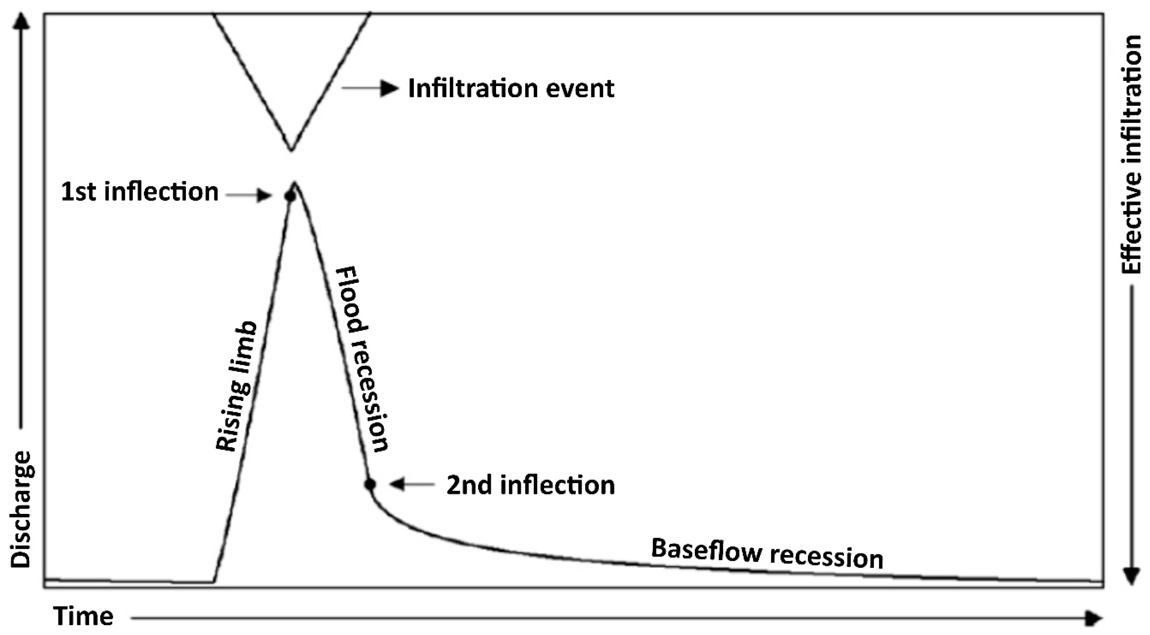
The overall response of the aquifer to each precipitation event appears as individual peaks in the hydrograph curve. Each peak has an ascending and a descending limb (Figure 1). The spring hydrograph recession curve runs from one peak to the start of the following ascending limb [11]. The falling segment is more stable than the rising part of the hydrograph and can express the hydraulic and geometric properties of the karst aquifer [12]. The descending limb of the hydrograph includes at least two parts with steep (i.e., flood recession) and mild (i.e., baseflow recession) slopes.
Fiorillo [12] provides a review of the several mathematical functions that have been suggested to characterize the recession limb. The spring hydrograph is affected by a wide variety of factors, such as flow regime [14], epikarst and unsaturated zone structure [15], type of recharge [11,16], amount of annual precipitation [16], frequency of precipitation events, the shape and size of catchment area [11], geometry and hydraulic properties of conduits [5,11], transfer flow between conduit and matrix [17], lithological characteristics of the aquifer [18], the thickness of the aquifer below the outlet [19], and the dominant conduit network pattern [20]. However, the effect of conduit network geometry on the hydrograph of springs and observation wells has not been well studied and requires more comprehensive research. This present study attempted to investigate the effect of a few frequent karst conduit patterns and how they are connected to the spring hydrograph.
The most comprehensive classification of karst conduit patterns in carbonate rocks was suggested by Palmer [21] based on the interaction between the dominant initial porosity and the type/origin of the dissolution agent (Figure 2). Among the studied caves, the branch pattern with 57% frequency and network pattern with 17% are more frequent. In the branch type, the first-order branches (i.e., order 1) are fed by a separate recharge source. The second-order branches are formed when the branches with order 1 connect to each other. With increasing the order of conduits, the groundwater flow is concentrated downstream until drained through spring. In a well-developed branchwork conduit pattern, the number of conduits (i.e., the density of conduits) tends to decrease from the upstream to the discharge site but their diameter increases. This pattern is equivalent to dendritic river channels with rarely closed loops. Contrary to the branching pattern, closed loops are abundant in the network pattern, and it has a similar appearance to the streets of a city [21]. Since the map of actual conduit patterns is rarely known except by direct cave mapping and/or partly by indirect geophysical methods, a wide range of theoretical approaches has been introduced to generate the possible karst conduit patterns [22,23,24].
Several methods have been proposed to generate a pattern of possible karst conduits, which in general, can be said to follow two approaches: structure-imitating and process-imitating. Reproducing the network of conduit structure by statistical methods that are not reliant on calculations from physical and chemical processes is the aim of structural imitation approaches [24,26,27,28]. How to generate realistic connection patterns using pure statistical tools is still an open question. On the contrary, the process-imitating approach attempted to produce a pattern of conduits based on speleogenesis principles [29,30,31]. Positive feedback between dissolution and flow leads to self-organization of the conduit network, consequently creating a realistic conduit pattern. However, the dependence of the produced conduit network on the model boundary conditions is one of the disadvantages of this approach [32,33]. To model the flow and particle transport in a hypothetical karst system, Ronayne [28] used the invasion percolation algorithm to generate a conduit network, which is an example of a structure-imitating approach. This structural model (nonlooping invasion percolation model) was suggested to produce a branch conduit pattern and cannot run for creating other conduit patterns, such as network conduit patterns [32]. The current research used a structure-based approach to generate branchwork and network maze conduit patterns.
To compare the effect of different patterns of conduit networks on the spring hydrograph, a synthetic numerical modeling approach is considered. The lack of precise data on the pattern of conduits in real-field karst aquifers causes ambiguity in the interpretation of the effect of conduit pattern on the spring hydrograph. However, a synthetic numerical modeling approach can produce a spring hydrograph under a controlled setting in a karst aquifer that is allowed to host different conduit patterns. Numerical and laboratory karst models can potentially test new hypotheses [34,35] and analyze karst aquifer’s spatial and temporal functions [34]. Despite the known challenges in applying mathematical models to karst aquifers due to the scarcity of required data, they are frequently implemented to sustain karst water resources [35]. Two general modeling approaches have been introduced in karst systems [36]: (1) spatially lumped models (i.e., global models) and (2) spatially distributed models. Two examples of lumped models are hydrograph–chemograph analysis and discharge–precipitation models [36].
Moreover, the equivalent porous medium (EPM) approach, dual porosity model (DPM), discrete fracture network approach (DFN), discrete channel network approach (DCN), and hybrid model (HM) are examples of spatially distributed models [37]. Hybrid models (HM) merge discrete (DFN and DCN) with equivalent porous medium models. These models simulate conduit and fracture as one-dimensional or two-dimensional elements in a three-dimensional matrix [36]. Insufficient knowledge of the conduit network geometry, position, distribution, and size poses significant limitations to applying numerical models in karst systems. These limitations have led to discrete–continuous numerical studies often performed on karst systems with simple conduit geometry. Yet, natural karst aquifers are typically quite heterogeneous and have complicated conduit networks. Due to the heterogeneity and influence of hydrodynamic characteristics of the aquifer, conduit networks are significant. An appropriate assessment of the state of the karst system’s conduit network should be given to improve the accuracy of the modeling of the karst system [33].
This research addresses three basic inquiries: (1) how the randomly generated network maze conduit pattern compared to the branchwork pattern, (2) how the pattern and geometry of the karst conduits (i.e., branchwork and network maze patterns) affect the characteristics of the spring hydrograph, for example, the time to reach a peak discharge and baseflow discharge and recession coefficients, and (3) how the recharge types (i.e., concentrated and diffuse) alter the conduit pattern’s impact on the spring hydrograph.
2. Methods
2.1. Generation of Conduit Networks
Two conduit patterns, branchwork and network, were generated to assess the effects of the pattern of conduits on the spring hydrograph. A series of MATLAB codes were utilized to create the patterns.
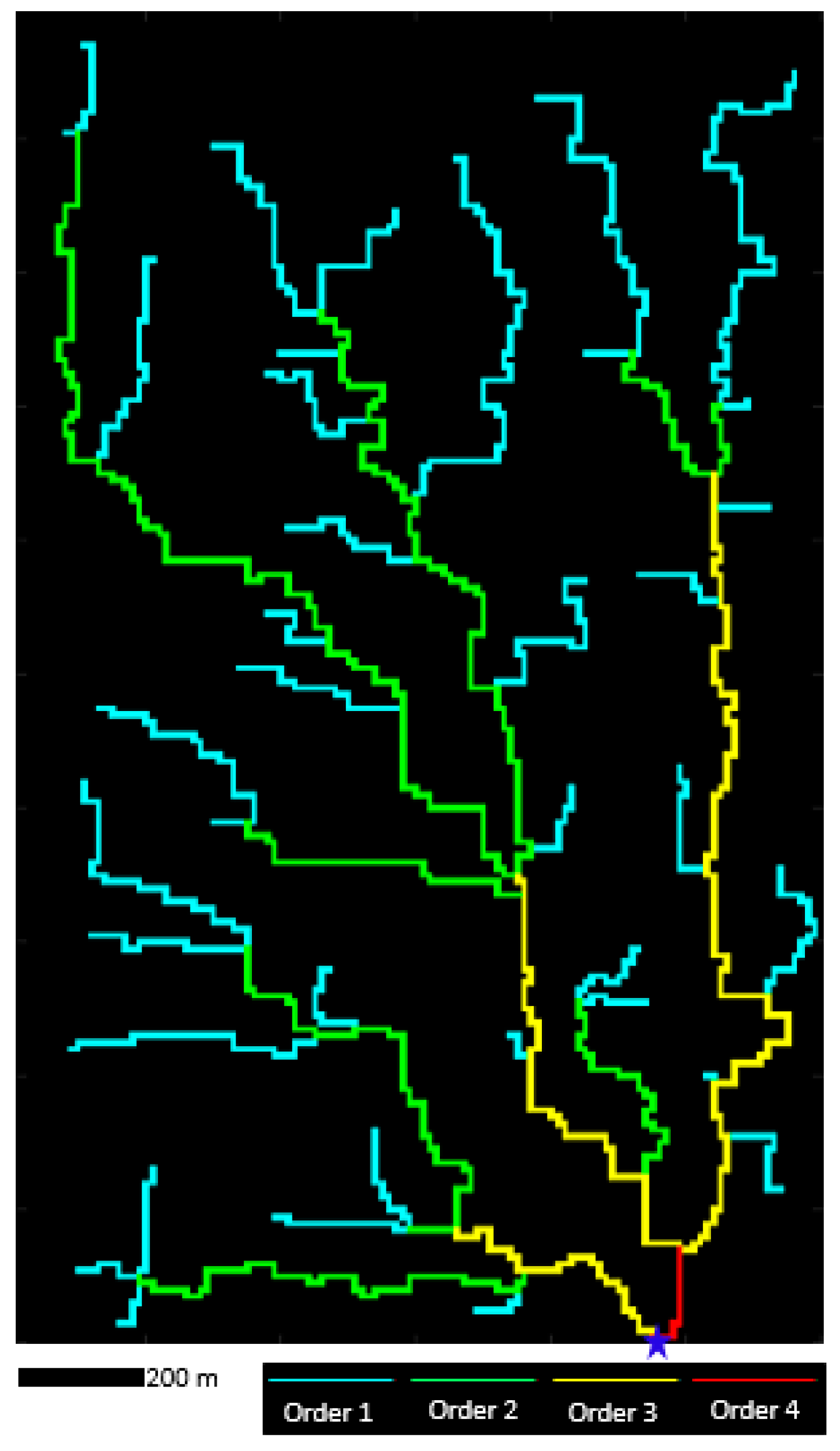
The curvilinear branchwork pattern was generated based on the MATLAB program (MATLAB code S1) introduced by Ronayne [38]. In the first step, a two-dimensional grid with normal distribution is created. Each square cell of the grid is randomly assigned a resistance value, indicating the cell’s resistance to invasion. This resistance represents the combined effect of different physical properties of the karst media, such as limestone purity, stratigraphy, tectonics, etc. In the second step, one seed cell (as a spring) is defined in the lowest row of the grid area (i.e., lower boundary). In the third step, the conduit growth starts from the seed location and continues by attacking the neighboring cells with the least resistance. A maximum of two neighboring cells can be attacked in each iteration. The newest conduit cells attacked at one growth stage are considered the source cells at the next stage. To prevent loops in the conduit network, the new cell is only attacked if all its neighbors except the source cell are not occupied. The conduit network continues to expand in this manner until there are no more sites to attack; usually, this happens when the conduit network reaches the boundary of the area (right, left, and upper boundary of the grid domain). In the fourth step, a number is assigned to the tributaries of the conduit network based on the ordering method proposed by Strahler [39]. Finally, all tributaries of the conduit network are numbered from order 1 to the largest order, which is allocated to the tributaries far from and close to the spring, respectively (Figure 3). The curvilinear branchwork pattern may be generated with different geometry in terms of length, density, tortuosity, and direction of tributaries by changing the anisotropy factor and assuming a threshold for the order of conduits [28].
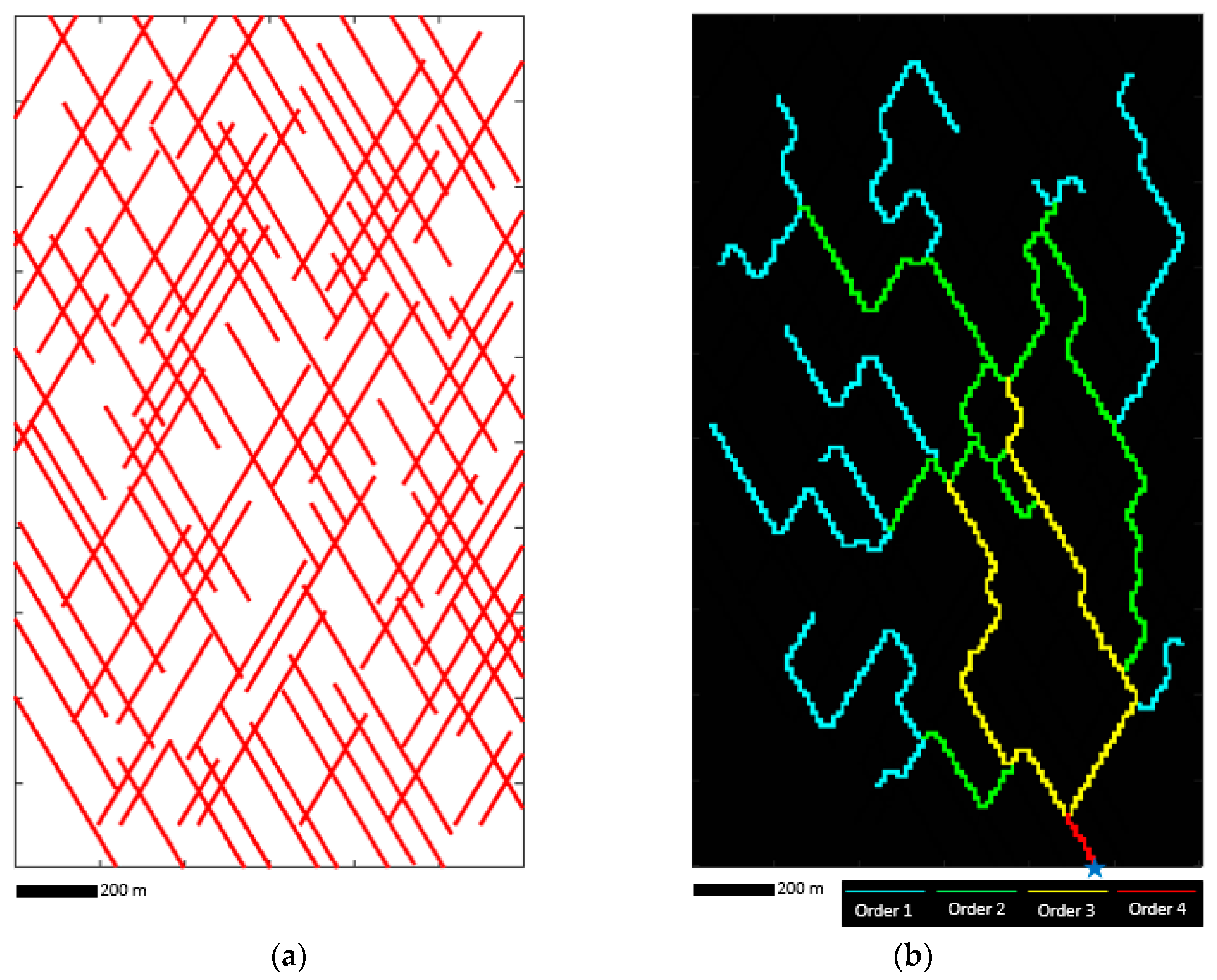
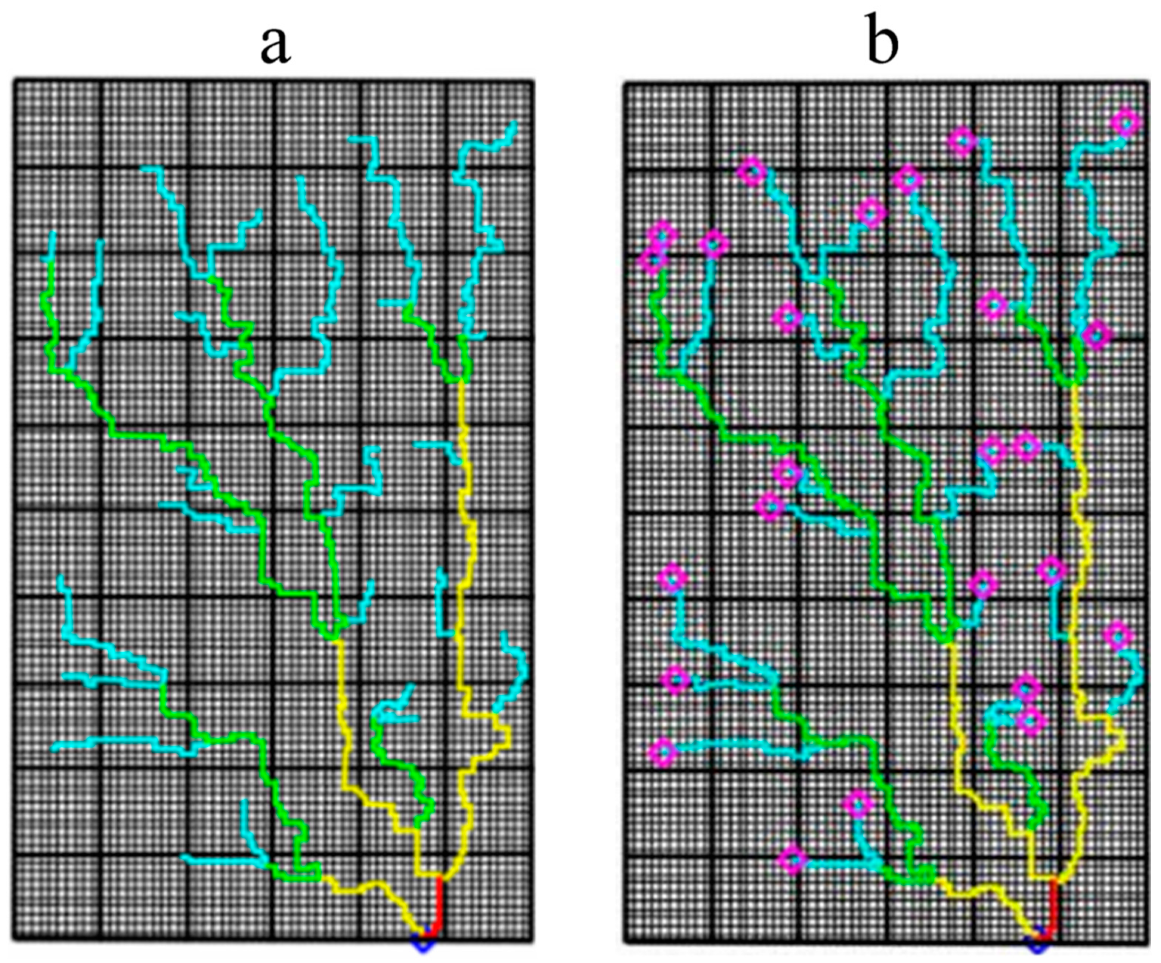
A network conduit pattern (Figure 4b) was generated with the following steps: (1) a two-dimensional joint set (Figure 4a) was randomly generated using the ADFNE1.5 code (MATLAB code S2) [40], and (2) one seed cell (as a spring) is defined in the lower boundary, and the conduit growth starts from the seed location and continues along the joints. The neighbors that can be attacked are a maximum of three; for a new cell to be attacked, its neighbors do not need to be unoccupied. Such conditions enable the formation of loops in the conduit network because a cell can be attacked from different paths. Where the conduit network’s growth reaches the joint intersection, it continues in shorter paths first, and (3) the conduit network was ranked using the algorithm proposed by Gleyzer et al. [41]. This algorithm allows a conduit to split into several downstream conduits, which can be reconnected at one point. The loops with the greatest distance from the starting point of the network (seed cell) are ranked first, and the order of conduits increases if independent tributaries join together [41].
The generation of the rectilinear branchwork pattern is similar to the network maze pattern (MATLAB code S3), but the creation of closed loops in the conduit network is prevented.
2.2. Conceptual Model and Model Description
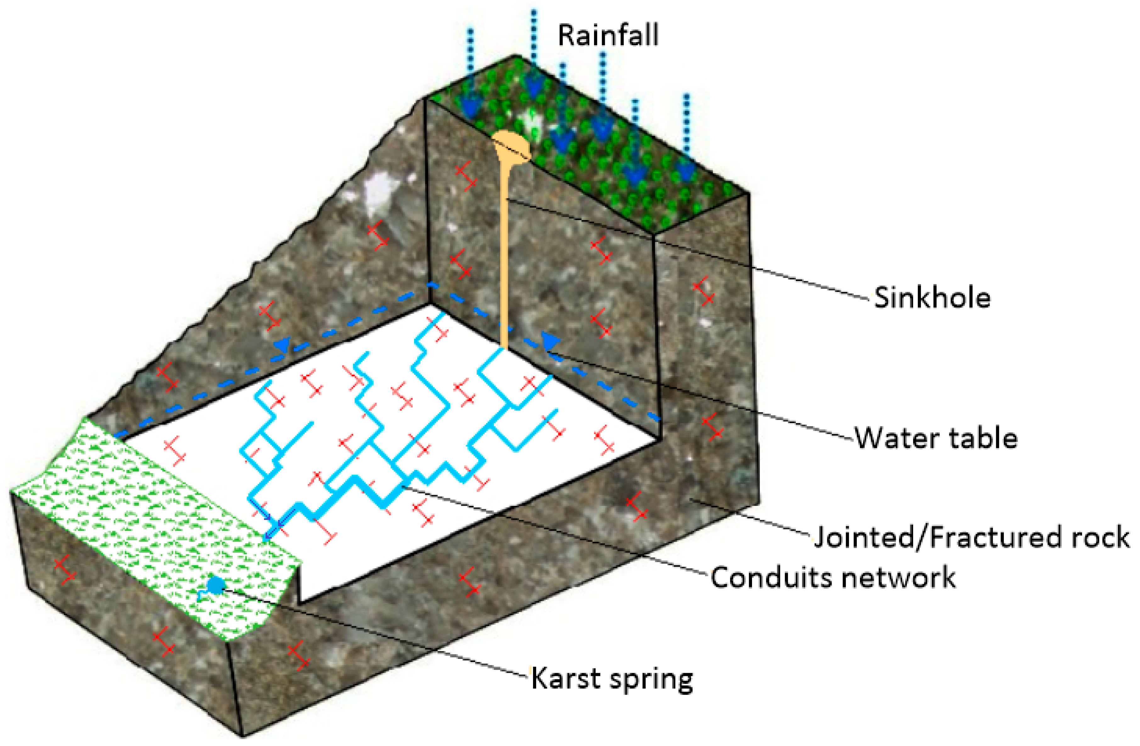
A conceptual model was created based on a synthetic karst aquifer to evaluate the impact of the conduit pattern on the karst spring hydrograph (Figure 5). Hypothetical karst conduits (i.e., generated branchwork and network patterns in Section 2.1) were transferred to ModelMuse v.4.2, and their hydrogeological parameters were defined. ModelMuse is an intuitive software package for running groundwater models, such as MODFLOW–2005, MODFLOW–CFP, etc. [42]. MODFLOW-CFP is a hybrid model that simulates flow in a karst aquifer with three modes. CFP-Mode1 simulates the behavior of dual porosity in karst aquifers by coupling a linear flow model (MODFLOW-2005) with a network of discrete tubes/pipes (conduit system) [43]. MODFLOW-CFP employs the block-centered formulation, in which a node exists in each cell and is responsible for calculating the hydraulic head [43]. Each conduit is defined by a pipe that connects two nodes (the length of each pipe is equal to the distance between two nodes). Input parameters in CFP-Mode1 include pipe height, pipe diameter, tortuosity, roughness coefficient, pipe wall permeability (exchange coefficient between pipe and matrix), and the upper and lower limit of Reynolds number.
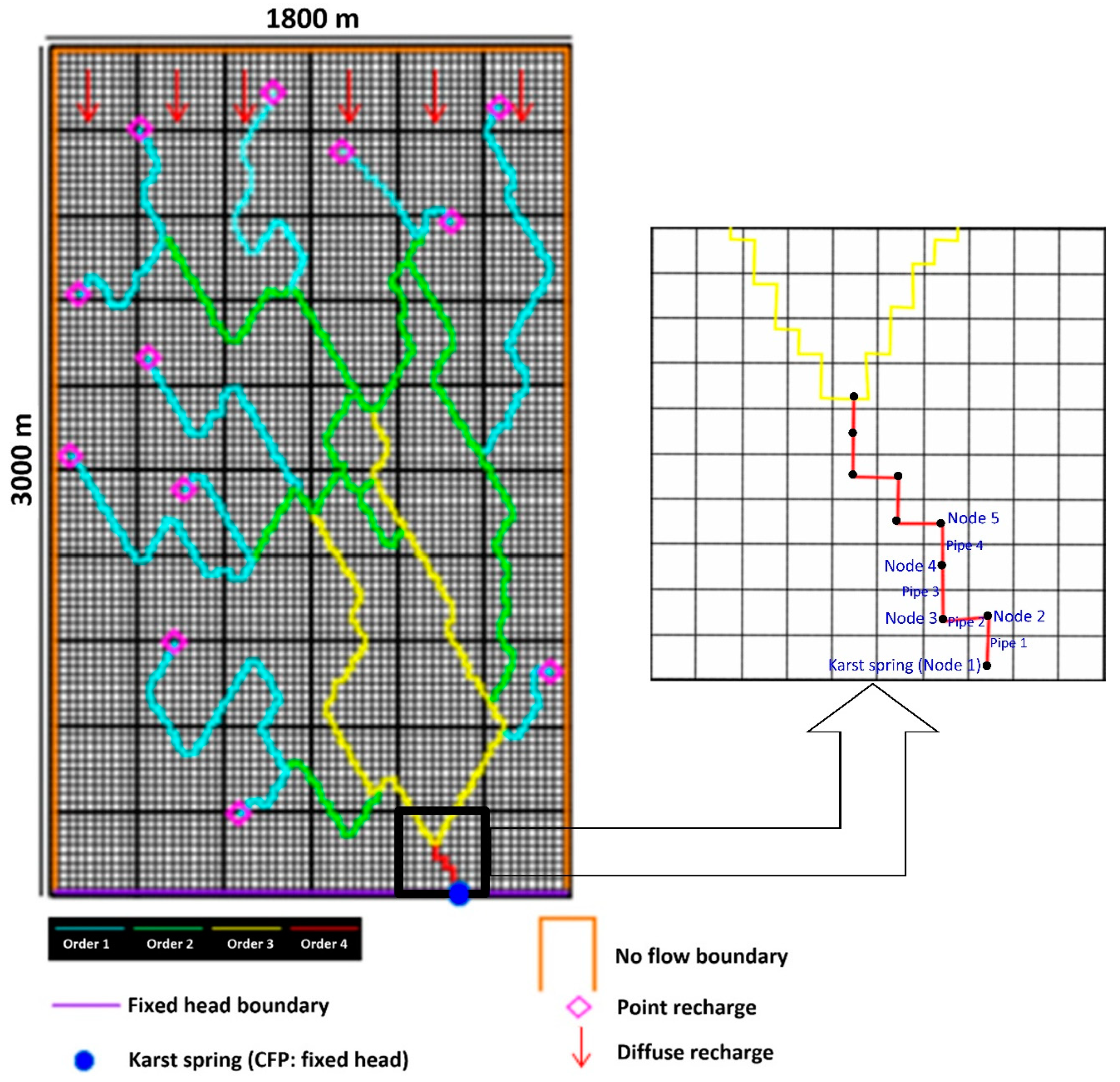
The synthetic karst aquifer includes the conduit network hosted by a low permeability matrix, as assumed in previous studies (Chang et al. [5], Reimann and Hill [35], and Reimann et al. [44]). The matrix/fissured and conduit systems are coupled to represent the hydraulic system [45]. The model domain extends over 3000 × 1800 m, which is divided into cells with a length and width of 10 m. The synthetic karst aquifer was assumed to be an unconfined aquifer with a thickness of 400 m, and an elevation of zero was assigned to the bottom of the aquifer. The matrix is considered a homogeneous media with hydraulic conductivity and a specific yield of m/s, and , respectively. The conduit wall permeability (i.e., k-exchange) was assumed to be m/s. A karst spring with an elevation of 60 m was treated as the fixed head boundary. The initial head of the matrix was set to 60 m. Moreover, an elevation of 50 m was assigned to the elevation of conduits. The boundaries around the model were considered as no flow and fixed head boundaries (Figure 6).
Figure 5.
Schematic presentation of the synthetic karst aquifer (modified from Hubinger and Birk [46]).
Figure 5.
Schematic presentation of the synthetic karst aquifer (modified from Hubinger and Birk [46]).

The conduit networks include 774 nodes and 773 pipes, which are classified into 4 orders of diameter. The conduit Node 1 was set to a fixed head boundary representing a karst spring (Figure 6). To assign a reliable diameter to the conduits, conceptual and physical processes in developing different conduit patterns are considered. In particular, we know that the curvilinear branchwork pattern is generally developed along the bedding planes with dominant point recharge. In contrast, the rectilinear branchwork pattern combines joint and fracture structures and point recharge conditions [25]. However, the porosity of joints and fractures under diffuse recharge is responsible for developing a network maze conduit pattern. Therefore, since a uniform recharge through joints and fractures causes similar karst development in the network maze conduit pattern, the diameters of the conduits are assumed to be equal in the whole flow domain (Table 1). However, conduits enlarge hierarchically in the branchwork pattern. The conduit’s diameter tends to be larger, close to the discharging spring, compared to the recharge area far from the spring location [25]. The assumed specifications (i.e., order and diameter) for the three patterns of conduit are shown in Table 1.
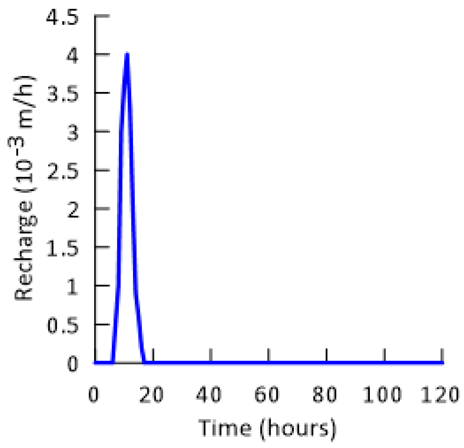
The entire model domain is supplied with constant diffuse recharge of m/h. Additionally, the diffuse recharge caused by a multi-hour precipitation event was applied to all model cells (Figure 7). Moreover, in a few scenarios (Section 2.3), part of recharge is applied directly to the conduits through sinkholes as point recharge.
2.3. Simulation Scenarios
In order to assess the effect of conduit network geometry (e.g., curvilinear and rectilinear branchwork patterns versus network maze pattern), conduit density, and recharge type (e.g., diffuse versus point recharge) on the spring hydrograph, three sets of scenarios were considered (Table 2).
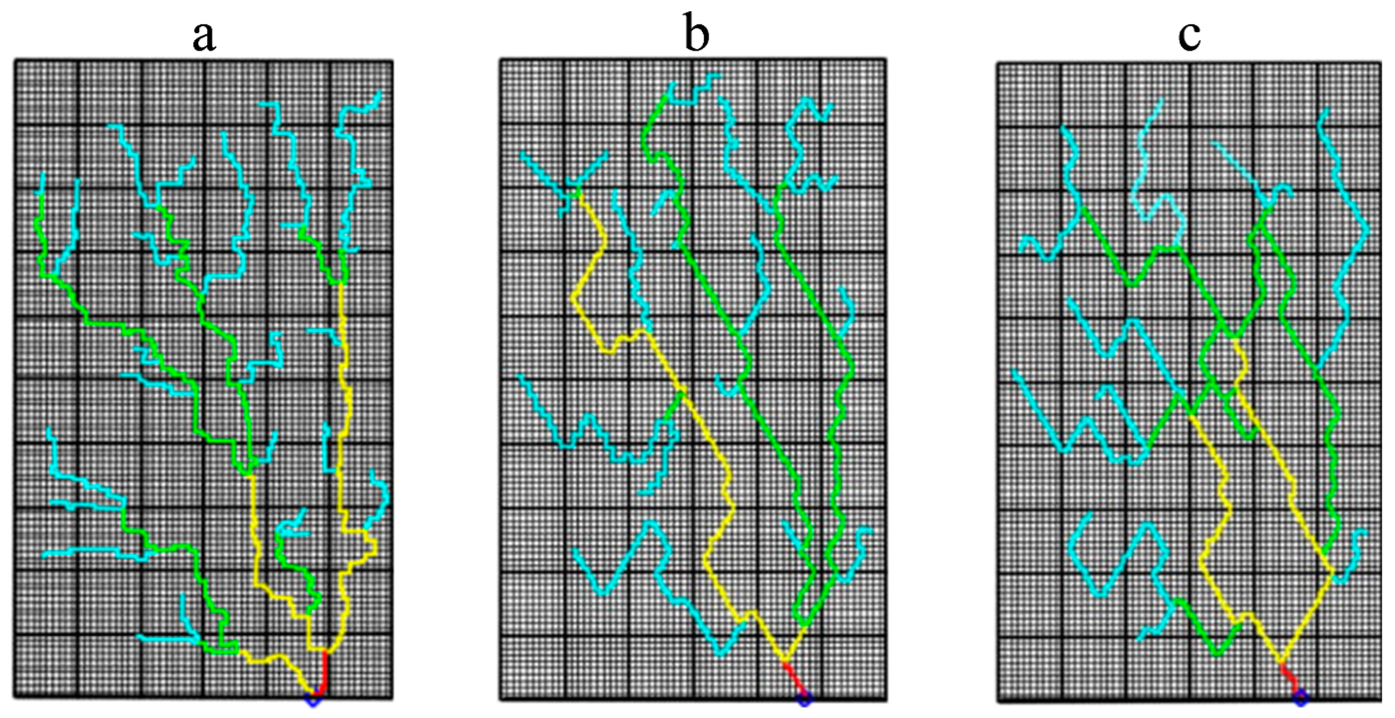
The conduit pattern is the only variable assessed in scenario A (CFP input files S1). Other variables include hydrogeological characteristics of the aquifer (K, T, and S), exchange coefficient between matrix and conduits (K-exchange), the volume of conduit network, boundary conditions (no flow boundary, fixed head boundary, karst spring), and the type of recharge are the same in the three models of the scenario A (Table 2). The diffuse recharge type is considered in scenario A, and none of the conduit nodes receives the point recharge. Three conduit patterns (i.e., curvilinear branchwork, rectangular branchwork, and network maze) were used in scenario A to compare their effect on the spring hydrograph (Figure 8).
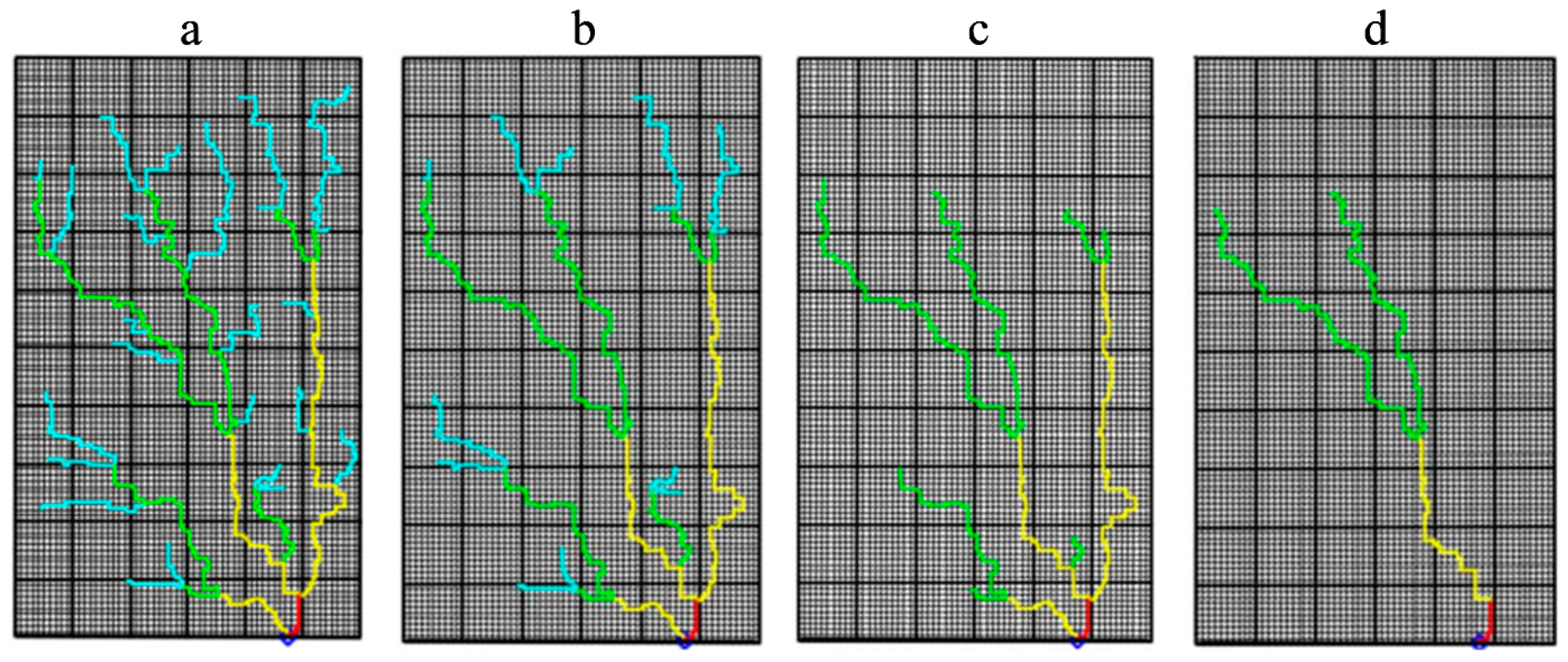
Scenario B evaluated the effect of conduit density on the spring hydrograph based on stepwise reduction of the number of conduits in three models introduced in scenario A (CFP input files S2). Therefore, for each pattern of conduits (i.e., three models in scenario A in Figure 8), three models were generated based on the reduction of conduit length by 25%, 50%, and 75% compared to the original model in Figure 8. The assumed density of conduits in curvilinear branchwork, rectangular branchwork, and network maze patterns are presented in Figure 9, Figures S1 and S2, respectively. Except for the volume of the conduits, all scenario B variables remained the same as in scenario A (Table 2). Moreover, the type and amount of recharge in scenario B are similar to scenario A.
In scenario C, the effect of recharge type (i.e., the contribution of the diffuse and point recharge) on the spring hydrograph was investigated (CFP input files S3). Three conduit patterns introduced in scenario A (Figure 8) were considered to compare the effect of stepwise reduction of the diffuse recharge by 25% and 50% and allocating these values to the point recharge. However, the rest of the variables and conditions of scenario C models remain the same as scenario A (Table 2). The pattern of conduits and the assumed location of point recharge (i.e., sinkholes) in scenario C is presented in Figure 10 and Figure S3.
3. Results and Discussion
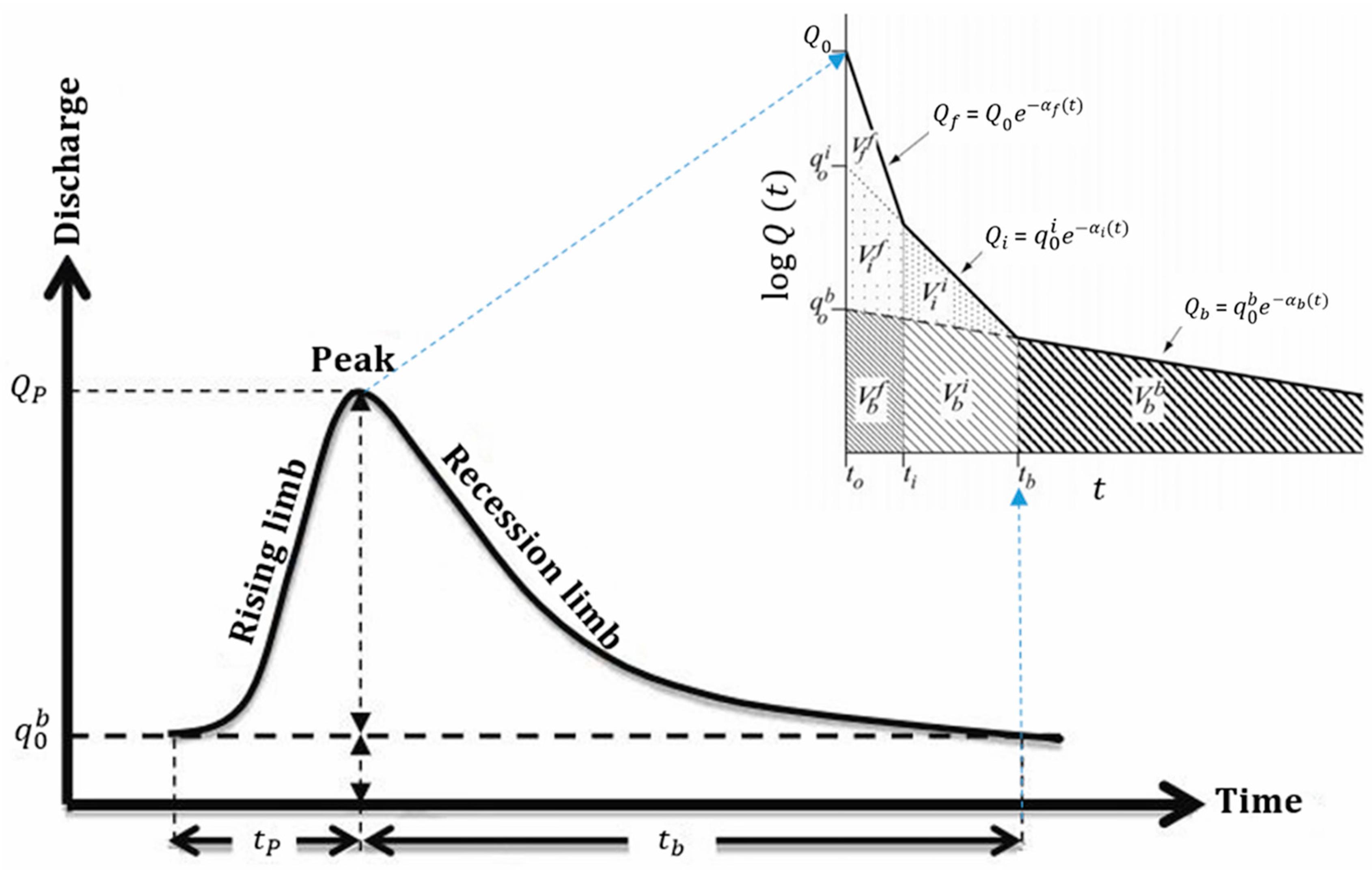
To compare the hydrographs obtained from modeling in each scenario, the parameters of peak discharge , the lag time between the peaks of recharge and discharge , baseflow discharge , the return time to baseflow discharge , the fast-flow recession coefficient , the intermediate recession coefficient , the baseflow recession coefficient , the fast flow volume , the intermediate flow volume , and the baseflow volume from the spring hydrograph curve were extracted and evaluated (Figure 11).
The entire discharge–time relationship of the recession and the total volume of water drained across the recession from to is expressed based on Equations (1) and (2), respectively [47,48].
![Water 15 01594 g011]()
Figure 11.
Schematic representation of karst spring hydrograph [49] and recession curve [47]. is the peak discharge of spring, is the base discharge, is the time duration to reach the peak discharge, and represents the return time from the peak discharge to the baseflow. In the recession curve, or is the flow rate, is the discharge volume, is the recession coefficient, and is time. Index indicative beginning points, and indices of , and are the abbreviation of fast, intermediate, and baseflow, respectively.

Although just two types of hydraulic conductivity and storativity (matrix and conduits) were considered in the synthetic karst aquifer, the recession curve can show multiple segments with different recession coefficients in the semilogarithmic plot. Kira’ly and Morel [50] and Eisenlohr et al. [11] attributed the appearance of the intermediate exponential section to transient phenomena near the conduit network with high hydraulic conductivity.
Each recession segment has also been explained as the drainage of sinkholes, the first, and drainage of the saturated zone, the following, under different hydraulic laws [51,52].
3.1. The Effect of the Conduit Pattern
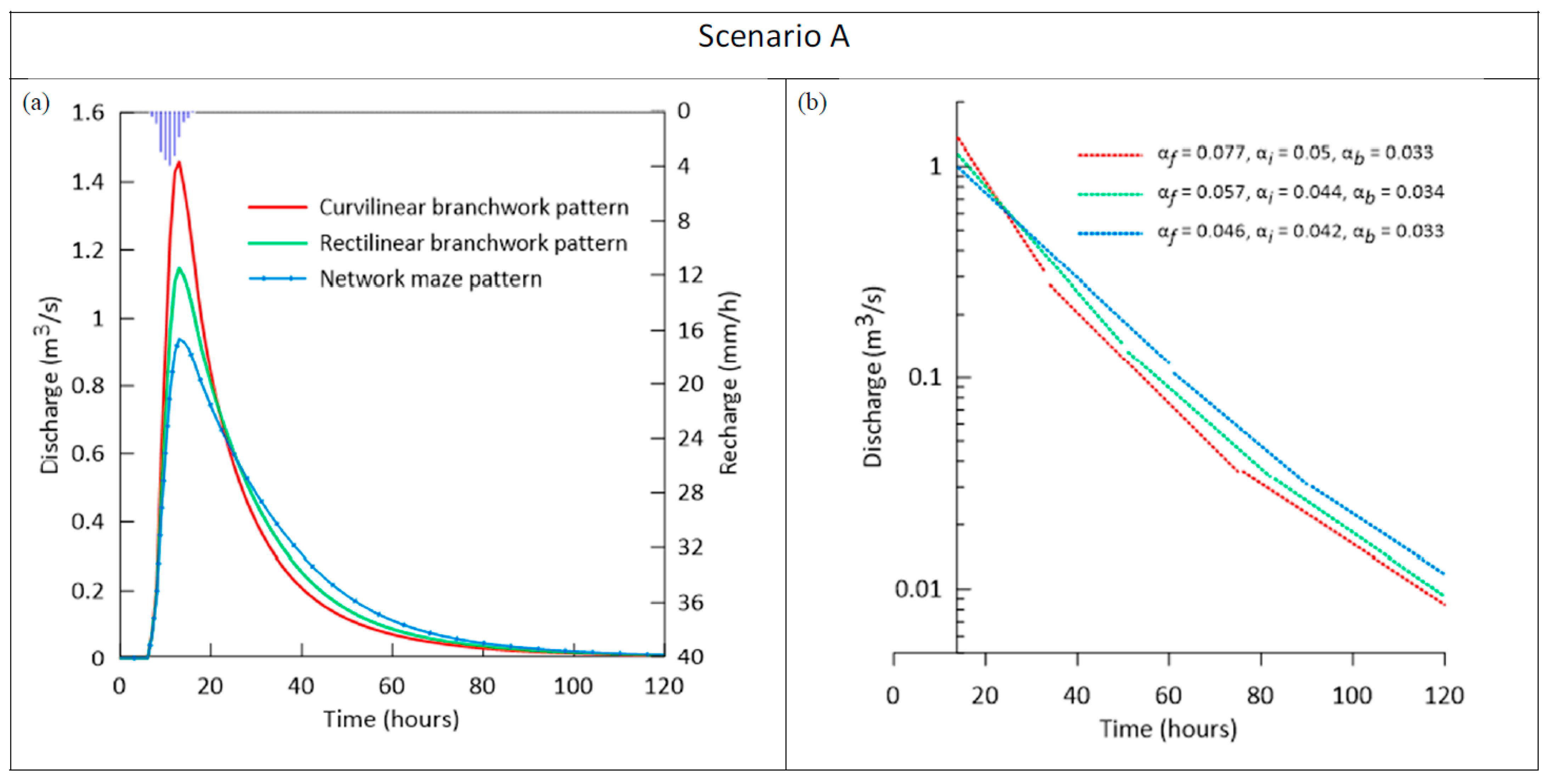
In order to assess the effect of conduit patterns in scenario A, three models that differ only in their conduit patterns are compared. The modeling results show that changes under the influence of the pattern of conduits. The increase in is attributed to the relatively larger diameter of the conduits close to the spring and the higher degree of conduit connections in the branchwork patterns compared to the network pattern. Since the rising limb of the hydrograph curve is more affected by the recharge condition [53,54], and in scenario A, the type and amount of recharge was assumed to be the same for all three models, is similar for different patterns of conduits (Figure 12 and Figure 13; Table S1). However, and are different in the three models, indicating the slower water transfer in the maze pattern than in the branched patterns (Figure 12 and Figure 13; Table S1).
Although the recession coefficient depends on a reservoir’s permeability, storage, and geometric properties [55], scenario A was designed to assess the effect of conduit pattern only. Since represents the most rapid drainage of the karst network by the largest conduits [47], a larger value of 0.077 is estimated for the branchwork conduit pattern compared to 0.046 in the network pattern. However, is almost similar in three assumed conduit patterns (Figure 12b and Figure 13; Table S1). Assigning similar aquifer characteristics (such as aquifer shape, hydraulic conductivity, storage coefficient, and boundary conditions) for models in scenario A caused similar for three models. Theoretically, the baseflow recession coefficient () depends on not only the hydraulic properties of the low hydraulic conductivity volumes but also the area and form of the whole aquifer geometry, the hydraulic conductivity, and the density of the conduit network with high hydraulic conductivity [11]. Results of scenario A suggest no considerable effect of the conduit patterns on .
Comparison of the percentage of volume drained by fast flow, intermediate flow, and baseflow to the total initial volume (/, /, /) revealed a larger and smaller in branchwork patterns related to the network pattern. In the network maze pattern, / is less than the branching patterns, while / is higher. This means the geometry and pattern of conduits influence water transfer in the karst aquifer (Figure 13 and Table S1).
3.2. The Effect of the Conduit Density
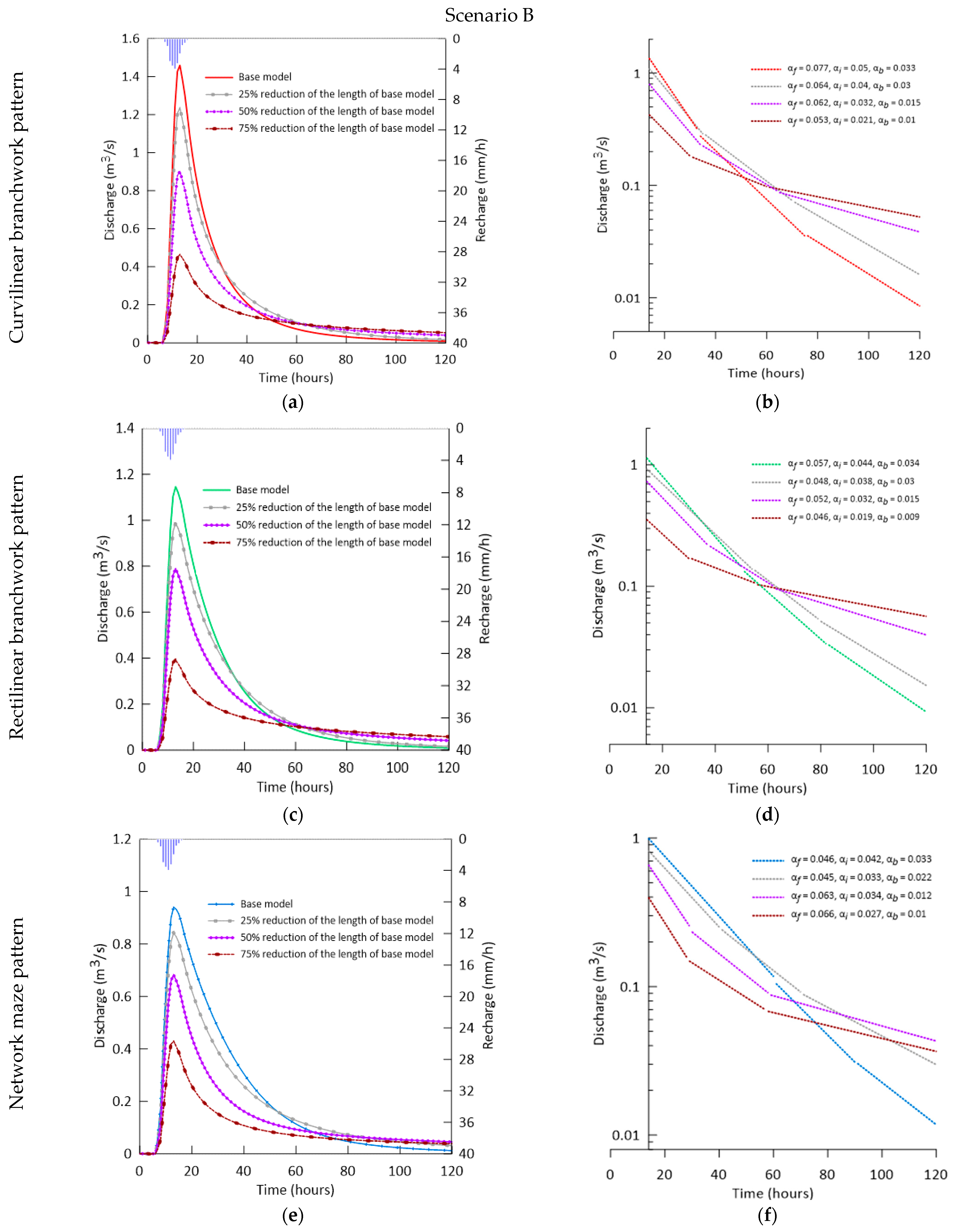
Scenario B includes nine models to examine the conduit density effect on the spring hydrograph characteristics. The scenario B model results, which assume a stepwise reduction in conduit density, revealed that decreased with decreasing density of the conduit network compared to the base model (Figure 14 and Figure 15; Table S2). The result suggests a direct relationship between the length of the conduit network and the amount of spring discharge. The greater conduit density (i.e., the total length of the conduit network) causes a higher water transfer rate and, consequently, a more significant peak discharge. In scenario B, is similar in all models due to assuming similar recharge conditions in all models (Figure 14 and Figure 15; Table S2).
Generally, decreasing the density of the conduit network reduced the values of , , and due to the reduction in conduit volume and the slow transfer of water from the matrix to the conduits. There are a few exceptions that seem to be affected by the reverse exchange of water between the conduits and matrix (Figure 14b,d,f and Figure 15; Table S2).
In all models implemented in Scenario B, the baseflow recession coefficient has decreased with decreasing conduit network density. Since the other factors affecting the value of (hydraulic properties of the matrix, area and form of the whole aquifer, and the hydraulic conductivity of conduits) remain constant in all models; the simulation results prove the effect of conduit network density and geometry on . Results elucidate that the percentage of volume drained by fast flow, intermediate flow, and baseflow to the total initial volume correlates to the proportion to the density of the conduit network. In particular, decreasing the density of conduits causes a decreasing and increasing trend in / and /, respectively (Figure 14b,d,f and Figure 15; Table S2).
3.3. The Effect of Recharge Type
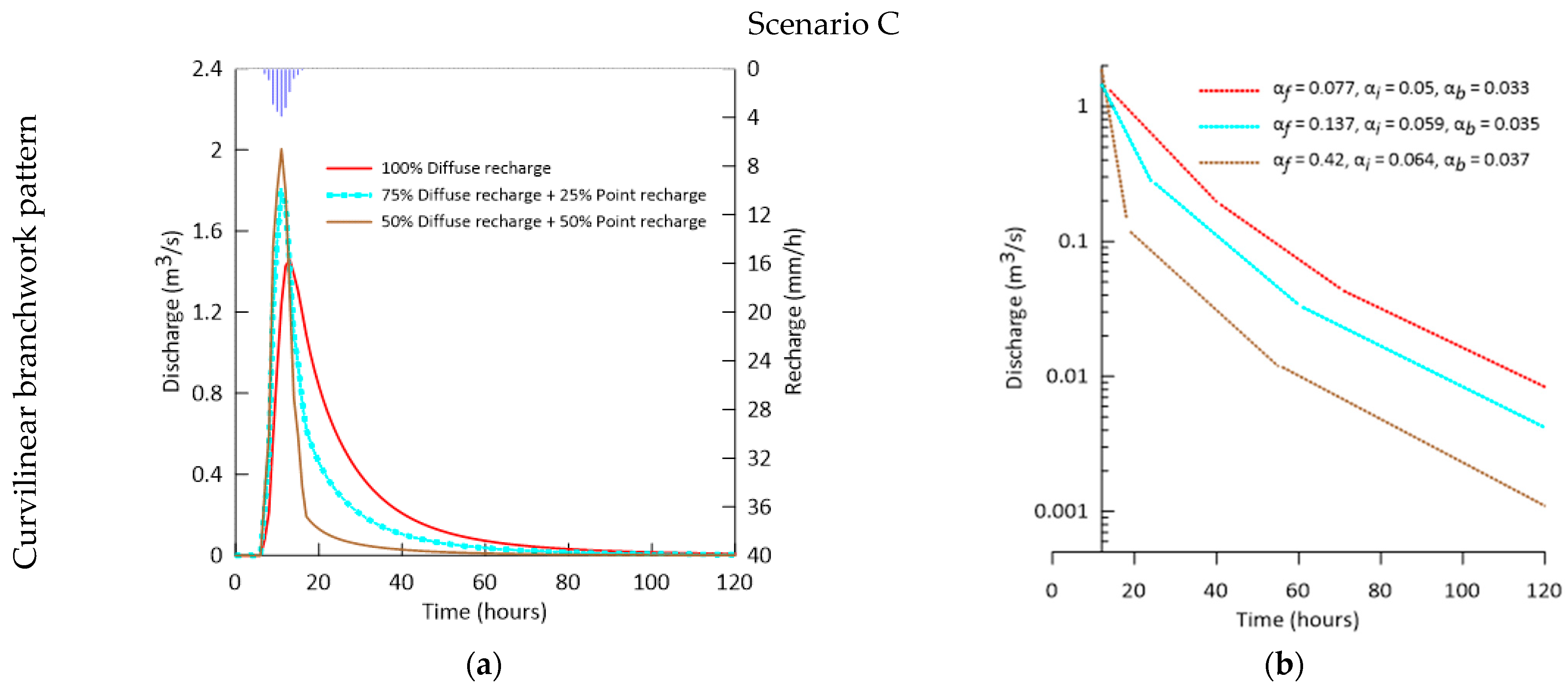
Different contributions of point and diffuse recharge in six scenario C models were assumed to assess the effect of recharge type on the characteristics of the spring hydrograph. The results of scenario C indicate that an increased proportion of point recharge compared to diffuse recharge decreases and (Figure 16 and Figure 17; Table S3). Moreover, increasing the role of point recharge increased and decreased and , respectively, in three patterns of conduits (Figure 17 and Table S3), as mentioned by Kovács and Perrochet [56].
Values of increase with increasing point recharge ratio but values do not noticeably change, except in one case (Figure 16b,d,f and Figure 17; Table S3). Based on investigations by Kovács and Perrochet [56] and Kovács et al. [55], is exclusively dependent on the hydraulic characteristics of the matrix and the total extent of the aquifer; thus, a different proportion between concentrated and diffuse recharge does not influence the value of . However, in the presence of point recharge, if the diameter of conduits is not large enough to quickly transfer the recharge water, the excess volume of water could enter the matrix and affects the and . It is also possible that the conduit network connections in response to a point recharge or diffuse recharge play a different role and influence the baseflow recession that needs more research under different hydraulic conditions.
4. Field Examples to Verify the Results
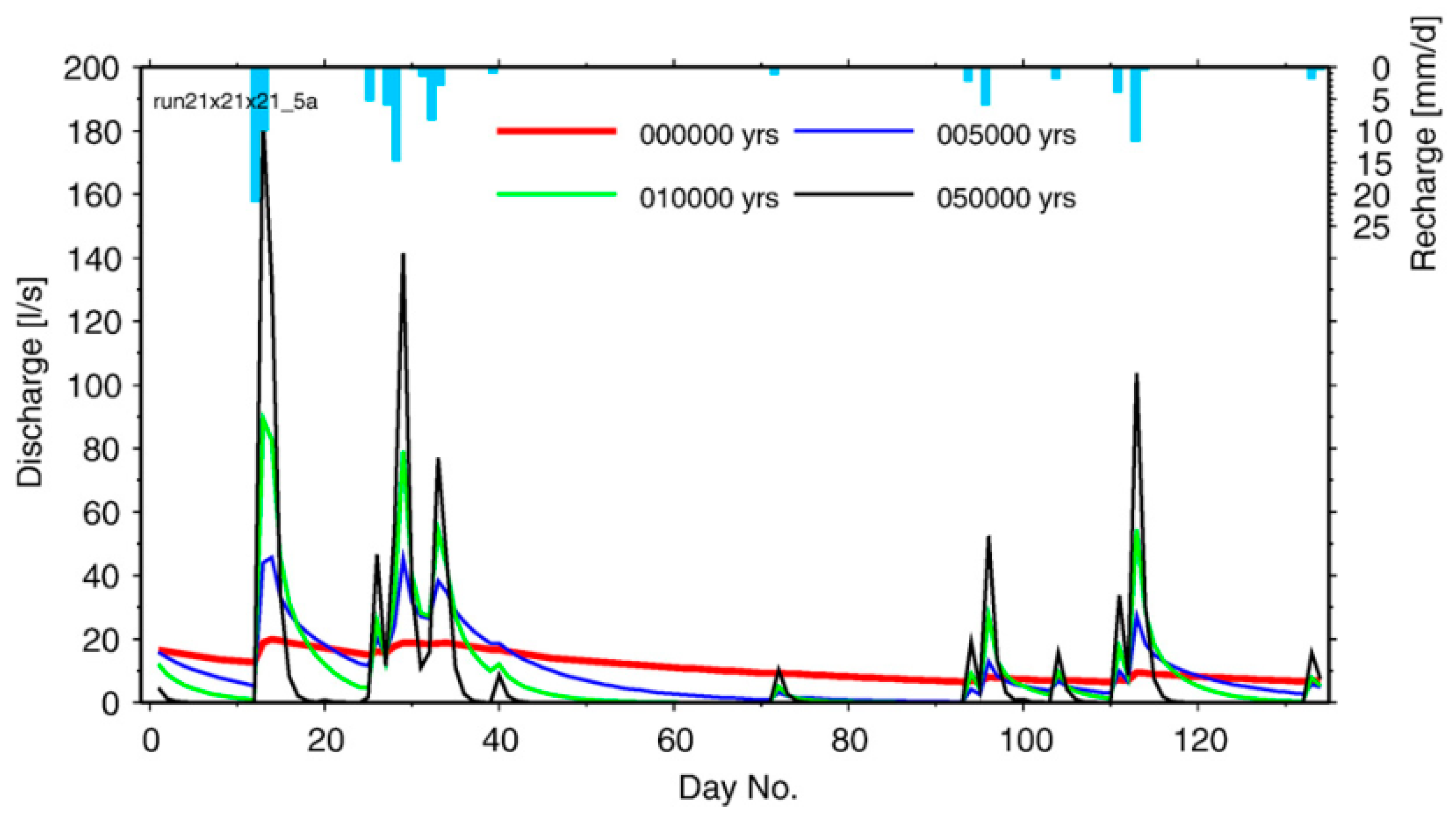
Understanding the relationship between springs and conduit patterns is vital in groundwater resource management of karst systems because it contributes to delineating both the area of recharge that contributes to spring flow and the potential for rapid groundwater/surface water exchange [57]. Kaufmann [58] studied flow evolution in a karst aquifer by numerical simulation based on chemical dissolution over time to enlarge fractures and generate the conduit network. The results of this study have shown that the response of karst spring changes based on the development of conduit patterns (Figure 18). The graphs in Figure 18, which are the results of a simulation of the development of karst conduits, show that as more time passes and the length and size of the conduits increase, the shape of the spring hydrograph changes significantly. Somehow, this conclusion confirms the results of scenario B, which investigates the effect of conduit network density on the shape of the spring hydrograph.
According to the length of mapped conduits, Wakulla–Leon Sinks Cave System (51,484 m) and Sally Ward Cave (2090 m) are 2 of the largest mapped caves in the Woodville Karst Plain (WKP). In the WKP, the dissolution process leads to dendritic (branchwork pattern) cave systems that originate from large single conduits at springs, towards the upstream of the basin, and away from the springs; they are divided into numerous and smaller conduits [59]. Hydrographs of Wakulla and Sally Ward Springs show that both springs have a similar flow pattern [60]. Since the pattern of conduits connected to Wakulla and Sally Ward Springs and other hydrogeological conditions are alike, the difference in peak discharge, baseflow discharge, and other hydrograph characteristics can be attributed to the difference in conduit network density (i.e., similar to scenario B). The length of mapped conduits of Wakulla Cave and Sally Ward Cave is approximately 10 and 1.2 miles, respectively [61,62].
Measured and simulated spring discharge for Oje de Agua and Oje de Guillo springs are plotted versus the average amount of rain that has fallen each day at the Manati rain gauge station over 33 months (Figure 19). The Oje de Guillo spring responds more strongly (more sudden and sharper) to severe short-term rainfall events (e.g., 11/93 and 8/95) than the Oje de Agua spring. Its baseflow, which ranges from 1500 to 3000 m3/d, is much lower than the Oje de Agua spring (5000–10,000 m3/d). The recession limb of this spring has a much steeper slope compared to Oje de Agua spring, denoting a relatively short residence time in the conduit network [3,63]. Although Rodriguez-Martinez [63] classified Oje de Agua spring and Oje de Guillo spring as diffuse-type and conduit-type springs, respectively, Ghasemizadeh et al. [3] believe that conduits feed both springs. The discrepancies in their responses are mostly due to the recharge differential, with the Ojo de Guillo spring having a greater share of concentrated recharge at sinkholes and dolines. These conclusions are based on the results of scenario C.
5. Conclusions
The influence of conduit pattern, conduit density, and recharge type on the spring hydrograph in a synthetic karst aquifer was investigated. The simulation results revealed that ,, , and are mainly affected by the conduit network pattern, conduit network density, and recharge type, respectively. Larger values of and , and smaller values of , belongs to scenarios with higher conduit density, branchwork conduit patterns, and greater point recharge rates. Branchwork patterns, the lower density of the conduit network, and the increasing proportion of point recharge are mainly responsible for the reduction of .
Results suggest no influence of the pattern and density of the conduits on . However, in most cases, is reduced by increasing the proportion of point recharge. A comparison of results revealed that although has no significant dependency on the conduit network pattern and proportion of point recharge, it decreases with decreasing conduit network density. Moreover, / and / increased and decreased in response to branchwork patterns (compared to network maze pattern), higher density of conduit network, and increase in the proportion of point recharge, respectively. Finally, a few real field examples were reviewed to confirm the results of synthetic modeling scenarios. Despite the scarcity of suitable field data, comparing the results is promising. Although this research was a preliminary insight into the effect of conduit patterns on the spring hydrograph, it seems that further studies are required to clarify the role of conduit patterns in the hydrogeological processes of karst aquifers. The authors recommend developing subsequent modeling studies to compare the results of this research with considering the vertical zones of a typical karst aquifer and/or conducting inverse modeling to optimize the characteristics of conduit pattern based on the characteristics of spring hydrograph.
Supplementary Materials
The following supporting information can be downloaded at: https://www.mdpi.com/article/10.3390/w15081594/s1, Figure S1: Rectilinear branchwork patterns with different conduit densities in scenario B. a, b, c, and d represent the base rectilinear branchwork model, 25%, 50%, and 75% reduction in the length of conduits, respectively; Figure S2: Network maze patterns with different conduit densities in scenario B. a, b, c, and d represent the base network maze model, 25%, 50%, and 75% reduction in the length of conduits, respectively; Figure S3: The conduit patterns (a, b: rectilinear branchwork; c and d: network maze) used in scenario C. Models b and d run under two different modes of the point recharge. The purple squares represent the location of point recharge as sinkholes; Table S1: The characteristics of the spring hydrograph in scenario A; Table S2: The characteristics of the spring hydrograph in scenario B; Table S3: The characteristics of the spring hydrograph in scenario C.
Author Contributions
Methodology, H.O. and Z.M.; Software, H.O.; Validation, Z.M. and F.F.; Formal analysis, H.O.; Writing—original draft, H.O.; Writing—review & editing, Z.M. and F.F.; Supervision, Z.M. All authors have read and agreed to the published version of the manuscript.
Funding
The first and second authors would like to acknowledge the support from the Iran National Science Foundation (INSF) [Grant Number: 4012713] and Shiraz University.
Data Availability Statement
The data presented in this study are available in the article and supplementary material.
Conflicts of Interest
The authors declare no conflict of interest.
References
- Ford, D.; Williams, P.D. Karst Hydrogeology and Geomorphology; John Wiley & Sons: Hoboken, NJ, USA, 2007; ISBN 0-470-84997-5. [Google Scholar]
- White, W.B. Geomorphology and Hydrology of Karst Terrains; Oxford University Press: Oxford, UK, 1988. [Google Scholar]
- Ghasemizadeh, R.; Yu, X.; Butscher, C.; Padilla, I.Y.; Alshawabkeh, A. Improved regional groundwater flow modeling using drainage features: A case study of the central northern karst aquifer system of Puerto Rico (USA). Hydrogeol. J. 2016, 24, 1463. [Google Scholar] [CrossRef] [PubMed]
- Andriani, G.F.; Parise, M. On the applicability of geomechanical models for carbonate rock masses interested by karst processes. Environ. Earth Sci. 2015, 74, 7813–7821. [Google Scholar] [CrossRef]
- Chang, Y.; Wu, J.; Liu, L. Effects of the conduit network on the spring hydrograph of the karst aquifer. J. Hydrol. 2015, 527, 517–530. [Google Scholar] [CrossRef]
- Worthington, S.R. Groundwater residence times in unconfined carbonate aquifers. J. Cave Karst Stud. 2007, 69, 94–102. [Google Scholar]
- Bakalowicz, M. Karst groundwater: A challenge for new resources. Hydrogeol. J. 2005, 13, 148–160. [Google Scholar] [CrossRef]
- Padilla, A.; Pulido-Bosch, A.; Mangin, A. Relative importance of baseflow and quickflow from hydrographs of karst spring. Groundwater 1994, 32, 267–277. [Google Scholar] [CrossRef]
- Mohammadi, Z.; Raeisi, E.; Bakalowicz, M. Method of leakage study at the karst dam site. A case study: Khersan 3 Dam, Iran. Environ. Geol. 2007, 52, 1053–1065. [Google Scholar] [CrossRef]
- Jourde, H.; Massei, N.; Mazzilli, N.; Binet, S.; Batiot-Guilhe, C.; Labat, D.; Steinmann, M.; Bailly-Comte, V.; Seidel, J.-L.; Arfib, B.; et al. SNO KARST: A French network of observatories for the multidisciplinary study of critical zone processes in karst watersheds and aquifers. Vadose Zone J. 2018, 17, 1–18. [Google Scholar] [CrossRef]
- Eisenlohr, L.; Király, L.; Bouzelboudjen, M.; Rossier, Y. Numerical simulation as a tool for checking the interpretation of karst spring hydrographs. J. Hydrol. 1997, 193, 306–315. [Google Scholar] [CrossRef]
- Fiorillo, F. The recession of spring hydrographs, focused on karst aquifers. Water Resour. Manag. 2014, 28, 1781–1805. [Google Scholar] [CrossRef]
- Kovács, A.; Perrochet, P. A quantitative approach to spring hydrograph decomposition. J. Hydrol. 2008, 352, 16–29. [Google Scholar] [CrossRef]
- Bonacci, O. Karst springs hydrographs as indicators of karst aquifers. Hydrol. Sci. J. 1993, 38, 51–62. [Google Scholar] [CrossRef]
- Kiraly, L.; Perrochet, P.; Rossier, Y. Effect of the epikarst on the hydrograph of karst springs: A numerical approach. Bull. Cent. Hydrogéol. 1995, 14, 199–220. [Google Scholar]
- Mohammadi, Z.; Shoja, A. Effect of annual rainfall amount on characteristics of karst spring hydrograph. Carbonates Evaporites 2014, 29, 279–289. [Google Scholar] [CrossRef]
- Shirafkan, M.; Mohammadi, Z.; Sivelle, V.; Labat, D. The effects of exchange flow on the Karst spring hydrograph under the different flow regimes: A synthetic modeling approach. Water 2021, 13, 1189. [Google Scholar] [CrossRef]
- Amit, H.; Lyakhovsky, V.; Katz, A.; Starinsky, A.; Burg, A. Interpretation of spring recession curves. Groundwater 2002, 40, 543–551. [Google Scholar] [CrossRef]
- Dewandel, B.; Lachassagne, P.; Bakalowicz, M.; Weng, P.; Al-Malki, A. Evaluation of aquifer thickness by analysing recession hydrographs. Application to the Oman ophiolite hard-rock aquifer. J. Hydrol. 2003, 274, 248–269. [Google Scholar] [CrossRef]
- Florea, L.J.; Vacher, H. Springflow hydrographs: Eogenetic vs. telogenetic karst. Groundwater 2006, 44, 352–361. [Google Scholar] [CrossRef]
- Palmer, A.N. Origin and morphology of limestone caves. Geol. Soc. Am. Bull. 1991, 103, 1–21. [Google Scholar] [CrossRef]
- Al-Halbouni, D.; Watson, R.A.; Holohan, E.P.; Meyer, R.; Polom, U.; Dos Santos, F.M.; Comas, X.; Alrshdan, H.; Krawczyk, C.M.; Dahm, T. Dynamics of hydrological and geomorphological processes in evaporite karst at the eastern Dead Sea–a multidisciplinary study. Hydrol. Earth Syst. Sci. 2021, 25, 3351–3395. [Google Scholar] [CrossRef]
- Jeannin, P.-Y.; Groves, C.; Häuselmann, P. Speleological investigations. Methods Karst Hydrogeol. Int. Contrib. Hydrogeol. IAH 2007, 26, 25–44. [Google Scholar]
- Pardo-Igúzquiza, E.; Dowd, P.A.; Xu, C.; Durán-Valsero, J.J. Stochastic simulation of karst conduit networks. Adv. Water Resour. 2012, 35, 141–150. [Google Scholar] [CrossRef]
- Palmer, A.N. Speleogenesis in carbonate rocks. In Evolution of Karst: From Prekarst to Cessation; Inštitut za Raziskovanje Krasa, ZRC SAZU: Ljubljana, Slovenia, 2002; pp. 43–59. [Google Scholar]
- Collon, P.; Bernasconi, D.; Vuilleumier, C.; Renard, P. Statistical metrics for the characterization of karst network geometry and topology. Geomorphology 2017, 283, 122–142. [Google Scholar] [CrossRef]
- Hendrick, M.; Renard, P. Subnetworks of percolation backbones to model karst systems around Tulum, Mexico. Front. Phys. 2016, 4, 43. [Google Scholar] [CrossRef]
- Ronayne, M.J. Influence of conduit network geometry on solute transport in karst aquifers with a permeable matrix. Adv. Water Resour. 2013, 56, 27–34. [Google Scholar] [CrossRef]
- Borghi, A.; Renard, P.; Jenni, S. A pseudo-genetic stochastic model to generate karstic networks. J. Hydrol. 2012, 414, 516–529. [Google Scholar] [CrossRef]
- Jaquet, O.; Siegel, P.; Klubertanz, G.; Benabderrhamane, H. Stochastic discrete model of karstic networks. Adv. Water Resour. 2004, 27, 751–760. [Google Scholar] [CrossRef]
- Lafare, A. Modélisation Mathématique de la Spéléogenèse: Une Approche Hybride à Partir de Réseaux de Fractures Discrets et de Simulations Hydrogéologiques. Ph.D. Thesis, Université Montpellier II, Montpellier, France, 2011. [Google Scholar]
- De Rooij, R.; Graham, W. Generation of complex karstic conduit networks with a hydrochemical model. Water Resour. Res. 2017, 53, 6993–7011. [Google Scholar] [CrossRef]
- Henson, W.R.; de Rooij, R.; Graham, W. What Makes a First-Magnitude Spring?: Global Sensitivity Analysis of a Speleogenesis Model to Gain Insight into Karst Network and Spring Genesis. Water Resour. Res. 2018, 54, 7417–7434. [Google Scholar] [CrossRef]
- Kaufmann, G.; Romanov, D.; Hiller, T. Modeling three-dimensional karst aquifer evolution using different matrix-flow contributions. J. Hydrol. 2010, 388, 241–250. [Google Scholar] [CrossRef]
- Reimann, T.; Hill, M.E. MODFLOW-CFP: A new conduit flow process for MODFLOW–2005. Groundwater 2009, 47, 321–325. [Google Scholar] [CrossRef]
- Ghasemizadeh, R.; Hellweger, F.; Butscher, C.; Padilla, I.; Vesper, D.; Field, M.; Alshawabkeh, A. Groundwater flow and transport modeling of karst aquifers, with particular reference to the North Coast Limestone aquifer system of Puerto Rico. Hydrogeol. J. 2012, 20, 1441. [Google Scholar] [CrossRef] [PubMed]
- Sauter, M.; Geyer, T.; Kovács, A.; Teutsch, G. Modellierung der hydraulik von karstgrundwasserleitern–eine übersicht. Grundwasser 2006, 11, 143–156. [Google Scholar] [CrossRef]
- Ronayne, M.J. Understanding Groundwater Dynamics in Structurally Heterogeneous Aquifers. Ph.D. Thesis, Stanford University, Stanford, CA, USA, 2008. [Google Scholar]
- Strahler, A.N. Quantitative analysis of watershed geomorphology. Eos Trans. Am. Geophys. Union 1957, 38, 913–920. [Google Scholar] [CrossRef]
- Alghalandis, Y. DFNE Practices with ADFNE; Alghalandis Computing: Toronto, ON, Canada, 2018. [Google Scholar]
- Gleyzer, A.; Denisyuk, M.; Rimmer, A.; Salingar, Y. A Fast Recursive Gis Algorithm for Computing Strahler Stream Order in Braided and Nonbraided Networks 1. JAWRA J. Am. Water Resour. Assoc. 2004, 40, 937–946. [Google Scholar] [CrossRef]
- Winston, R.B. ModelMuse Version 4: A graphical user interface for MODFLOW 6. In Scientific Investigations Report-US Geological Survey; US Department of the Interior, US Geological Survey: Reston, VA, USA, 2019. [Google Scholar]
- Shoemaker, W.B.; Kuniansky, E.L.; Birk, S.; Bauer, S.; Swain, E.D. Documentation of a Conduit Flow Process (CFP) for MODFLOW-2005; US Department of the Interior, US Geological Survey: Reston, VA, USA, 2008; Volume 6.
- Reimann, T.; Rehrl, C.; Shoemaker, W.B.; Geyer, T.; Birk, S. The significance of turbulent flow representation in single-continuum models. Water Resour. Res. 2011, 47, W09503. [Google Scholar] [CrossRef]
- Liedl, R.; Sauter, M.; Hückinghaus, D.; Clemens, T.; Teutsch, G. Simulation of the development of karst aquifers using a coupled continuum pipe flow model. Water Resour. Res. 2003, 39, 1057. [Google Scholar] [CrossRef]
- Hubinger, B.; Birk, S. Influence of initial heterogeneities and recharge limitations on the evolution of aperture distributions in carbonate aquifers. Hydrol. Earth Syst. Sci. 2011, 15, 3715–3729. [Google Scholar] [CrossRef]
- Doctor, D.H.; Alexander, E.C., Jr. Interpretation of water chemistry and stable isotope data from a karst aquifer according to flow regimes identified through hydrograph recession analysis. In US Geological Survey Karst Interest Group Proceedings, Rapid City, South Dakota; BiblioGov: Singapore, 2005; pp. 82–92. [Google Scholar]
- Jakada, H.; Chen, Z.; Luo, M.; Zhou, H.; Wang, Z.; Habib, M. Watershed characterization and hydrograph recession analysis: A comparative look at a karst vs. non-karst watershed and implications for groundwater resources in Gaolan River Basin, Southern China. Water 2019, 11, 743. [Google Scholar] [CrossRef]
- Şen, Z. General modeling of karst spring hydrographs and development of a dimensionless karstic hydrograph concept. Hydrogeol. J. 2020, 28, 549–559. [Google Scholar] [CrossRef]
- Király, L.; Morel, G. Remarques sur l’hydrogramme des sources karstiques simulé par modèles mathématiques: Avec 15 figures. Bull. Cent. Hydrogéol. 1976, 1, 37–60. [Google Scholar]
- Fiorillo, F. Tank-reservoir drainage as a simulation of the recession limb of karst spring hydrographs. Hydrogeol. J. 2011, 19, 1009. [Google Scholar] [CrossRef]
- Abirifard, M.; Birk, S.; Raeisi, E.; Sauter, M. Dynamic volume in karst aquifers: Parameters affecting the accuracy of estimates from recession analysis. J. Hydrol. 2022, 612, 128286. [Google Scholar] [CrossRef]
- Geyer, T.; Birk, S.; Liedl, R.; Sauter, M. Quantification of temporal distribution of recharge in karst systems from spring hydrographs. J. Hydrol. 2008, 348, 452–463. [Google Scholar] [CrossRef]
- Kovács, A.; Perrochet, P.; Darabos, E.; Lénárt, L.; Szűcs, P. Well hydrograph analysis for the characterisation of flow dynamics and conduit network geometry in a karst aquifer, Bükk Mountains, Hungary. J. Hydrol. 2015, 530, 484–499. [Google Scholar] [CrossRef]
- Kovács, A.; Perrochet, P.; Király, L.; Jeannin, P.-Y. A quantitative method for the characterisation of karst aquifers based on spring hydrograph analysis. J. Hydrol. 2005, 303, 152–164. [Google Scholar] [CrossRef]
- Kovács, A.; Perrochet, P. Well Hydrograph Analysis for the Estimation of Hydraulic and Geometric Parameters of Karst and Connected Water Systems; Springer: Berlin/Heidelberg, Germany, 2014; ISBN 3-319-06138-0. [Google Scholar]
- Kincaid, T.R. Morphologic and Fractal Characterization of Saturated Karstic Caves; University of Wyoming: Laramie, WY, USA, 1999; ISBN 0-599-44583-1. [Google Scholar]
- Kaufmann, G. Modelling karst geomorphology on different time scales. Geomorphology 2009, 106, 62–77. [Google Scholar] [CrossRef]
- Kincaid, T.; Werner, C.L.; GeoHydros, L. Karst Hydrogeology of the Woodville Karst Plain Florida. In Sinkholes and the Engineering and Environmental Impacts of Karst, Edition: Geotechnical Special Publication; Geo-Institute: Fairfax, VA, USA, 2008. [Google Scholar]
- Gilbert, D. Nutrient (Biology) TMDL for the Upper Wakulla River (WBID 1006); Florida Department of Environmental Protection Technical Report; Florida Department of Environmental Protection: Tallahassee, FL, USA, 2012.
- Kincaid, T.R.; Hazlett, T.J.; Davies, G.J. Quantitative groundwater tracing and effective numerical modeling in karst: An example from the Woodville Karst Plain of North Florida. In Sinkholes and the Engineering and Environmental Impacts of Karst; Geo-Institute: Fairfax, VA, USA, 2005; pp. 114–121. [Google Scholar]
- DeHan, R.; Loper, D. Hydrogeologic Characterization and Modeling of the Woodville Karst Plain, North Florida Report of Investigations: 2005–2006; Hazlett-Kincaid, Inc.: Reno, NV, USA, 2007. [Google Scholar]
- Rodríguez-Martínez, J. Characterization of Springflow in the North Coast Limestone of Puerto Rico Using Physical, Chemical, and Stable Isotopic Methods; US Geological Survey: Reston, VA, USA, 1997.
Figure 1.
A graphical representation of spring hydrograph components. The first inflection point shows the maximum infiltration state, and the second inflection point represents the end of the infiltration event [13].
Figure 1.
A graphical representation of spring hydrograph components. The first inflection point shows the maximum infiltration state, and the second inflection point represents the end of the infiltration event [13].

Figure 2.
Common patterns of dissolution conduits in carbonate rocks. The size of the black circles shows the relative abundance of cave types in each of the listed categories [25].
Figure 2.
Common patterns of dissolution conduits in carbonate rocks. The size of the black circles shows the relative abundance of cave types in each of the listed categories [25].

Figure 3.
The branchwork pattern assuming different orders for conduits generated based on the invasion theory [38]. The blue star displays the location of the spring that initiates conduit formation.
Figure 3.
The branchwork pattern assuming different orders for conduits generated based on the invasion theory [38]. The blue star displays the location of the spring that initiates conduit formation.

Figure 4.
(a) The assumed random joint system and (b) the generated conduit network pattern with the order of conduits. The blue star is the seed cell (spring).
Figure 4.
(a) The assumed random joint system and (b) the generated conduit network pattern with the order of conduits. The blue star is the seed cell (spring).

Figure 6.
Plan view of the model used for the simulations.

Figure 7.
The amount of hypothetical recharge applied to the model.

Figure 8.
Three types of conduit patterns used in scenario A. (a) Curvilinear branchwork. (b) Rectilinear branchwork. (c) Network maze.
Figure 8.
Three types of conduit patterns used in scenario A. (a) Curvilinear branchwork. (b) Rectilinear branchwork. (c) Network maze.

Figure 9.
Curvilinear branchwork patterns with different conduit densities in scenario B. (a–d) represent the base curvilinear branchwork model, with 25%, 50%, and 75% reduction in the length of conduits, respectively. Rectilinear branchwork and network maze patterns with different conduit densities in scenario B can be found in the Supplementary Materials (Figures S1 and S2, respectively).

Figure 10.
The conduit pattern (curvilinear branchwork) used in scenario C. (a) Model runs only under diffuse recharge. (b) In addition to the diffuse recharge, two different point recharge modes are also applied to the model. The purple squares represent the location of point recharge as sinkholes. Other conduit patterns (rectilinear branchwork and network maze) in scenario C can be found in the Supplementary Materials (Figure S3).

Figure 12.
(a) The spring hydrographs were obtained from the different conduit network patterns in diffuse recharge (scenario A). (b) Recession curves (, and are the fast flow, intermediate flow, and baseflow recession coefficients, respectively). The blue lines at top of graph (a) indicate recharge.

Figure 13.
Comparison of different spring hydrograph characteristics in scenario A.

Figure 14.
(a,c,e) The spring hydrographs were obtained from curvilinear branchwork patterns, rectilinear branchwork patterns, and network maze patterns with different conduit network density (scenario B). (b,d,f) Recession curves (, and are the fast flow, intermediate flow, and baseflow recession coefficients, respectively). The blue lines at top of graphs indicate recharge.

Figure 15.
Comparison of different spring hydrograph characteristics in scenario B.

Figure 16.
(a,c,e) The spring hydrographs were obtained from curvilinear branchwork, rectilinear branchwork, and network maze patterns under different recharge types (scenario C). (b,d,f) Recession curves (, and are the fast flow, intermediate flow, and baseflow recession coefficients, respectively). The blue lines at top of graphs indicate recharge.


Figure 17.
Comparison of different spring hydrograph characteristics in scenario C.

Figure 18.
Short-term spring response in the stationary model: recharge and discharge time series for different evolution times. Yrs is the abbreviation of years. For example, 005000 yrs shows the evolution of channels after this time. Run21 × 21 × 21_5a shows the model domain that is discretized into 21 × 21 × 21 nodal points. 5a indicates the fifth uplift of the basin [58].

Figure 19.
A comparison of the daily rainfall hydrograph with the daily mean discharge hydrograph, both simulated and observed, for the Oje de Agua spring in Vega Baja and the Oje de Guillo spring in Manati between June 1993 and February 1996 [3].
Figure 19.
A comparison of the daily rainfall hydrograph with the daily mean discharge hydrograph, both simulated and observed, for the Oje de Agua spring in Vega Baja and the Oje de Guillo spring in Manati between June 1993 and February 1996 [3].


Table 1.
The assumed specifications for different conduit networks.
| Conduit Pattern Characteristics | Diameter of Conduit (m) | |||
|---|---|---|---|---|
| Order | Conduit Node | Curvilinear Branchwork | Rectilinear Branchwork | Network Maze |
| 1 | 371 | 0.5 | 0.7 | 0.8 |
| 2 | 246 | 1 | 0.9 | 0.88 |
| 3 | 147 | 1.5 | 1.2 | 1 |
| 4 | 10 | 2 | 1.5 | 1.25 |
Table 2.
Description of the assumed scenarios.
| Scenario | Constant Parameters | Variable Parameters | Assumed Conduit Network | Recharge Type | The Number of Models Run | |
|---|---|---|---|---|---|---|
| Scenario A | Hydrogeological characteristics of the aquifer (K, T, and S), K-exchange, Volume of conduit network, Boundary conditions (No flow boundary, Fixed head boundary, Karst spring), and Type of recharge | Conduit pattern | A1: Curvilinear branchwork | Diffuse Recharge (100%) | Point Recharge (0%) | 3 |
| A2: Rectilinear branchwork | ||||||
| A3: Network maze | ||||||
| Scenario B | Hydrogeological characteristics of the aquifer (K, T, and S), K-exchange, Conduit pattern, Boundary conditions (No flow boundary, Fixed head boundary, Karst spring), and Type of recharge | Conduit density | B1: the base model, including A1, A2, and A3 | Diffuse Recharge (100%) | Point Recharge (0%) | 9 |
| B2: 25% reduction in the length of the base model, including A1, A2, and A3 | ||||||
| B3: 50% reduction in the length of the base model including A1, A2, and A3 | ||||||
| B4: 75% reduction in the length of the base model, including A1, A2, and A3 | ||||||
| Scenario C | Hydrogeological characteristics of the aquifer (K, T, and S), K-exchange, Volume of conduit network, Boundary conditions (No flow boundary, Fixed head boundary, Karst spring), and Conduit pattern | Recharge type and amount | C1 (same as A1 or A2 or A3) | Diffuse Recharge (100%) | Point Recharge (0%) | 6 |
| C2 (A1 or A2 or A3) | Diffuse Recharge (75%) | Point Recharge (25%) | ||||
| C3 (A1 or A2 or A3) | Point Recharge (50%) | Diffuse Recharge (50%) | ||||
Disclaimer/Publisher’s Note: The statements, opinions and data contained in all publications are solely those of the individual author(s) and contributor(s) and not of MDPI and/or the editor(s). MDPI and/or the editor(s) disclaim responsibility for any injury to people or property resulting from any ideas, methods, instructions or products referred to in the content. |
© 2023 by the authors. Licensee MDPI, Basel, Switzerland. This article is an open access article distributed under the terms and conditions of the Creative Commons Attribution (CC BY) license (https://creativecommons.org/licenses/by/4.0/).
Share and Cite
MDPI and ACS Style
Ostad, H.; Mohammadi, Z.; Fiorillo, F. Assessing the Effect of Conduit Pattern and Type of Recharge on the Karst Spring Hydrograph: A Synthetic Modeling Approach. Water 2023, 15, 1594. https://doi.org/10.3390/w15081594
AMA Style
Ostad H, Mohammadi Z, Fiorillo F. Assessing the Effect of Conduit Pattern and Type of Recharge on the Karst Spring Hydrograph: A Synthetic Modeling Approach. Water. 2023; 15(8):1594. https://doi.org/10.3390/w15081594
Chicago/Turabian StyleOstad, Hadi, Zargham Mohammadi, and Francesco Fiorillo. 2023. "Assessing the Effect of Conduit Pattern and Type of Recharge on the Karst Spring Hydrograph: A Synthetic Modeling Approach" Water 15, no. 8: 1594. https://doi.org/10.3390/w15081594
Note that from the first issue of 2016, this journal uses article numbers instead of page numbers. See further details here.