Numerical Investigation of the Stress on a Cylinder Exerted by a Stratified Current Flowing on Uneven Ground

Abstract

In this study, a three-dimensional internal wave (IW)—cylinder—terrain coupled numerical model is established. Based on the large-eddy simulation (LES) method, the IW mechanical characteristics of the cylinder and the flow field evolution around the cylinder over different types of terrains are explored. The similarities and differences in the mechanical characteristics of the cylinders in the environments with and without terrains are compared. The research results show that, when the IWs propagate over terrain, the waveform structures are prone to continuous changes. The intense reverse alternating flow of the upper and the lower water, bounded by the pycnocline, results in huge IWs forces differences between the case without terrains and the cases with terrains. In the case without terrains, the maximum horizontal resultant force on the cylinder is positive, while the resultant forces are negative in the cases with terrain. Compared with the case without terrain, the shallow-water effect caused by the combined action of the terrain and the IWs enhances the flow field strength, making the lower parts of the cylinder suffer larger horizontal forces in the opposite direction to the IW direction. Moreover, the additional vortices produced by the interaction between the IWs and the terrain causes a more complex flow field around the cylinder and the greater forces on the cylinder.

1. Introduction

A vertical density gradient characterizes stratified flow. In various aquatic environments such as oceans, estuaries, and lakes, the fluid density varies with depth due to the changes in temperature, salinity, and other factors, resulting in stable density stratification [1]. Such a stable stratified environment can generate internal waves (IWs) of different amplitudes under small or weak disturbances. The IWs carry a large amount of energy during the propagation. The hydrodynamic characteristics in the IW environment are more complicated than those in a homogeneous fluid due to the opposite flow directions in the upper and lower water layers. The shear flow can induce fatigue failure in most structures [2], which can jeopardize the safety and stability of underwater cylinders in deep seas, near areas, estuaries, and lakes and reservoirs [3]. The development of coastal areas is deepening year by year. With the construction of a large number of bridges across the sea and river near the estuary, the structural safety of cylinders under the action of IWs has become an issue of great concern in the engineering field.

Depression-type IWs widely exist in all kinds of waters [4]. Due to the changeable terrain of coastal areas [5], the continuous change in the wave pattern results in continuous change in the hydrodynamic characteristics during the IWs propagation along the coastal slope. The induced shear instability can easily lead to turbulent mixing [6] and aggravate the shearing effect of the pycnocline [7]. Therefore, the variable terrain environment has a great influence on the propagation and evolution of the IWs and significantly changes the hydrodynamic characteristics of the IWs during propagation.

Existing studies on the forces of IWs on cylinders are mostly carried out on the ideal generalized level-bed terrain, while the continuous and irregular bottom terrains in the near-shore and estuary areas are ubiquitous [8,9]. There are few studies on the response mechanism of the IW forces on cylinders over such non-uniform terrains. Therefore, it is necessary to obtain the hydrodynamic characteristics of the IW environment and the mechanical mechanism of the structure when the IW propagate over different terrains. In the present study, a three-dimensional (3D) IW numerical tank with a large eddy simulation (LES) approach is established to explore the mechanical regularity of the cylinders in such a complex IW-terrain coupled environment, and only estuarine and riverine water are included in the simulation studies. The numerical models and verification are shown in Section 2, the results and analysis are presented in Section 3, and the conclusions are given in Section 4.

2. Numerical Models

2.1. Governing Equations

The Navier–Stokes (N–S) equations are adopted to describe the three-dimensional transient motion of an incompressible viscous fluid, which could be described as:

$$\frac{\partial \rho }{\partial t}+\frac{\partial \left(\rho u_i\right)}{\partial x_i} = 0,$$

(1)

$$\frac{\partial \left(\rho u_i\right)}{\partial t}+\frac{\partial \left(\rho u_i{u}_j\right)}{\partial x_j}=-\frac{\partial p}{\partial x_i}+\frac{\partial }{\partial x_j}\left(\mu \frac{\partial u_i}{\partial x_j}\right)+f_i,$$

(2)

where ρ stands for the water density; t stands for the time; i stands for the Cartesian coordinates directions; x_i stands for the spatial coordinate; u_i stands for the flow velocity; p stands for the pressure; µ stands for the kinematic viscosity; and f_i stands for the body force.

2.2. Scalar Transport Equation

In the present research, IWs are excited by the density difference between the upper and lower layers in the two-layer flow system. The convection–diffusion effect is expressed as:

$$\frac{\partial C}{\partial t}+\frac{\partial \left(u_{i}C\right)}{\partial x_j}=\frac{\partial }{\partial x_j\hspace{0.33em}}\left(k\frac{\partial C}{\partial x_j\hspace{0.33em}}\right)+S$$

(3)

where C, ranging from 0 to 1, stands for the scalar volume concentration; the water density ρ can be controlled by the formula: ρ = Cρ₂ + (1 − C)ρ₁, (ρ₁ and ρ₂ represent the upper layer density and the lower layer density, respectively); k stands for the diffusion coefficient; and S stands for the source term or sink term.

2.3. Turbulence Model

In this paper, the spatial averaging method LES applies a filtering function to separate large-scale and small-scale vortexes to simulate the stratified flow.

The filtering functions for the governing equations above (labeled by an overbar) are expressed as follows:

$$\frac{\partial \overline{u_j}}{\partial x_j}=0$$

(4)

$$\frac{\partial \overline{u_i}}{\partial t}+\overline{u_j}\frac{\partial \overline{u_i}}{\partial x_j}=-\frac{1}{\rho }\frac{\partial \overline{p}}{\partial x_i}+v\frac{{\partial }^2\overline{u_i}}{\partial x_j\partial x_j\hspace{0.33em}}+\frac{\partial {\tau }_{ij}}{\partial x_i}+\overline{f_i}$$

(5)

$$\frac{\partial \overline{C}}{\partial t}+\overline{u_j}\frac{\partial \overline{C}}{\partial x_j}=k\frac{{\partial }^2\overline{C}}{\partial x_j\partial x_j\hspace{0.33em}}+\frac{\partial {\chi }_j}{\partial x_j}$$

(6)

where the sub-grid stress tensor ${\tau }_{ij}=\overline{u_i}\overline{u_j}-\overline{u_i{u}_j}$, the Sub-Grid Scale (SGS) flux ${\chi }_j=\overline{C}\overline{u_j}-\overline{C{u}_j}$. In this study, the turbulent eddy viscosity ${\nu }_t$ is a function of the filtered scale and the strain rate tensor, which can be described as:

$${\nu }_t={\left(C_s\mathsf{\Delta }\right)}^2{\left(2\overline{S_{ij}}\overline{S_{ij}}\right)}^{\frac{1}{2}}$$

(7)

where ∆ stands for the filtered scale; the filtered scale $\overline{{S_i}_j}=\frac{1}{2}\left(\frac{{\partial }^2\overline{u_i}}{\partial x_j\hspace{0.33em}}+\frac{{\partial }^2\overline{u_j}}{\partial x_j\hspace{0.33em}}\right)$; C_s stands for the Smagorinsky constant. In the IWs environment, C_s, changing with space-time, can be calculated by a dynamic procedure [10].

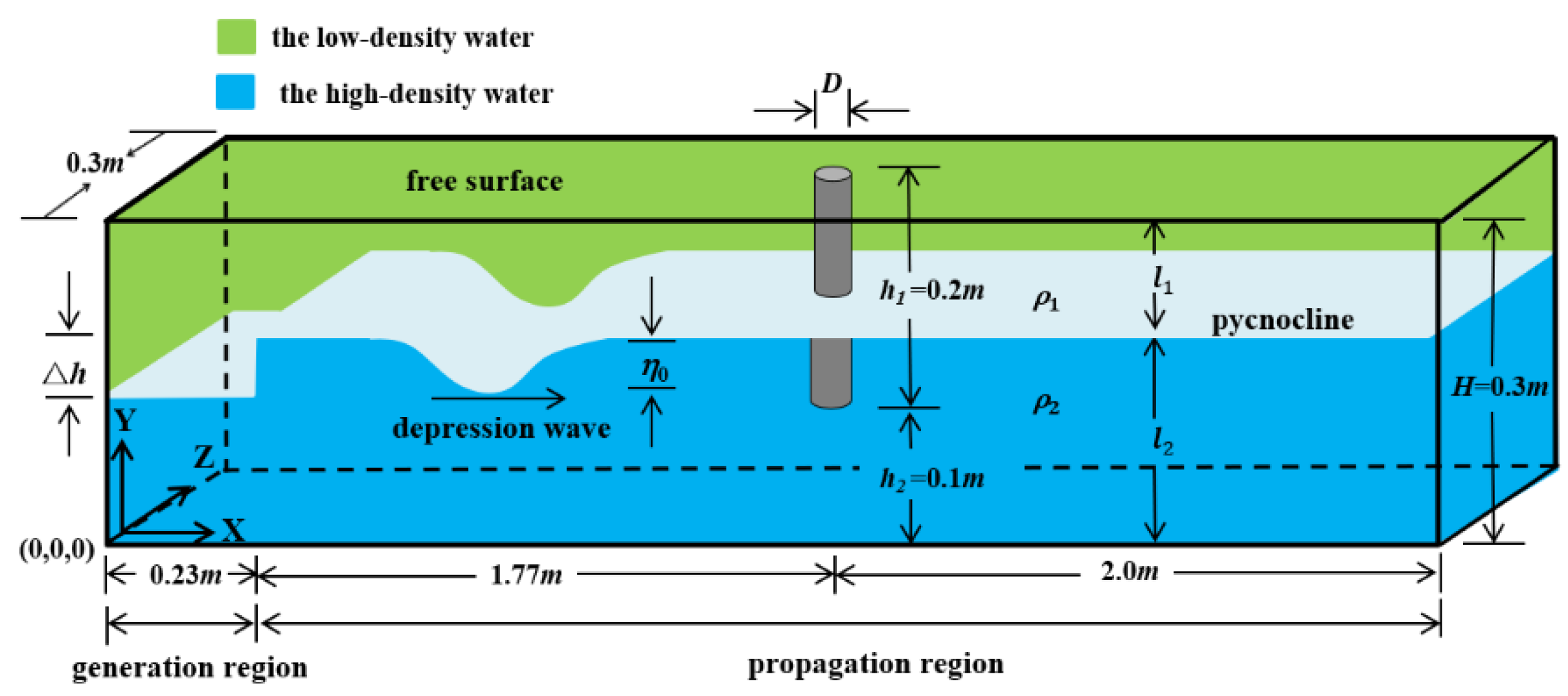
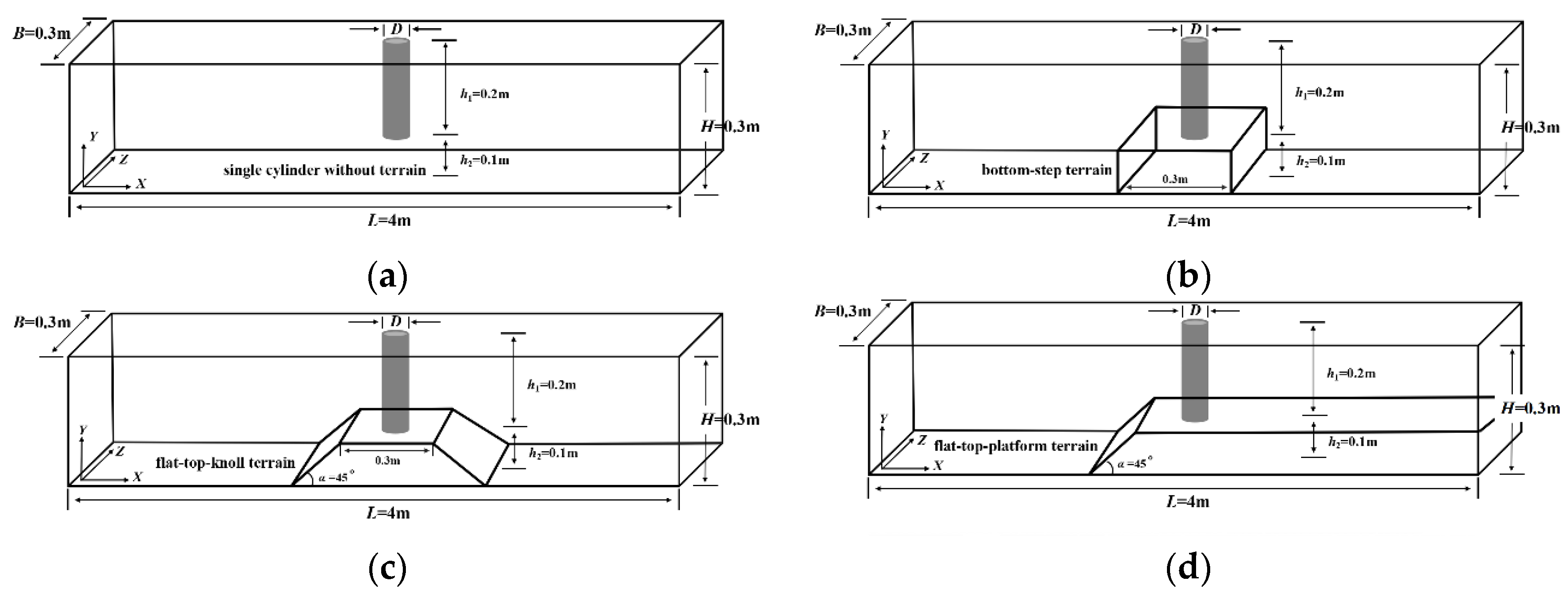
2.4. Establishment of a Numerical Tank

In the current study, the three-dimensional numerical terrain models are established based on a single-cylinder (SC, without terrain) tank model. The dimensions of this numerical model are 4.0 m long (X) × 0.3 m high (Y) × 0.3 m wide (Z), see Figure 1. A SC with a diameter D = 0.05 m and a length h₁ = 0.2 m is placed on the centerline in the spread direction (Z). The cylinder bottom center is located at (x, y, z) = (2.0, 0, 0.15) m. By using the gravity collapse approach to motivate the IWs [11], the numerical tank is separated into the IW generation region (x = 0–0.23 m) and the IW propagation region (x = 0.23–4 m), where Δh is the thickness difference in the pycnocline between the two regions, and η₀ is the initial amplitude.

In the stratified fluid environment, the upper layer is defined as the lower-density water layer with density ρ₁ = 0.998 g/cm³ and depth l₁ = 0.075 m, and the lower layer is defined as the higher-density water layer with density ρ₂ = 1.017 g/cm³ and depth l₂ = 0.225 m, respectively. Therefore, the total water depth of the tank H is kept at 0.3 m.

The generation and propagation of IWs of depression are simulated by the LES method [12]. The governing equations are discretized by the finite-volume method. The PISO algorithm is employed to ensure mass conservation and obtain the pressure field by coupling the velocity-pressure terms [13,14]. The second-order central differential scheme, the second-order upwind scheme, and the second-order implicit scheme are adopted to discretize the diffusion term, the convection term, and the time step, respectively.

Nonslip solid-rigid walls are chosen to define the numerical tank left wall (upstream boundary), the sidewalls, the bottom, and the cylinder periphery. A “Sommerfeld radiation” boundary condition is used to define the tank’s right wall (downstream boundary) [15] to avoid the reflection of IWs. The model top boundary is specified by the rigid-lid approximation [16] to neglect the surface waves. Surface waves are usually very small compared to the IWs [17], so the rigid-lid approximation is reasonable for the water surface.

2.5. Numerical Model Verification

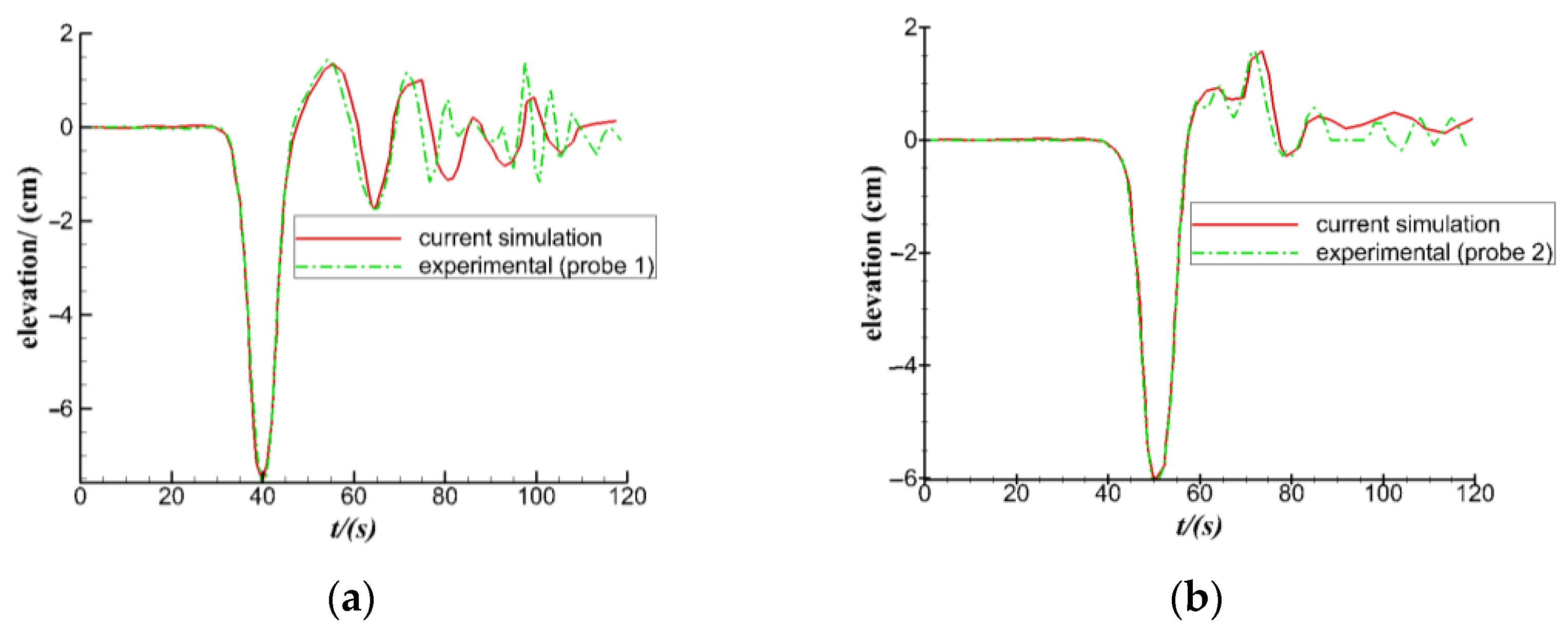
2.5.1. Verification by Physical Model Test

A physical model test conducted by Chen [18] is applied to verify the numerical model. The physical model tank with dimensions of length × width × depth = 12 m × 0.5 m × 0.7 m is illustrated in Figure 2. The thicknesses of the upper freshwater layer are 0.1 m with a density of 0.998 g/cm³, and the thicknesses of the lower saline layer are 0.4 m with density of 1.030 g/cm³. In the initial phase, there is a thickness difference controlled by a gate in the pycnocline between the IW generation region and the IW propagation region, which is similar to Figure 1 above. By lifting the gate, a leading IW of depression is motivated by the gravity collapse (caused by the thickness difference) method and propagates toward the tank’s left end [19], as shown in Figure 2. Two ultrasonic probes fixed in the tank top were adopted to capture the IWs spatial distribution in the propagation region of the numerical tank. A triangular bar was fixed between the probes, and the basis length Lw was equal to the wavelength.

The evolution of IWs excited by the current numerical simulation is compared with the physical model results of Chen [18] for verification. The comparison results of the verification, see Figure 3, presents that the simulation results agree well with the physical model results. Consequently, in this study, it is reasonable to adopt the numerical model for studying the IW interactions with cylinders and terrain.

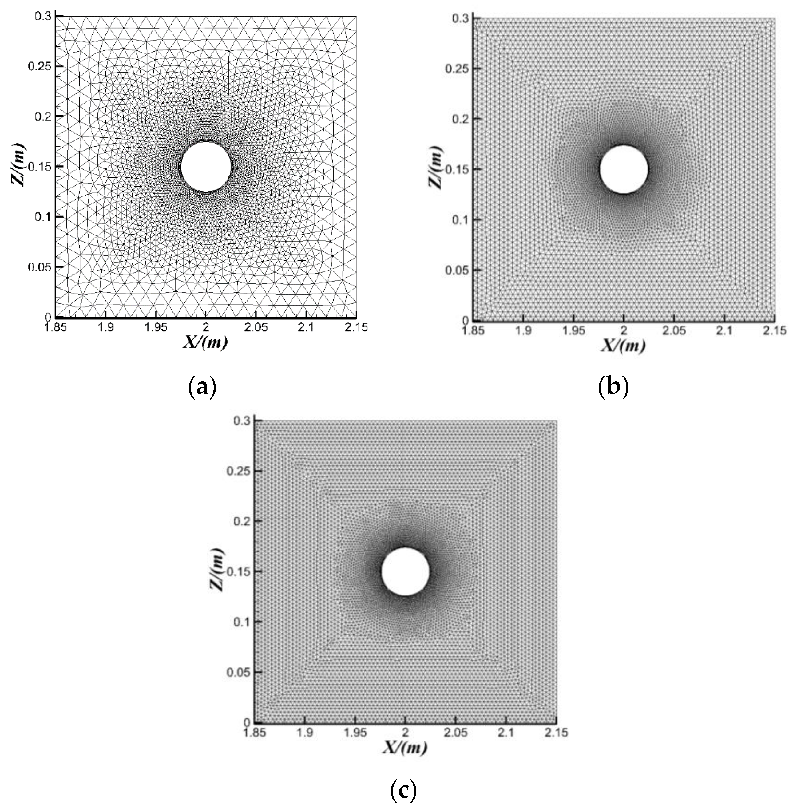
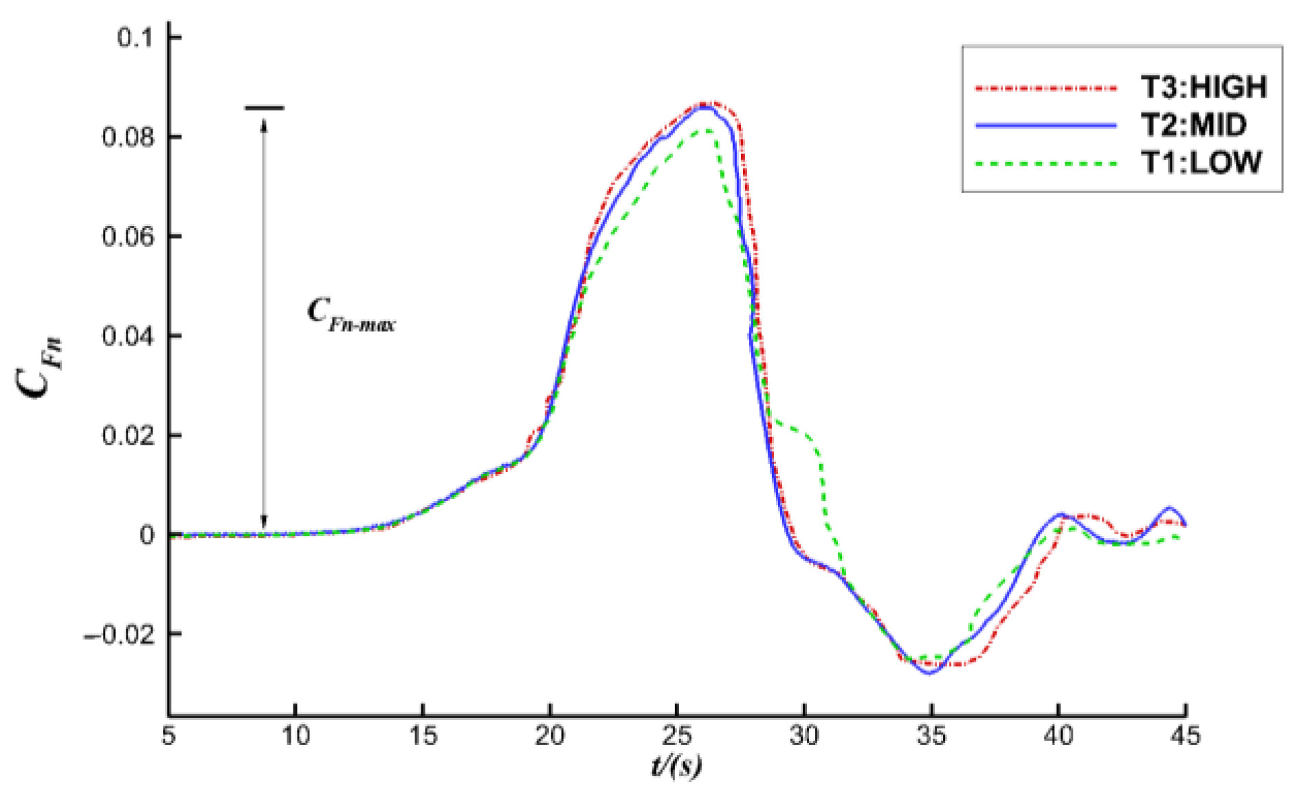
2.5.2. Grid Independence Test

The grid-size convergence analysis of the single cylinder (SC) without terrain is carried out in this section. Three cases of different grid types are set according to the differences in the number of nodes on the cylinder periphery, as illustrated in Figure 4. The details of the calculation cases are shown in

Table 1. The cases of grid-size independence test, ƞ₀/H = 0.0575.

No.	Case	∆t (s)	CFn-max	Elements Number
1	T1 (low density)	0.02	0.0810	525,454
2	T2 (moderate density)	0.01	0.0857	2,384,640
3	T3 (high density)	0.006	0.0862	3,318,278

.

In the current study, $C_{F_n}$ is used to define the dimensionless horizontal total force on the cylinder, which is calculated by the following formula:

$$C_{F_n}=\frac{F_n}{\rho gAH}$$

(8)

where, $F_n$ stands for the horizontal total force on the cylinder; g stands for the gravitational acceleration; A stands for the cylinder windward surface area (cylinder frontal side); and H is the total water depth of the tank.

The numerical results of the three different grid densities are illustrated in Figure 5. The force trend of the horizontal total force in the low-density grid is different from that in the medium-density grid, and the maximum horizontal force difference in the horizontal force in the two cases is about 0.5%. At the same time, the maximum horizontal force difference between medium-density grid and high-density grid is only approximately 0.05%, and C_Fn in T₂ almost coincides with that in T₃ over time. Therefore, the grid independence test results show the convergence of the grids. Consequently, the moderate gird density (case T₂) is sufficiently fine enough to discretize the computational domain, which can be adopted in the rest numerical simulations.

3. Result and Analysis

A nonuniform bottom is very common, such as bottom-step terrain [20], flat-top-knoll terrain [21], and flat-top-platform terrain [22]. To further explore the IW mechanical characteristics for the cylinder over terrain, one case of SC and three cases of different types of terrain are selected for comparative analysis, as shown in Figure 6a–d, including the SC model (Case N₁), the bottom-step terrain model (Case N₂), the flat-top-knoll terrain model (Case N₃), and the flat-top-platform model (Case N₄).

In this study, the stratified characteristic parameters (the water depth ratio l₁/l₂ of the two water layers, and the density difference Δρ between the two water layers) and the dimensionless IW amplitude η₀/H are consistent: the upper water depth l₁ = 0.075 m, the lower water depth l₂ = 0.225 m, making l₁/l₂ = 0.33; Δρ = 0.019 g/cm³, η₀/H = 0.0575. The diameter of the cylinder is 0.05 m, the length of the cylinder h₁ = 0.2 m, and the coordinates of the center of the cylinder bottom are (2, 0.1, 0.15) XYZ. The height difference between the cylinder bottom and the tank bottom is h₂ = 0.1 m. The lengths of the terrain platform in Cases N₂, N₃, and N₄ are 0.3 m, 0.3 m, and 2.15 m, respectively, and the slope angles α in Cases N₃ and N₄ are 45°. Schematic diagrams of numerical tank for the four cases are shown in Figure 6a–d, and the cases introduction is presented in

Table 2. Case introduction for different terrains.

No.	Case	h1/h2	η0/H	CFn-max
1	Single cylinder (N1)	0.33	0.0575	0.0857
2	Bottom-step terrain (N2)	0.33	0.0575	−0.0683
3	Flat-top-knoll terrain (N3)	0.33	0.0575	−0.0692
4	Flat-top-knoll terrain (N4)	0.33	0.0575	−0.0753

.

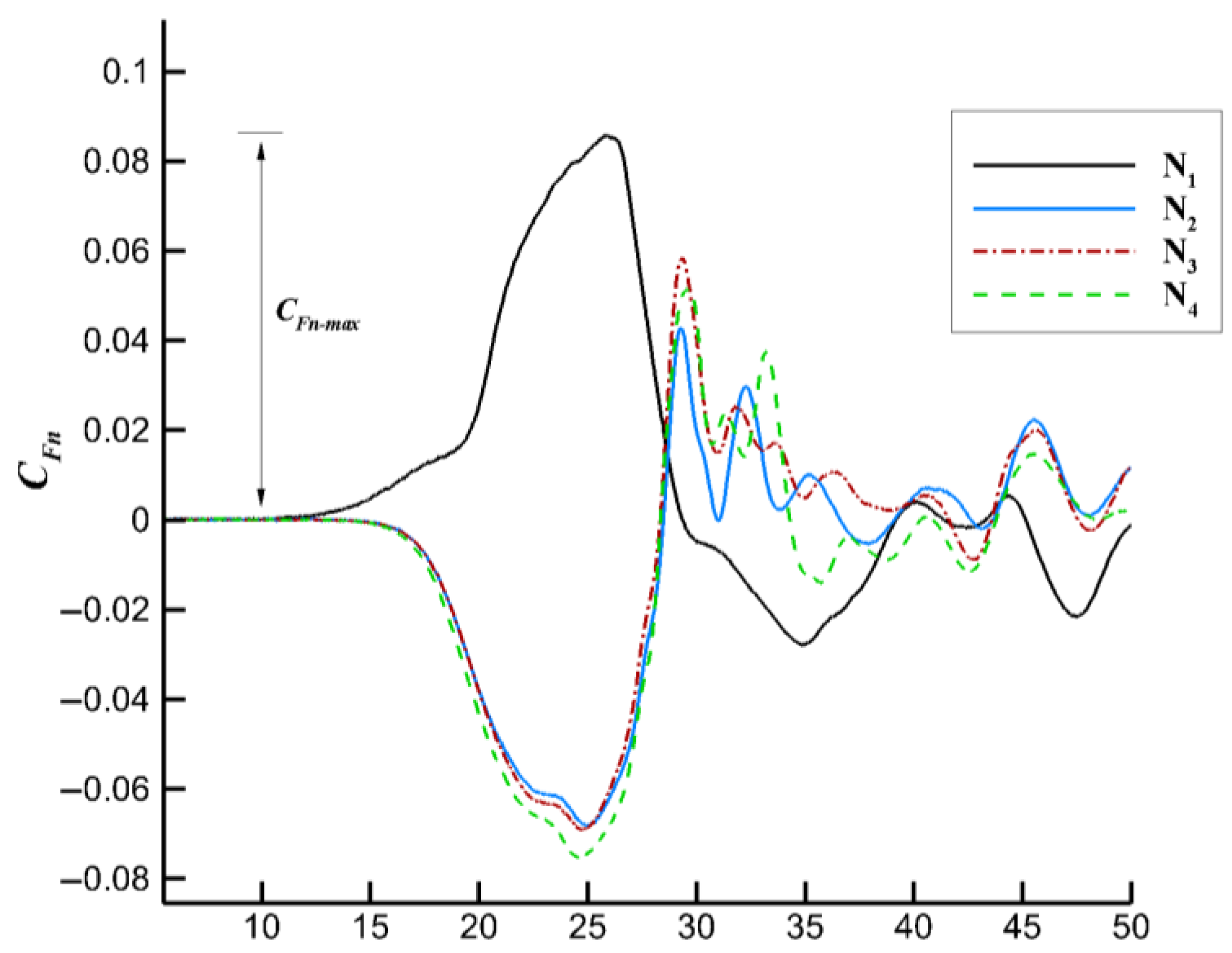
3.1. Coupled Influence of Terrain and IWs on the Forces on the Cylinder

Figure 7 shows the graphs of C_Fn on the cylinder vs. time t for the SC case and the three terrain cases. The figure presents that the peak value of C_Fn in the cylinder of the N₁ case is significantly larger than that of the other three terrain cases, indicating that the bottom topography significantly changes the IW forces on the cylinder and makes the IW forces peak value C_Fn-max change from positive to negative. Obvious negative peaks of C_Fn appear in the three terrain cases N₂, N₃, and N₄ when the IWs are close to the front edge of the terrain. The reduction in the lower layer depth of IW due to the topographical factors causes a shallow-water effect, and the strength of the fluid flow field in the lower layer around the bottom terrain is enhanced. Moreover, the negative forces applied to the cylinder over the terrain result in the negative peak value of C_Fn. As shown in Figure 8, the negative forces on the cylinder in the lower layer in cases N₂, N₃, and N₄ are much greater than those in case N₁, which can also explain the difference in the peak value between N₁ and N₂–N₄ in Figure 7. As a result, the shallow-water effect enhances the strength of the flow field around the cylinder in the lower layer, thereby causing a greater negative force on the lower parts of the cylinder.

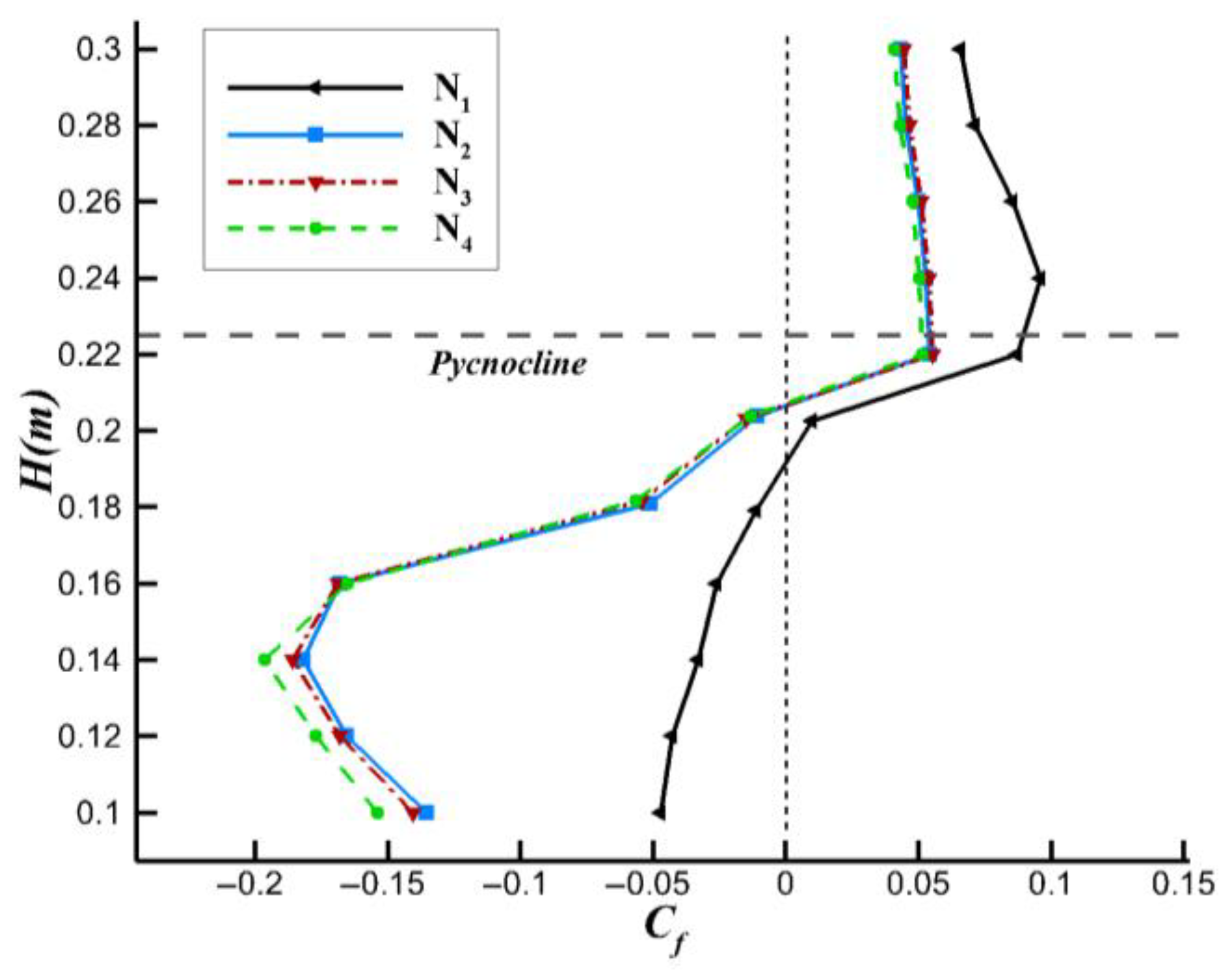
3.2. Comparison of the Vertical Distribution of the Force on the Cylinder in Different Cases

The calculation results corresponding to the time C_Fn = C_Fn-max of all the cases (as shown in Figure 8, t ≈ 25 s, the time of the most unfavorable forces on the cylinder) are selected for analysis. By further analyzing the stress mechanism of the cylinder over different terrains, the cylinder body is divided into ten parts along the vertical direction, and a section is taken at a separation of 0.02 m. The parts in the upper layer are defined as “upper parts”, and the parts in the lower layer are called “lower parts”. The pycnocline between the upper parts and lower parts is at the depth of 0.225 m. The vertical distribution of the non-dimensional horizontal forces C_f at various water depths in all the cases are shown in Figure 8. The calculation expression of C_f is similar to Equation (8) for C_Fn. C_f on the upper parts of the cylinder is positive, and the value in case N₁ condition is significantly greater than that in the other three cases. C_f on the lower parts of the cylinder becomes negative and the values in cases N₂, N₃, and N₄ are much greater than that in case N₁.

The pressure coefficient of the cylinder periphery at a certain depth section is $C_{Py}$, and the expression can be defined as follows:

$$C_{Py}=\frac{ 2\times (P_y-P_{oy})}{{\rho }_y{U}_{\max y}^2}$$

(9)

where P and U_max are the point pressure on the cylinder periphery and the maximum velocity, respectively; P_o is the point hydrostatic pressure on the cylinder periphery; and ρ is the fluid density. The subscript y denotes a certain depth y. In this paper, the values of y are 0.26 m and 0.14 m, which are the center heights of the upper and lower layers, respectively. The schematic diagram for the definition of the circumferential angle is illustrated in Figure 9, where the angel degrees ranging from 90° to 270° form the cylinder windward surface area (frontal side), and the angel degrees ranging from 270° to 90° from the lee side.

Figure 10a,b shows the distribution of the pressure coefficient C_p on the cylinder at Plane_y=0.26 (P_0.26 for short, y = 0.26 m) and Plane_y=0.14 (P_0.14 for short, y = 0.14 m) sections.

As shown in the Figure 10a of the pressure distributions in the upper layer (y = 0.26 m), the maximum pressure points on the periphery are all at the former stagnation points, and the lee sides of the cylinders are all immersed in the low-pressure areas. The pressure on the frontal sides is greater than that on the lee side, so the forces on the upper parts of the cylinder are generally positive. Moreover, the pressure on the frontal sides in case N₁ is significantly greater than that in cases N₂–N₄, resulting in the forces on the upper parts in case N₁ being significantly greater than those in cases N₂–N₄.

As shown in Figure 10b, the pressure distributions in the lower layer (y = 0.14 m), the high-pressure areas all appear near the cylinder lee sides. The pressure on the cylinder frontal sides is less than that on the lee sides, resulting in negative horizontal resultant forces on the lower parts (see Figure 8). Moreover, the differences in pressure between the frontal sides and the lee sides in cases N₂–N₄ are much greater than those in case N₁. Therefore, the reverse horizontal forces on the cylinder in cases N₂–N₄ are much greater than those in case N₁.

Combined with the vorticity contours, the pressure distribution characteristics of the cylinders are further analyzed below. The propagation direction of the IWs is defined as the positive direction. When the IWs pass through the cylinder, the flow direction in the upper water is the same as the wave direction, so that the frontal side of the upper parts is impacted by the IWs, while the vortexes are formed near the lee sides (as shown in Figure 11). Therefore, the pressure on the frontal side increases, while the pressure on the lee side immersed in the vortexes decreases. The pressure difference between the frontal side and lee side leads to a positive horizontal total force on the upper parts, and the maximum pressure point is at the former stagnation point. Moreover, Figure 11 shows that the vortices around the cylinder in the SC case are obviously different from those in the other three terrain cases, indicating that the existence of terrain weakens the horizontal forces on the upper parts to a certain extent.

In the lower layer, the wave propagation direction is opposite to the flow propagation direction, and the vortices of the low-pressure region are formed near the frontal side of the cylinder (see Figure 12), thus reducing the pressure on the frontal side. The pressure difference between the frontal side and lee side results in the reverse horizontal resultant force, as shown in Figure 12. In addition, combined with Figure 13, the shallow-water effect occurs when IWs propagate to the bottom terrain [23,24], which strengthens the flow field near the terrain in the lower layer and makes the lower parts subject to the impact of the additional reverse wave fluid. Additionally, although in the four cases the vortices all appear near the frontal sides of the lower parts, the vortices in the SC case are significantly different from those in the other three terrain cases due to the influence of the topographic factors, resulting in the difference between the horizontal resultant forces on the lower parts in the terrain cases and the no terrain case.

In summary, the existence of bottom terrains weakens the forces on the upper parts of the cylinder in the upper layer fluid, and due to the shallow-water effect in the lower layer, the lower parts of the cylinder are subject to greater horizontal resultant forces in the reverse wave direction.

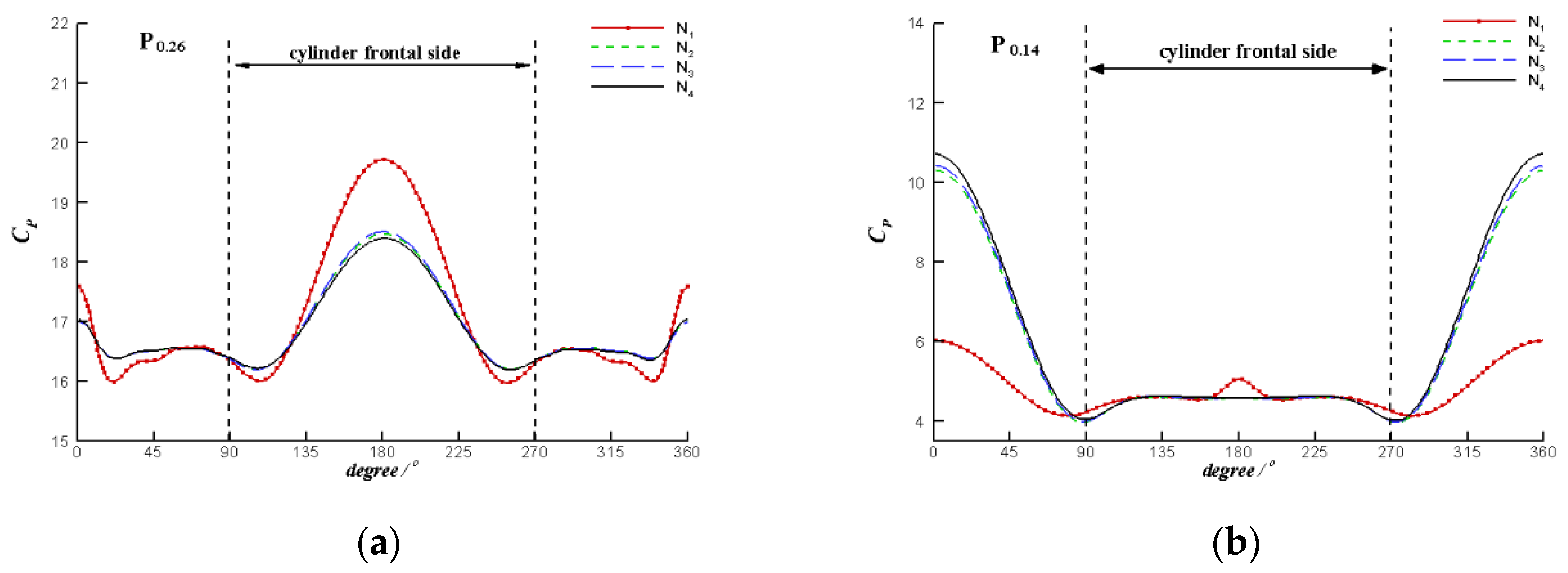
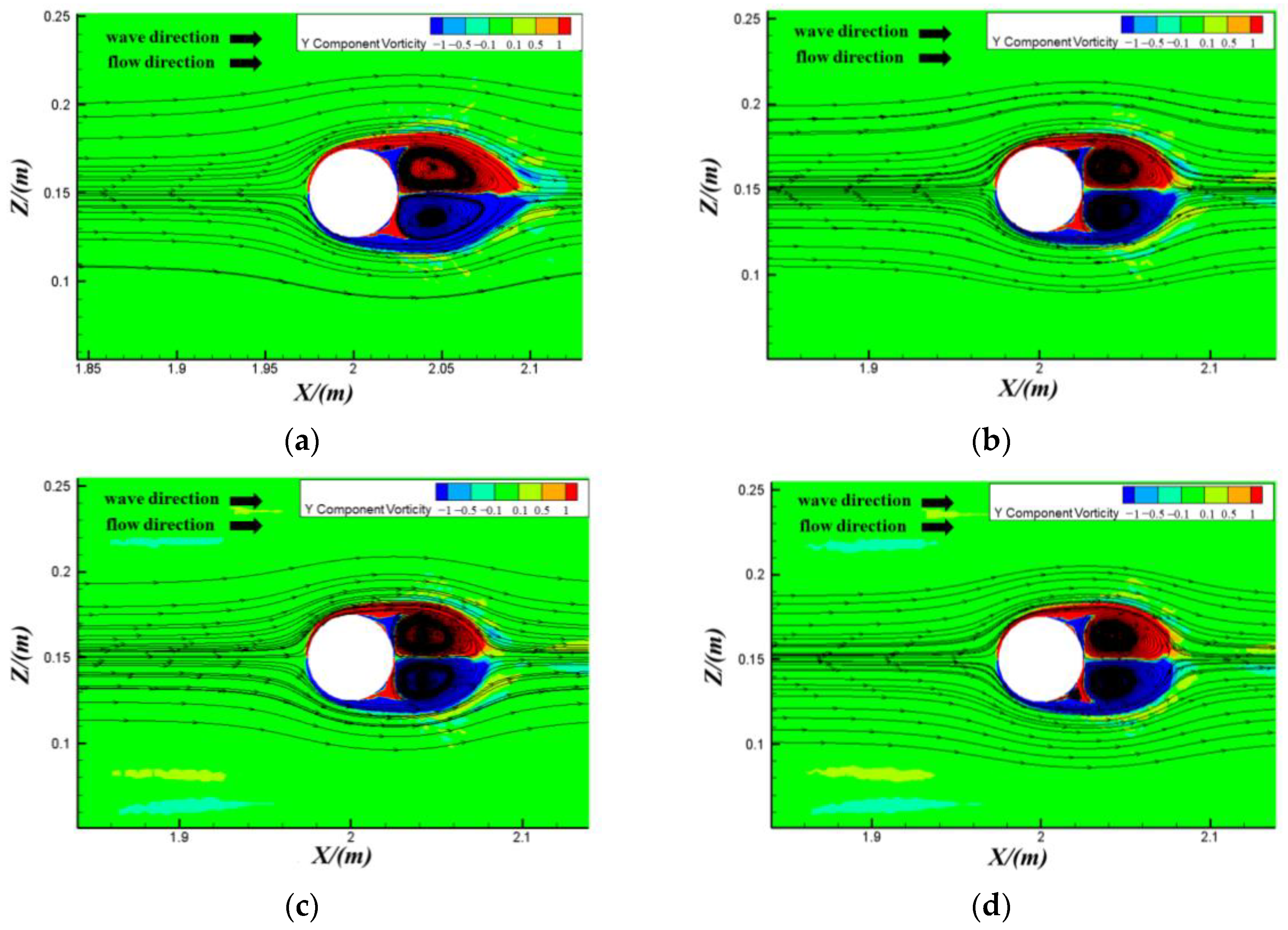
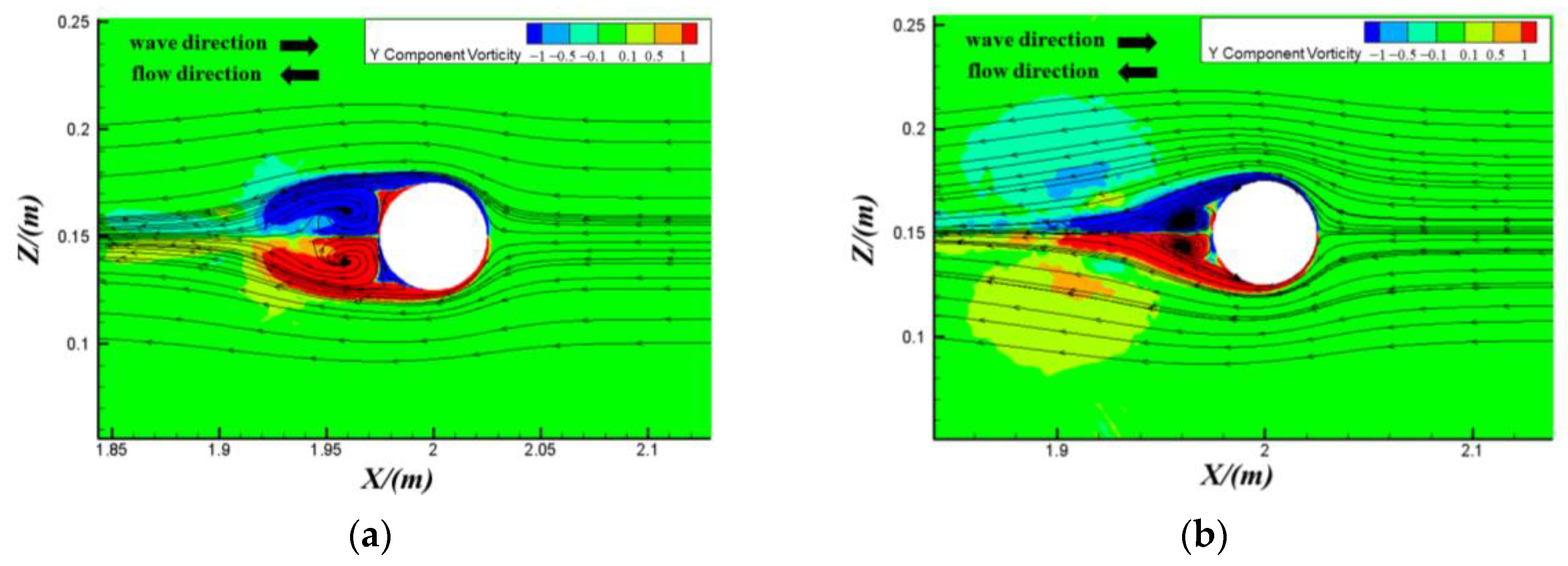
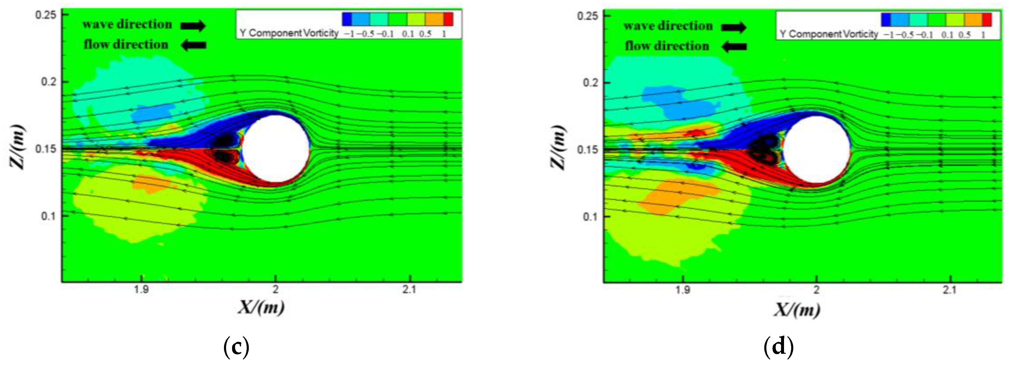
3.3. Variation in the Flow Field around the Cylinder under Different Cases

By comparing the flow field distributions of the SC case (N₁) with the terrain cases (N₂–N₄) in Figure 13a–d, it is found that, when the IWs reach the bottom terrain, vortexes can be found near the frontal side of the terrain, but no obvious vortex appears in case N₁. The vortexes are generated by the coupled effects of the IWs, the topography, and the shallow-water effect. Compared with the SC case, when the IWs propagate over the terrain, the interactions between the IWs and the terrain make the flow field around the cylinder more complex and changeable, especially near the lower parts of the cylinder. As a result, the complex hydrodynamic environment caused by the IWs and the terrains compels the cylinder to experience larger forces.

3.4. Influence of the Amplitudes on the IWs Forces and the Flow Field over the Terrain

On the base of the above research, the terrain is a key consideration to explore the hydrodynamic characteristics in IW environment, but the IWs amplitudes also have a big effect on the forces on and the flow field around the cylinder [25,26]. Therefore, more calculation results of the influence of the amplitudes on IWs forces are presented to study the research further in the following. The cases introduction is presented in

Table 3. Case introduction for different amplitudes.

No.	Case	h1/h2	η0/H	CFn-max	RFn-max
1	S1	0.33	0.0275	0.0245	17.6%
2	F1	0.33	0.0275	0.0202
3	S2	0.33	0.0384	0.0428	17.5%
4	F2	0.33	0.0384	−0.0353
5	S3	0.33	0.0494	0.0664	13.9%
6	F3	0.33	0.0494	−0.0572
7	S4	0.33	0.0575	0.0857	12.1%
8	F4	0.33	0.0575	−0.0753
9	S5	0.33	0.0674	0.132	34.5%
10	F5	0.33	0.0674	−0.0864

. The case S stands for the SC case and the case F stands for the flat-top-platform terrain case, where the subscripts 1-5 indicate the different amplitudes ranging from 0.0275 to 0.0674.

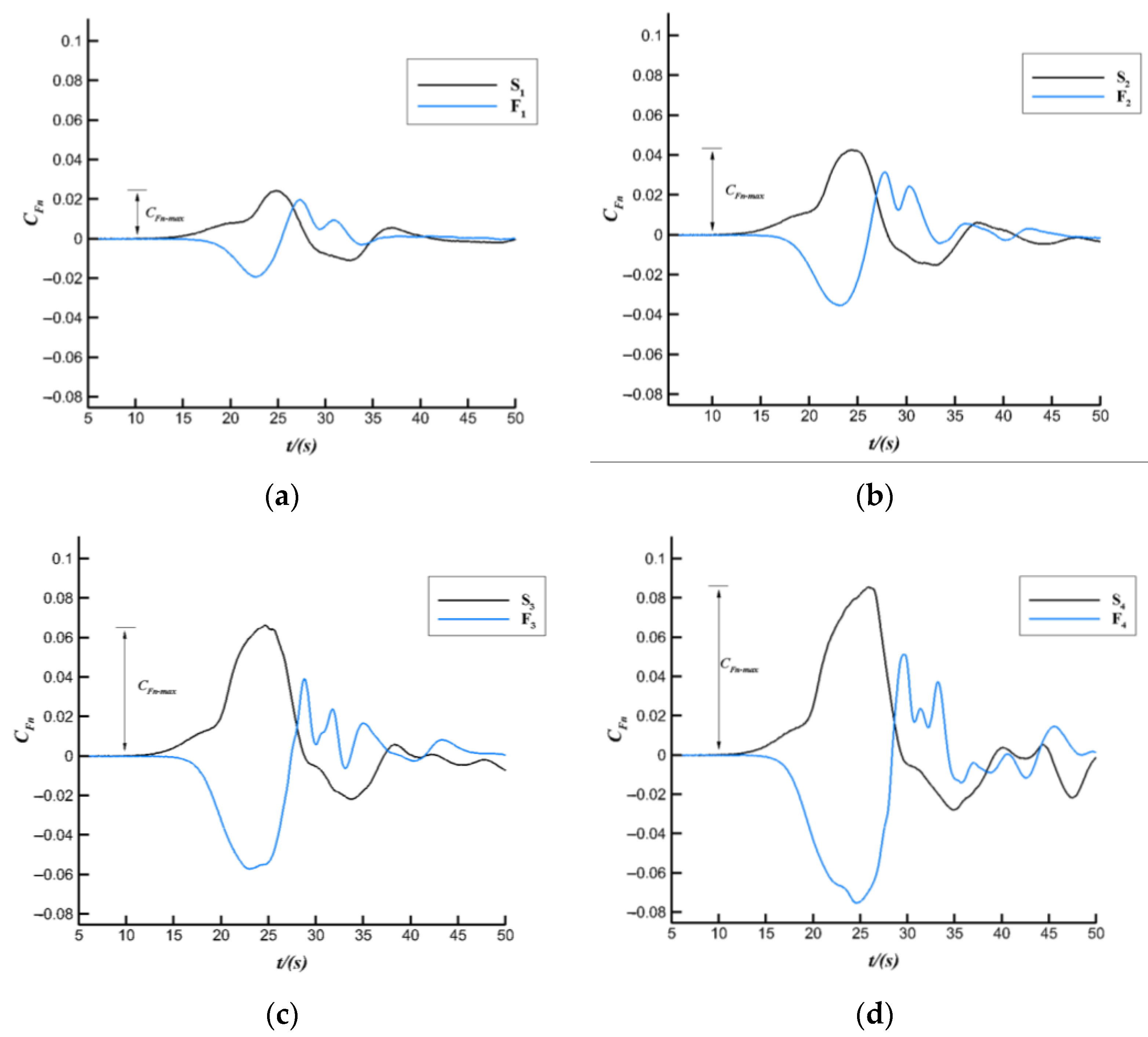
3.4.1. Influence on the IWs Forces

The comparison of C_Fn vs. time t between the case S (SC) and the case F (flat-top-platform terrain) under different amplitudes conditions are shown in Figure 14. On the whole, with the increase of the IW amplitude, the forces on the single cylinder increase, and the duration curve of the IW forces on cylinder are all similar in all the cases. Under the small amplitude condition of η₀/H = 0.0275 (see Figure 14a), the IW forces peaks C_Fn-max for the case S₁ and the case F₁ are both positive. C_Fn-max for the cases F₂–F₅ turn negative as the amplitude increases, while C_Fn-max for the cases S₂–S₅ still keep positive (see Figure 14b–e). Meanwhile, a percentage parameter R_Fn-max is applied here to specify the differences of C_Fn-max between the cases S and the cases F, and the expression can be defined as follow:

$$R_{Fn-max}=\frac{{{(C}_{Fn-max})}_S-\left|{{(C}_{Fn-max})}_F\right|}{{{(C}_{Fn-max})}_S}$$

(10)

where ${{(C}_{Fn-max})}_S$ and ${{(C}_{Fn-max})}_F$ are the IW forces peaks on the cylinder for the case S and the case F, respectively.

As can be seen from the Table 3, R_Fn-max decreases as the IW amplitudes η₀/H increase from 0.0275 to 0.0575 but it sharply increases to 34.5% when η₀/H reaches 0.0674. This can be explained by the flow field and density distribution characteristics as illustrated in Figure 15e and Figure 16e. When IW with large amplitude propagates to the bottom terrain, the interaction between the IW and the terrain is intensified and the shallow-water effect occurs, which strengthens the flow field strength near the terrain in the lower layer and influences the force on the cylinder. A phenomenon of “elevation” simultaneously occurs because of the “blockage” effect caused by the bottom topography, which directly reflects the influence of the existing terrain on the flow field near the cylinder.

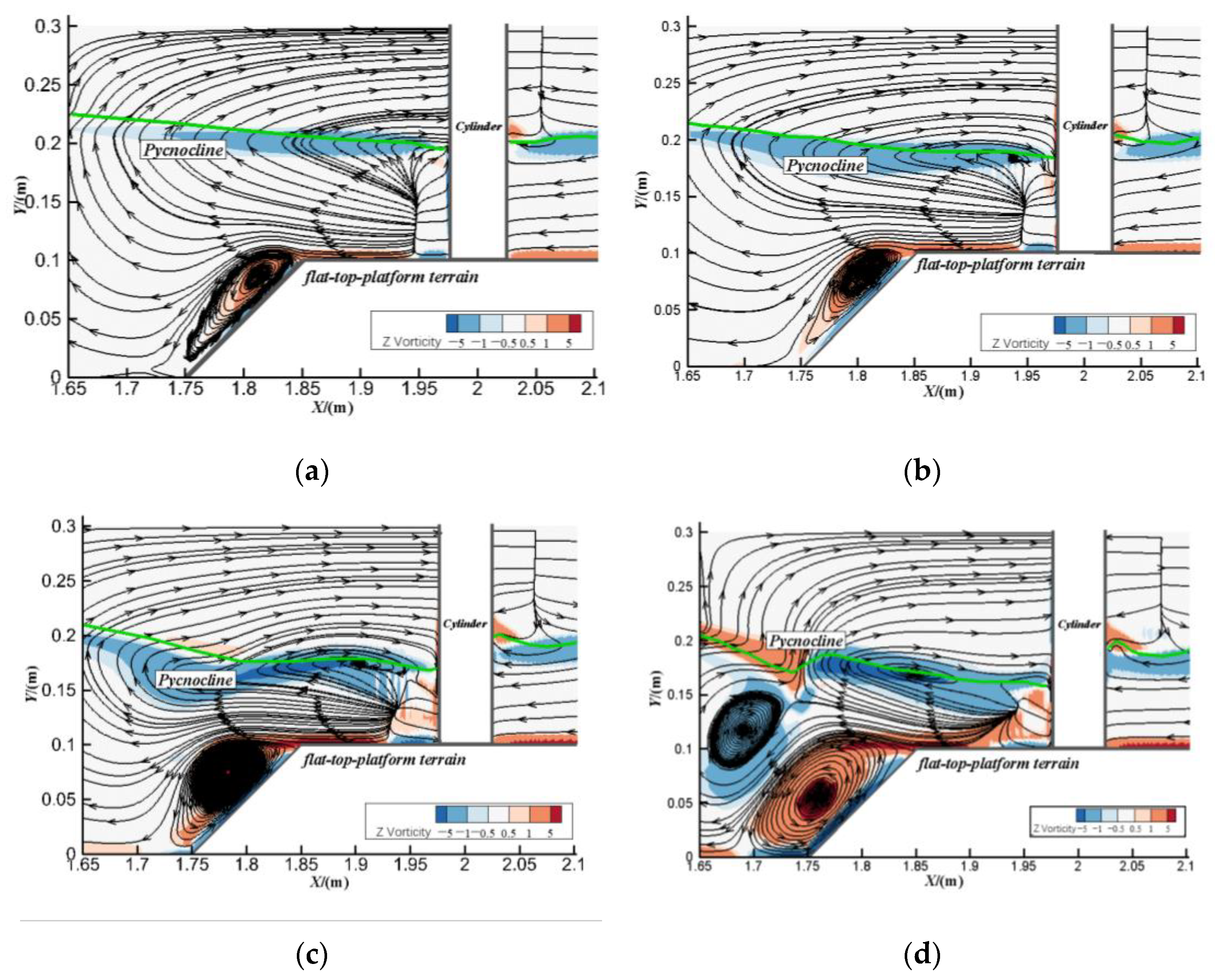
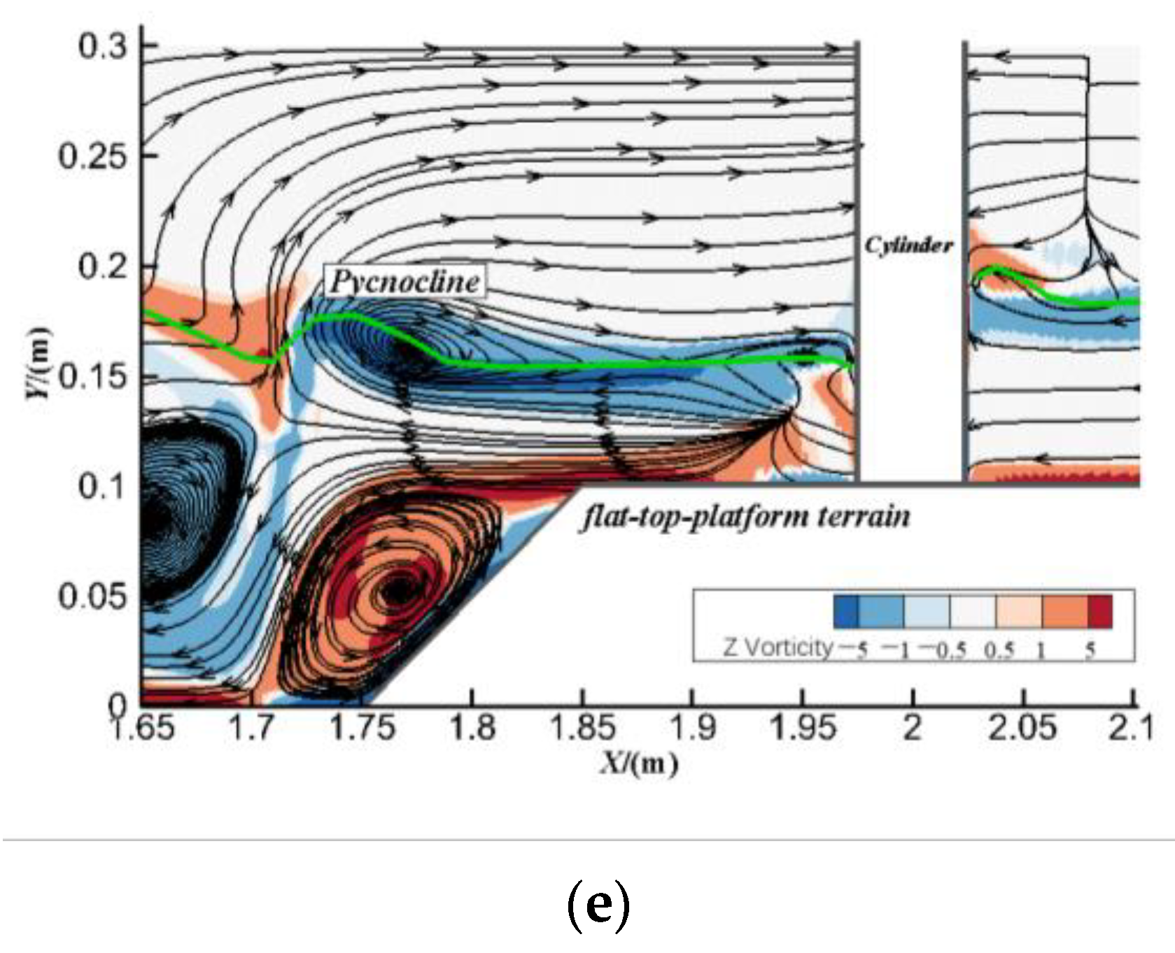
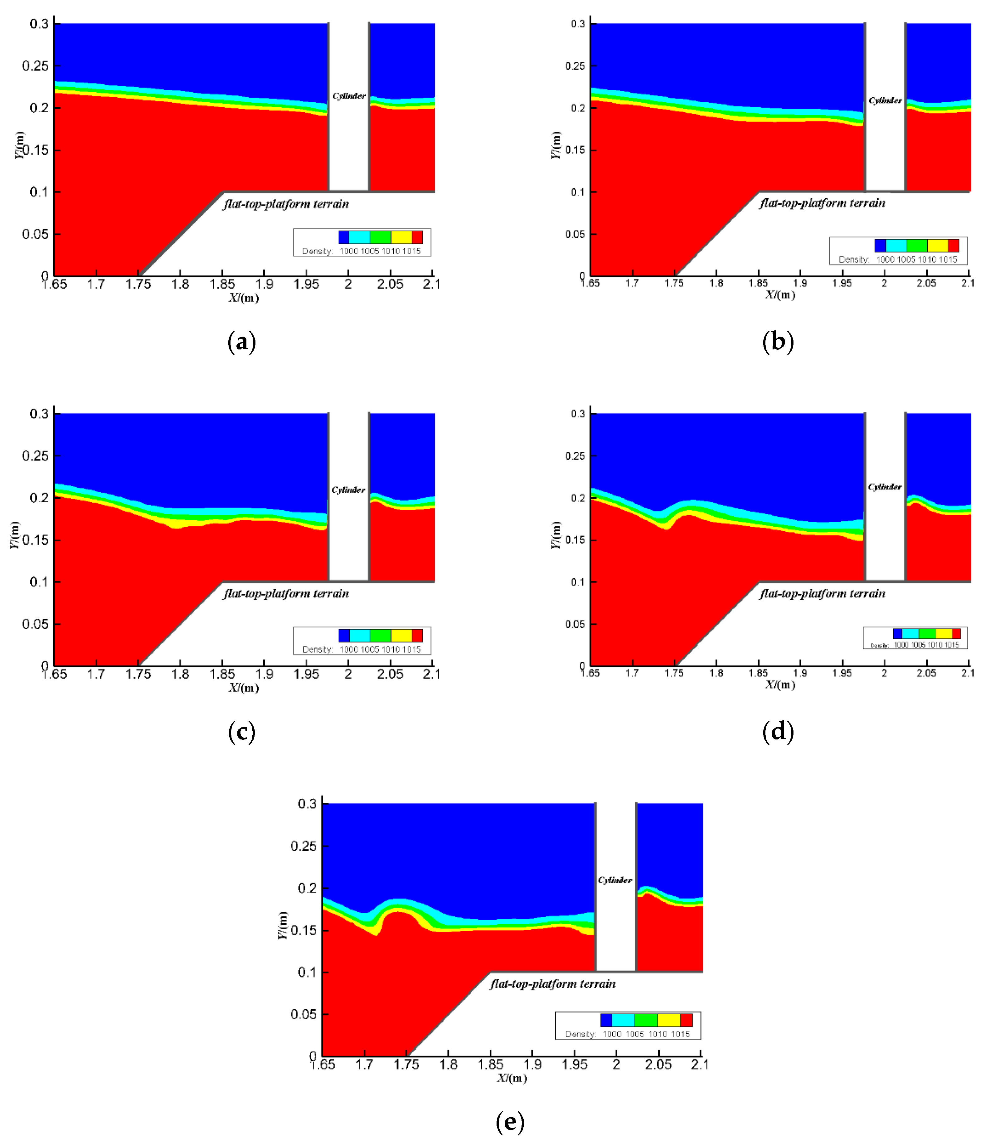
3.4.2. Influence on the Flow Field

The flow field distribution characteristics of different amplitudes conditions are plotted in Figure 15a–e. With the increase of the wave amplitude, the interaction between the IW and the terrain as well as the flow field intensity are both enhanced. The vortices can be found on the bank slope in all the cases, but the size of the vortex is obviously different when the amplitude changes. It is obvious that the vortex size increases with the amplitude, and more than one vortex appears when the amplitude exceeds 0.0575, which can be found in Figure 15d,e.

The density distribution characteristics plotted in Figure 16a–e also give evidence to present the interaction between the IWs and the terrain. With the increase of IW amplitude, the IW pattern is more strongly disturbed by the terrain. IW propagating over the bank slope is partially reflected, causing a remarkable “blockage” near the terrain and a “elevation” phenomenon in the reverse wave propagation direction as illustrated in Figure 16e. Therefore, the increase of the interaction strength between the IWs and the terrain could not only cause greater horizontal forces on the lower parts of the cylinder, but also make the flow field around the terrain more complex, further affecting the mechanical characteristics of the cylinder.

4. Conclusions

A 3D numerical tank model of a flume with internal waves and terrain is set up to research the mechanics characteristics of the cylinder in an IW-terrain coupled environment. The main described are as follows:

(1)

The topographic factors of the terrain significantly affect the IW forces on the cylinder. There is a strong distinction between the SC case and the three terrain cases: in the SC case, the maximum resultant forces on the cylinder are positive, and the maximum resultant forces are negative in the terrain cases.

(2)

Compared with the SC case, the shallow-water effect caused by the IW-terrain coupled environment enhances the strength of the flow field around the cylinder, so that the lower parts of the cylinder are subjected to larger forces in the reverse wave direction.

(3)

Compared with the SC case, when the IWs propagate over the terrain, the interactions between the IWs and the terrain make the flow field around the cylinder more complex and changeable. As a result, the complex hydrodynamic environment compels the cylinder to experience larger forces.

(4)

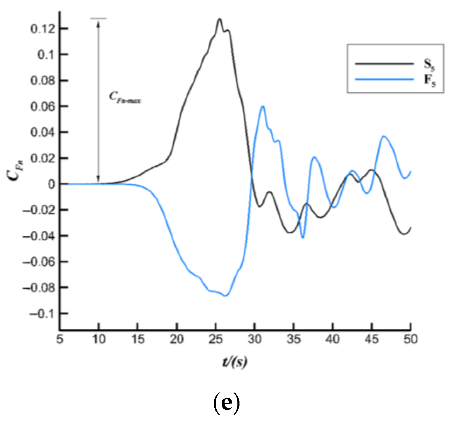
A percentage parameter R_Fn-max is applied in this research to specify the differences of C_Fn-max between the SC case and the terrain case. R_Fn-max decreases as the IW amplitude increases when the amplitude is relatively small, but it sharply increases when amplitude is large enough. It is can be explained by the shallow-water effect. When IWs with large amplitude propagate to the bottom terrain, the interaction between the IW and the terrain is intensified and the shallow-water effect occurs, which strengthens the flow field strength near the terrain in the lower layer.

(5)

With the increase of IW amplitude, the interaction between the IW and the terrain is enhanced. Vortices can be found on the bank slope in all the cases, but the size of the vortices is obviously different when amplitude changes. The vortex size increases with the amplitude, and more than one vortex appears when the amplitude is large enough.

(6)

With the increase of the IW amplitude, the IW pattern is more strongly disturbed by the terrain. IW propagating over the bank slope is partially reflected, causing a “blockage” near the terrain and a “elevation” in the reverse wave propagation direction. Therefore, the intensification of the interaction strength between the IWs and the terrain could not only cause greater horizontal forces on the lower parts of the cylinder, but also make the flow field around the terrain more complex.

References

1. Mei, Y.; Wang, J.; Huang, S.; Mu, H.; Chen, X. Experimental investigation on the optical remote sensing images of internal solitary waves with a smooth surface. Acta Oceanol. Sin. 2019, 38, 124–131. [Google Scholar] [CrossRef]
2. Wang, X.; Zhou, J.-F.; Wang, Z.; You, Y.-X. A numerical and experimental study of internal solitary wave loads on semi-submersible platforms. Ocean Eng. 2018, 150, 298–308. [Google Scholar] [CrossRef]
3. Xu, W.; Lin, Z.Y.; You, Y.X.; Yu, R. Numerical Simulations for the Load Characteristics of Internal Solitary Waves on a Vertical Cylinder. J. Ship 2017, 21, 1071–1085. [Google Scholar]
4. Colosi, J.A.; Kumar, N.; Suanda, S.H.; Freismuth, T.M.; MacMahan, J.H. Statistics of Internal Tide Bores and Internal Solitary Waves Observed on the Inner Continental Shelf off Point Sal, California. J. Phys. Oceanogr. 2018, 48, 123–143. [Google Scholar] [CrossRef]
5. Moum, J.N.; Farmer, D.M.; Smyth, W.D.; Armi, L.; Vagle, S. Structure and Generation of Turbulence at Interfaces Strained by Internal Solitary Waves Propagating Shoreward over the Continental Shelf. J. Phys. Oceanogr. 2003, 33, 2093–2112. [Google Scholar] [CrossRef]
6. Timothy, W. Internal Solitons on the Pycnocline: Generation, Propagation, and Shoaling and Breaking over a Slope. J. Fluid Mech. 1985, 159, 19–53. [Google Scholar]
7. Chen, M.; Chen, K.; You, Y.X. Experimental investigation of internal solitary wave forces on a semi-submersible. Ocean Eng. 2017, 141, 205–214. [Google Scholar] [CrossRef]
8. Jia, T.; Liang, J.J.; Li, X.-M.; Sha, J. SAR Observation and Numerical Simulation of Internal Solitary Wave Refraction and Reconnection Behind the Dongsha Atoll. J. Geophys. Res. Oceans 2018, 123, 74–89. [Google Scholar] [CrossRef]
9. Chen, L.; Zheng, Q.; Xiong, X.; Yuan, Y.; Xie, H.; Guo, Y.; Yu, L.; Yun, S. Dynamic and Statistical Features of Internal Solitary Waves on the Continental Slope in the Northern South China Sea Derived From Mooring Observations. J. Geophys. Res. Oceans 2019, 124, 4078–4097. [Google Scholar] [CrossRef]
10. Germano, M.; Piomelli, U.; Moin, P.; Cabot, W.H. A dynamic subgrid-scale eddy viscosity model. Phys. Fluids 1991, 3, 1760–1765. [Google Scholar] [CrossRef]
11. Michallet, H.; Barthelemy, E. Experimental study of large interfacial solitary waves. Fluid Mech. 1998, 366, 159–177. [Google Scholar] [CrossRef]
12. Camassa, R.; Choi, W.; Michallet, H.; Rusås, P.-O.; Sveen, J.K. On the realm of validity of strongly nonlinear asymptotic approximations for internal waves. J. Fluid Mech. 2006, 549, 1–23. [Google Scholar] [CrossRef]
13. Li, X.; Ren, B.; Wang, G.Y.; Wang, Y.X. Numerical simulation of hydrodynamic characteristics on an arx crown wall using volumn of fluid method based on BFC. J. Hydrodyn. 2001, 23, 767–776. [Google Scholar] [CrossRef]
14. Chen, Y.X. Flow simulation of car air conditioner duct based on simple algorithm. Mech. Eng. 2008, 11, 111–112. [Google Scholar]
15. Cao, Y.; Ye, Y.T.; Liang, L.L.; Zhao, H.; Jiang, Y.; Wang, H.; Wang, J. Uncertainty analysis of two-dimensional hydrodynamic model parameters and boundary conditions. J. Hydroelectr. Eng. 2018, 37, 47–61. (In Chinese) [Google Scholar]
16. Forgia, G.L.; Sciortino, G. Free-surface effects induced by internal solitons forced by shearing currents. Phys. Fluids 2021, 33, 072102. [Google Scholar] [CrossRef]
17. Zhu, H.; Wang, L.L.; Avital, E.J.; Tang, H.W.; Williams, J.J.R. Numerical Simulation of Shoaling Broad-Crested Internal Solitary Waves. J. Hydraul. Eng. 2017, 143, 04017006. [Google Scholar] [CrossRef]
18. Chen, C.-Y. Amplitude decay and energy dissipation due to the interaction of internal solitary waves with a triangular obstacle in a two-layer fluid system: The blockage parameter. J. Mar. Sci. Technol. 2009, 14, 499–512. [Google Scholar] [CrossRef]
19. Chen, C.Y.; Hsu, J.R.C.; Chen, C.W.; Chen, H.H.; Kuo, C.F. Generation of internal solitary wave by gravity collapse. J. Mar. Sci. Technol. 2007, 15, 1–7. [Google Scholar] [CrossRef]
20. Talipova, T.; Terletska, K.; Maderich, V.; Brovchenko, I.; Jung, K.T.; Pelinovsky, E.; Grimshaw, R. Internal solitary wave transformation over a bottom step: Loss of energy. Phys. Fluids 2013, 25, 032110. [Google Scholar] [CrossRef]
21. Cheng, C.Y.; Hsu, J.R.C.; Chen, M.H. An investigation on internal solitary waves in a two-layer fluid:Propagation and reflection from steep slopes. Ocean. Eng. 2007, 34, 171–184. [Google Scholar] [CrossRef]
22. Cheng, M.-H.; Hsu, J.R.-C.; Chen, C.-Y. Laboratory experiments on waveform inversion of an internal solitary wave over a slope-shelf. Environ. Fluid Mech. 2011, 11, 353–384. [Google Scholar] [CrossRef]
23. Shroyer, E.L.; Moum, J.N.; Nash, J. Observations of Polarity Reversal in Shoaling Nonlinear Internal Waves. J. Phys. Oceanogr. 2009, 39, 691–701. [Google Scholar] [CrossRef]
24. Sutherland, B.R.; Barrett, K.J.; Ivey, G.N. Shoaling internal solitary waves. J. Geophys. Res. Ocean. 2013, 118, 4111–4124. [Google Scholar] [CrossRef]
25. Wei, G.; Du, H.; Xu, X.; Zhang, Y.; Qu, Z.; Hu, T.; You, Y. Experimental investigation of the generation of large-amplitude internal solitary wave and its interaction with a submerged slender body. Sci. China Phys. Mech. Astron. 2014, 57, 301–310. [Google Scholar] [CrossRef]
26. Zou, P.; Bricker, J.D.; Uijttewaal, W. The impacts of internal solitary waves on a submerged floating tunnel. Ocean Eng. 2021, 238, 109762. [Google Scholar] [CrossRef]
Figure 1. Sketch map of the single cylinder (SC) numerical model.
Water 15 01598 g001
Figure 2. Schematic diagram of the physical model test [18].
Water 15 01598 g002
Figure 3. Validation results: (a) probe 1, (b) probe 2.
Water 15 01598 g003
Figure 4. Detail view of the unstructured mesh around a cylinder periphery: (a) T1, (b) T2, (c) T3.
Water 15 01598 g004
Figure 5. Numerical model verification results of the IWs forces on a cylinder of different mesh densities, ƞ0/H = 0.0575.
Water 15 01598 g005
Figure 6. Sketch map of numerical tank for four cases: (a) N1, (b) N2, (c) N3, (d) N4.
Water 15 01598 g006
Figure 7. Graphs of CFn on the cylinder vs. time t for various cases.
Water 15 01598 g007
Figure 8. Comparison diagram of layered horizontal resultant force under four working conditions, CFn = CFn-max.
Water 15 01598 g008
Figure 9. Schematic diagram for the definition of circumferential angle.
Water 15 01598 g009
Figure 10. Comparison of the pressure distribution between N1 and N2–N4. (a) y = 0.26 m, (b) y = 0.14 m.
Water 15 01598 g010
Figure 11. Plots of vorticity around the cylinder at P0.26: (a) N1, (b) N2, (c) N3, (d) N4, when CFn = CFn-max.
Water 15 01598 g011
Figure 12. Plots of vorticity around cylinder at P014: (a) N1, (b) N2, (c) N3, (d) N4, when CFn = CFn-max.
Water 15 01598 g012aWater 15 01598 g012b
Figure 13. Plots of the flow field in Z direction, when CFn = CFn-max: (a) N1, (b) N2, (c) N3, (d) N4.
Water 15 01598 g013
Figure 14. Comparison of CFn vs. time t between the S case and the F case: (a) η0/H = 0.0275, (b) η0/H = 0.0384, (c) η0/H = 0.0494, (d) η0/H = 0.0575, (e) η0/H = 0.0674.
Water 15 01598 g014aWater 15 01598 g014b
Figure 15. Plots of the flow field in Z direction, when CFn = CFn-max: (a) η0/H = 0.0275, (b) η0/H = 0.0384, (c) η0/H = 0.0494, (d) η0/H = 0.0575, (e) η0/H = 0.0674.
Water 15 01598 g015aWater 15 01598 g015b
Figure 16. Plots of the density distribution in Z direction, when CFn = CFn-max: (a) η0/H = 0.0275, (b) η0/H = 0.0384, (c) η0/H = 0.0494, (d) η0/H = 0.0575, (e) η0/H = 0.0674.
Water 15 01598 g016