Exploring Multiscale Variability in Groundwater Quality: A Comparative Analysis of Spatial and Temporal Patterns via Clustering

Abstract

Defining homogeneous units to optimize the monitoring and management of groundwater is a key challenge for organizations responsible for the protection of water for human consumption. However, the number of groundwater bodies (GWBs) is too large for targeted monitoring and recommendations. This study, carried out in the Provence-Alpes-Côte d’Azur region of France, is based on the intersection of two databases, one grouping together the physicochemical and bacteriological analyses of water and the other delimiting the boundaries of groundwater bodies. The extracted dataset contains 8627 measurements from 1143 observation points distributed over 63 GWB. Data conditioning through logarithmic transformation, dimensional reduction through principal component analysis, and hierarchical classification allows the grouping of GWBs into 11 homogeneous clusters. The fractions of unexplained variance (FUV) and ANOVA R² were calculated to assess the performance of the method at each scale. For example, for the total dissolved load (TDS) parameter, the temporal variance was quantified at 0.36 and the clustering causes a loss of information with an R² going from 0.63 to 0.4 from the scale of the sampling point to that of the GWB cluster. The results show that the logarithmic transformation reduces the effect of outliers and improves the quality of the GWB clustering. The groups of GWBs are homogeneous and clearly distinguishable from each other. The results can be used to define specific management and protection strategies for each group. The study also highlights the need to take into account the temporal variability of groundwater quality when implementing monitoring and management programs.

1. Introduction

The supply of drinking water to the population is a major challenge, and among the resources, the issue of groundwater management remains a practical concern in many parts of the world [1,2,3,4,5] due to the absence or simply the greater vulnerability of surface water to various pollutions [6,7]. Groundwater is a privileged resource, in part because the subsoil effectively filters suspended matter, especially bacteria. The filtering capacity of the aquifer depends on its geological nature, especially its porous characteristics. Once considered an “invisible resource” [8], global economic and population growth now places groundwater in the spotlight [9,10]. Bacteriological quality is a key factor responsible for most drinking water non-compliance and requires a better understanding of the mechanisms responsible for pollution by distinguishing between variations in space and time. Water managers continue to grapple with the question of how to manage this resource, which exhibits great variability in storage over space and time [11]. Following the Water Framework Directive (WFD) adopted by the European Union in 2000 [12,13,14,15,16], an inventory of groundwater bodies (GWB) has been established throughout the EU. In France, the water agencies were in charge of this inventory based on geographical and geological criteria. This inventory has been collected in a French Reference System for Ground Water Bodies [17], regularly updated for about twenty years.

Independently of this inventory, regular water analyses are carried out by the health agencies as part of the monitoring of the quality of water intended for human consumption. These data, the collection of which was initiated more than 30 years ago, have been compiled in another database called SISE-EAUX, which is managed at the national level, but especially at the level of the administrative regions by the regional health agencies [18,19]. This database, continuously updated, includes a wide range of microbiological, physicochemical, and radioactive parameters, making it a valuable source of spatially referenced information on groundwater quality. There are more than 32,000 geo-referenced collection points throughout the country, and each collection point is analyzed several times over time, allowing the measurement of temporal and spatial variability. Despite the large body of information in this database, which allows for a better understanding of key mechanisms shaping water characteristics, the large number of sampling points, even at the scale of the administrative region, does not allow for the development of a monitoring and protection strategy for each catchment point (several thousand) or even for each GWB (typically more than 100). In addition, the highly dimensional nature (sometimes more than 100 parameters) of the data contained in the database makes it difficult to analyze the information using traditional pairwise parameter crossing methods, not to mention that the information may be redundant, with some parameters being more or less related to each other and to environmental conditions.

This work aims to optimize the identification of processes that influence the chemical quality of groundwater bodies, by basing itself on previous research, for a sound management of the resource. Recently, our research team has proposed a classification method to cluster GWBs into homogeneous sets based on multifactorial water quality [20]. This clustering involves a data conditioning step in order to reduce the weight of outliers in the analysis [21] and a dimensional reduction based on principal component analysis [22]. The shift from the collection point scale to the GWB scale and then to the GWB homogeneous grouping scale is accompanied by a loss of part of the information contained in the dataset, which has not been quantified so far. This is one of the objectives of our study, in order to evaluate the relevance and effectiveness of the method leading to the differentiation of a reduced number of spatial units on the final map. The coefficient of determination (R²) [23] of the analysis of variance (ANOVA) [24] is a relevant tool for this quantification of the rate of information loss during clustering. The higher the R², the less information is lost, and the more relevant is the homogeneous clustering of GWB. This study will also focus on the distinction between temporal and spatial variances for a better understanding of the processes taking place in groundwater.

In this framework, the objective of this study is three-fold. It is to (1) analyze the impact of outliers within the dataset without losing the information conveyed by these observations; (2) identify homogeneous subsets of data that allow for better discrimination of processes within each group of GWBs; and (3) quantify the loss of information associated with the reduction of spatial units from the scale of the collection points to the grouping of GWBs.

2. Materials and Methods

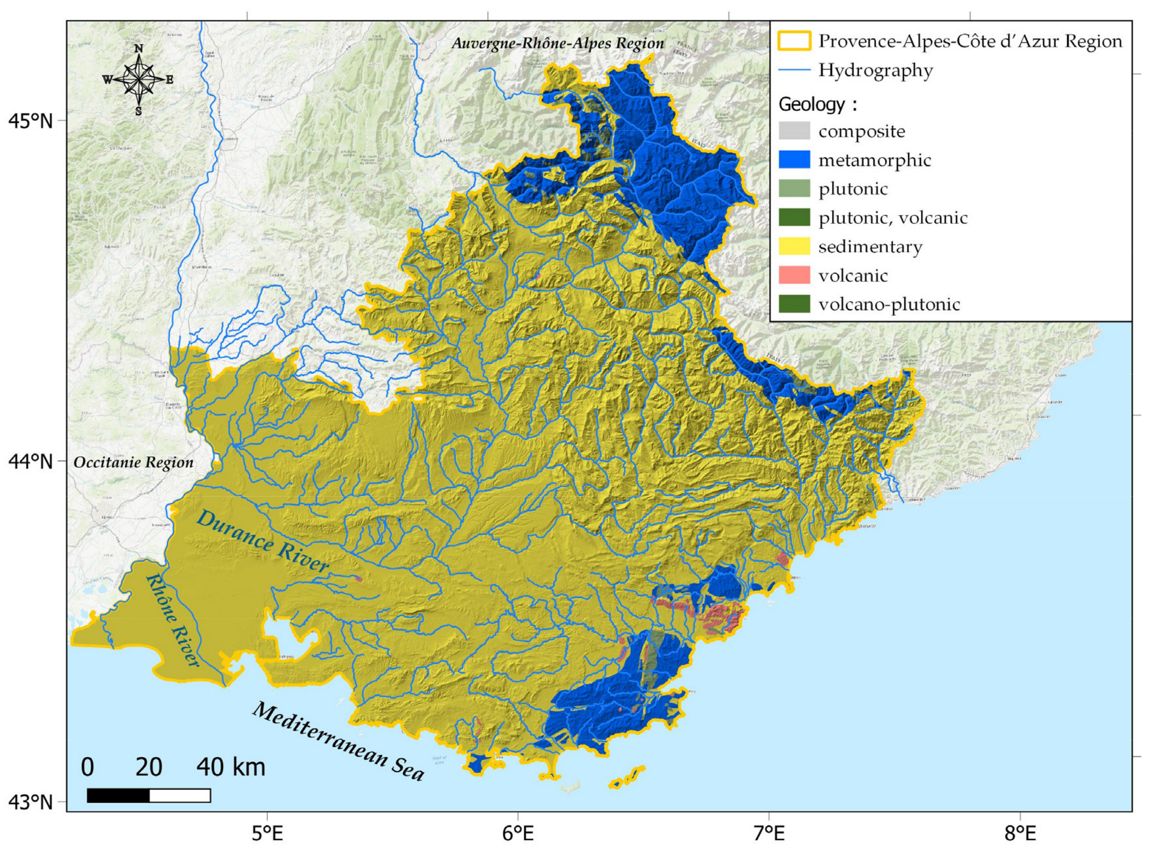
2.1. Study Location

This study was conducted in the Provence-Alpes-Côte d’Azur (PACA) region located in southwestern France (Figure 1). The PACA region, with a surface area of around 31,400 km², is characterized by an important altitudinal gradient, ranging from 0 to 4000 m, and by a diversified geology and lithology (Figure 2), as well as a variety of aquifers (Karstic, sedimentary, of fractured basement or accompanying rivers). The water exploitation index (WEI+), the ratio of total annual water withdrawal to the long-term annual average of renewable freshwater resources, is between 30 and 40% [25]. The Rhône River marks the western limit of the region, while its main tributary, the Durance, crosses the region from east to west. Small coastal rivers (Argens, Var, etc.) turned towards the Mediterranean Sea complete the hydrographic network as shown in Figure 2. The population is of around 5 million inhabitants with a considerable increase during the summer periods. For more details regarding the PACA region, the reader may refer to the work of Tiouiouine et al. [20,22].

2.2. Data Sources and Processing

SISE-EAUX is a groundwater quality database maintained by the French Ministry of Health and its regional and departmental services and is intended for the organized storage of health-related information on water [18,19]. It has been progressively computerized since 1994, but its systematic use as a database has been widely adopted since 2000. The database includes 250,000 control points throughout France, covering both raw (untreated) and distributed (potentially treated) water. The analyses were performed by laboratories that have received the necessary approvals and laboratory quality certifications. The data extraction for this study covered the entire PACA region over a period of 14 years, from 2006 to 2020, and focused specifically on raw water before any treatment for potability. The database includes a total of 1143 georeferenced sampling points, the distribution of which is presented in Figure 1. The data extraction provided 9117 water samples, on which between 4 and 24 parameters were analyzed, resulting in a hollow matrix of 9117 samples on 24 parameters. Afterwards, a data cleansing stage took place, which included removing observations with missing values and parameters that had a limited number of samples, such as thermotolerant coliforms and revivable bacteria at 22 and 37 degrees Celsius, along with total coliforms, which exhibited a data deficiency exceeding 95%. In the end, all parameters with more than 2.5% missing values were eliminated, resulting in a data loss of 5.4% compared to the initial extraction. After this cleaning phase, a full matrix of 8627 observations and 18 parameters was retained, which corresponds to an average of 7.55 analyses per sampling point over the 14 years of data collection. The retained parameters are Enterococcus (Ent.), Escherichia coli (E. coli), electrical conductivity (EC25), potassium (K), sodium (Na), calcium (Ca), magnesium (Mg), chloride (Cl), sulfate (SO₄), hydrogenocarbonates (HCO₃), nitrates (NO₃), fluoride (F), total dissolved solids (TDS), metals which are iron (Fe) and manganese (Mn), and metalloids which are arsenic (As) and bore (B). The pH was transformed into H+ concentration to avoid mixing log and non-log units.

The European Water Framework Directive (Directive 2000/60/EC) [16] launched the Water Information System for Europe, in which groundwater bodies correspond to discrete volumes of groundwater residing in one or more aquifers [26]. In France, their inventory is the responsibility of the water agencies with the support of the French Geological Survey (BRGM) and is now listed in the French Reference System for GWB [27]. GWBs can be based on common attributes such as lithological composition, flow characteristics (confined or unconfined), karst properties, and proximity to coastal regions. The 1143 sampling points in the study were associated with 63 groundwater bodies, which were subsequently grouped into 11 GWB groups according to the procedure outlined by Tiouiouine et al. [20].

2.3. Data Treatement and Multivariate Statististical Analysis

Given the complexity of the ecosystem, a series of statistical techniques were employed to analyze the data, including a logarithmic transformation to alleviate the impact of outliers on the data, a principal component analysis (PCA) [28], hierarchical clustering (AHC) [29], kriging, and analysis of variance (ANOVA) [24] with the fraction of variance unexplained (FVU). These methods were used to optimize the identification of the processes that influence the chemical quality of groundwater bodies (GWB) in the PACA region of France.

2.3.1. Log Transformation

The presence of outliers was detected using the Z score defined by:

Z = |x − M|/σ,

(1)

where x is the measured value for a given parameter, M is the mean, and σ is the standard deviation. Z values greater than 2.5 and 10 are considered outliers, respectively [21]. The presence of outliers, particularly for microbiological parameters, results in a non-symmetric distribution that deviates from normality. A log transformation of the data was applied according to:

y = log10 (x + DL),

(2)

where x denotes the analytical result and DL is the detection limit. The log transformation aims to modify the value scales of the different parameters by dilating the gaps between low values and contracting those between high values [30].

2.3.2. Principal Component Analysis (PCA)

A principal component analysis (PCA) based on the correlation matrix was performed on all parameters [31] in order to reduce the dimensionality of the data space while minimizing the loss of information contained in the dataset. This procedure, based on standardized data centered on the mean and divided by the standard deviation, ensured that each variable had the same weight in the PCA, regardless of the unit used. This method is based on the principle that the resulting factorial axes (principal components) are orthogonal to each other, and therefore carry information related to interdependent processes [32,33].

2.3.3. Hierarchical Clustering

Subsequently, an agglomerative hierarchical clustering (AHC) using the Ward’s linkage method [34,35] was performed using the mean values of each groundwater body on the principal components obtained from the PCA. The relative similarities among the GWB were quantified using Euclidean distance, and the levels of similarity at which the GWB were merged were used to construct a dendrogram.

2.3.4. Spatial and Temporal Variability

In order to measure the amount of information lost when downscaling from catchment to GWB and then to grouping of GWBs, an analysis of variance (ANOVA) was conducted with water characteristics as the dependent variable, and individual catchments, GWBs, and groups of GWBs as categorical explanatory variables [36]. The variance explained by the categorical variable was measured by the R² [37], according to the formula:

R² = 1 − (RSS/TSS),

(3)

where RSS is the residual square sum and TSS is the total square sum. R² denotes the percentage of variation in the response variable that is explained by its relationship with the explanatory variables. As the analyses were carried out at several dates on several sampling points, the variance includes on the one hand the temporal variability, which results in different values on the same sampling point, and on the other hand the spatial variability, which results in different averages between the sampling points. The R² calculated on the criterion “sampling point” as a non-quantitative explanatory variable corresponds to the spatial variability at this scale. The complement to 1 of the R² which is the fraction of variance unexplained (FVU) [38] reflects the temporal variance added to a small part of variance linked to the analytical imprecision, which will be neglected. The same calculation was carried out at the scale of GWBs and groups of GWBs in order to quantify the amount of information contained at these different spatial scales.

2.3.5. Kriging

The spatial structure of each parameter was analyzed by studying the main characteristics of the experimental variograms, such as the range, sill, and nugget effect. The experimental variograms were fitted using spherical models, which were obtained under comparable conditions, (i.e., same number of points and same number of distance classes) [39].

3. Results

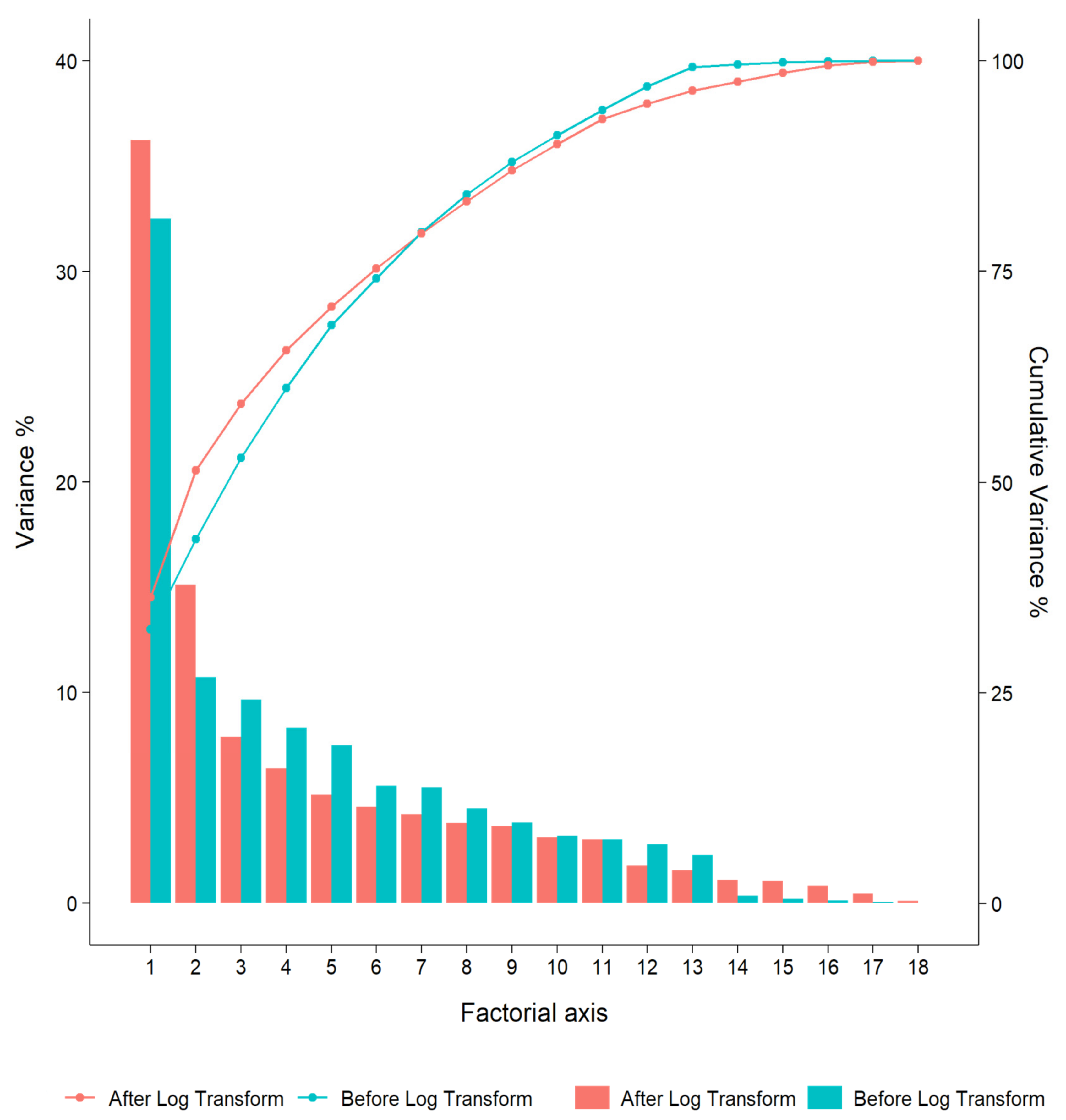
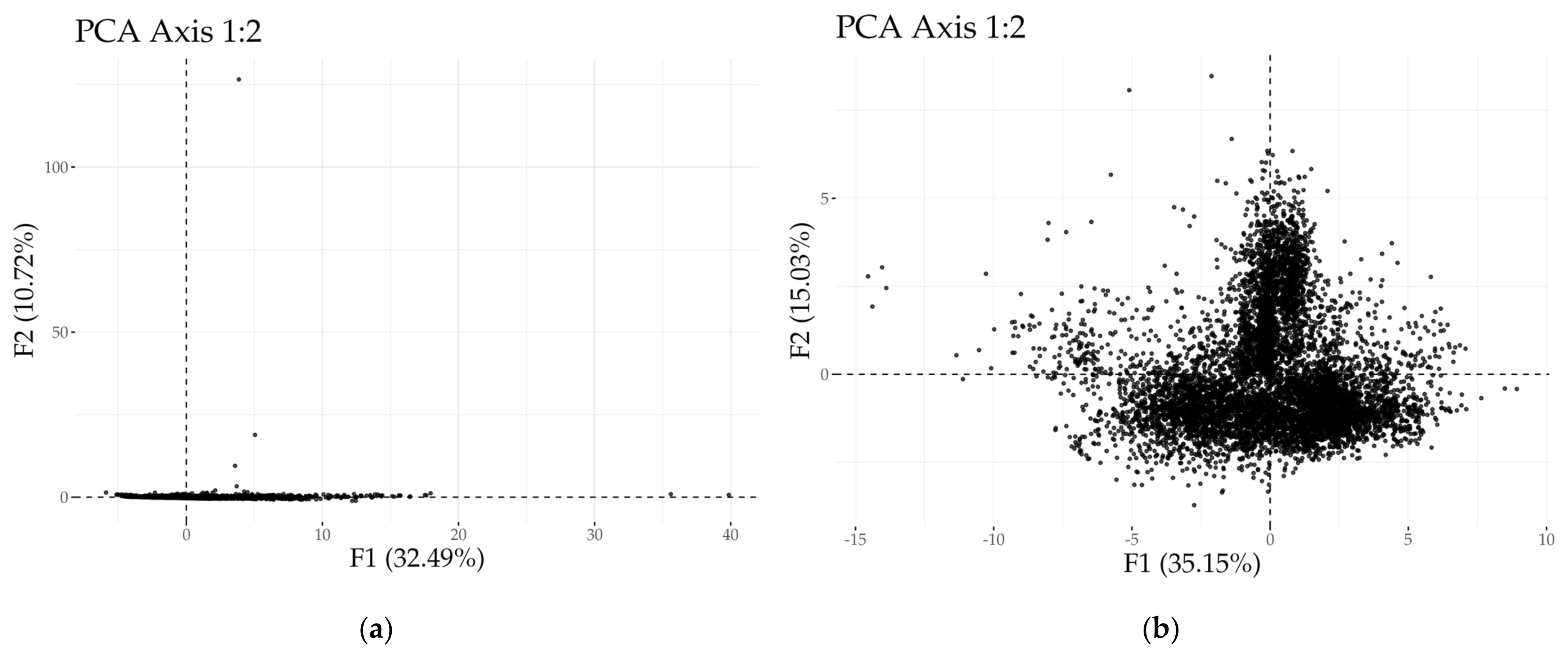
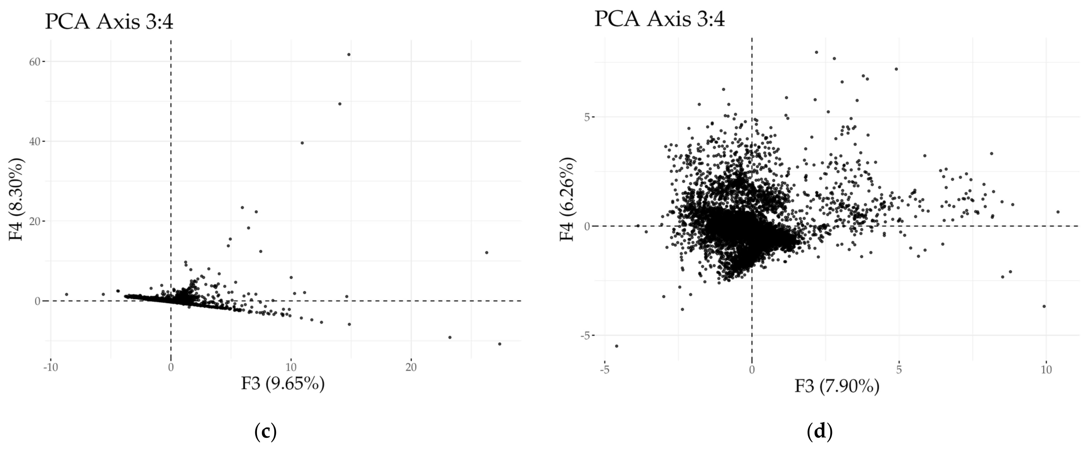
3.1. Achieving a Symmetrical Data Distribution

Figure 3 presents the inertia of the factorial axes of the PCAs conducted on the raw and log-transformed data. The first eight principal components accounted for 85.6% of the total variance for all parameters and all samples combined. Despite the high number of parameters and their heterogeneous nature (bacteriological, major ions, metals, metalloids, etc.), the first factorial plane concentrated a significant part of the information, which was significantly higher after log transformation of the data, shifting from 43.2% (10.7 + 32.5) to 51.4% (36.3 + 15.1). The projection of the samples on the factorial plane F1–F2 and F3–F4 (Figure 3) shows that a few samples significantly increase the area of the score plots, with most observations concentrated in a small area (Figure 4a,c). In contrast, after log transformation of the data, the dispersion of observations in the score plots is more uniform (Figure 4b,d). Therefore, in the following, we will consider the log-transformed data.

3.2. PCA Results: General Chemistry and Spatial Distribution of Groundwater

The first factorial axis (F1) in

Table 1. Contribution of the parameters to the first five factorial axes (PCA with log-transformed data).

	F1	F2	F3	F4	F5
Enterococcus	0.035	0.800	−0.299	−0.241	0.208
E. coli	0.052	0.799	−0.283	−0.244	0.219
K	0.727	0.336	0.230	0.002	−0.267
Na	0.721	0.392	0.202	0.019	−0.305
Ca	0.829	−0.283	−0.299	−0.002	0.094
Mg	0.723	−0.015	−0.061	0.116	0.051
Cl	0.751	0.344	0.161	−0.006	−0.292
SO4	0.729	0.238	0.144	0.042	−0.067
HCO3	0.676	−0.420	−0.402	0.011	0.128
EC25	0.779	−0.129	−0.215	0.066	−0.012
TDS	0.912	−0.226	−0.249	0.045	0.060
pH	−0.378	0.531	−0.189	−0.224	−0.151
Fe	0.070	0.423	−0.109	0.663	−0.167
Mn	0.117	0.380	−0.017	0.541	0.524
As	−0.199	0.074	0.619	0.229	0.219
NO3	0.531	−0.200	0.245	−0.185	0.079
B	0.554	0.048	0.285	−0.196	0.254
F	0.522	0.055	0.415	−0.277	0.325

Note(s): ^Bold Parameter contribution in the factorial axis of (+/−) 0.7.

contrasted mineralized water without fecal contamination with diluted water contaminated by E. coli and Enterococcus. This is notably highlighted by high variable contributions (above 0.7) in the majority of major ions, TDS, and electrical conductivity in F1. We assert clearly that this is an axis of water mineral load. The second factorial axis (F2) was mainly scored with waters contaminated by fecal bacteria with E. coli. and Enterococcus having scored around 0.8. Contaminated waters were rather reductive as shown by the positive coordinates of metals and negative of nitrates. The third factorial axis reflected mainly waters with the highest arsenic, nitrate, fluorine, and boron content, and the fourth factorial axis reflected redox processes, but for waters with low contamination by fecal bacteria.

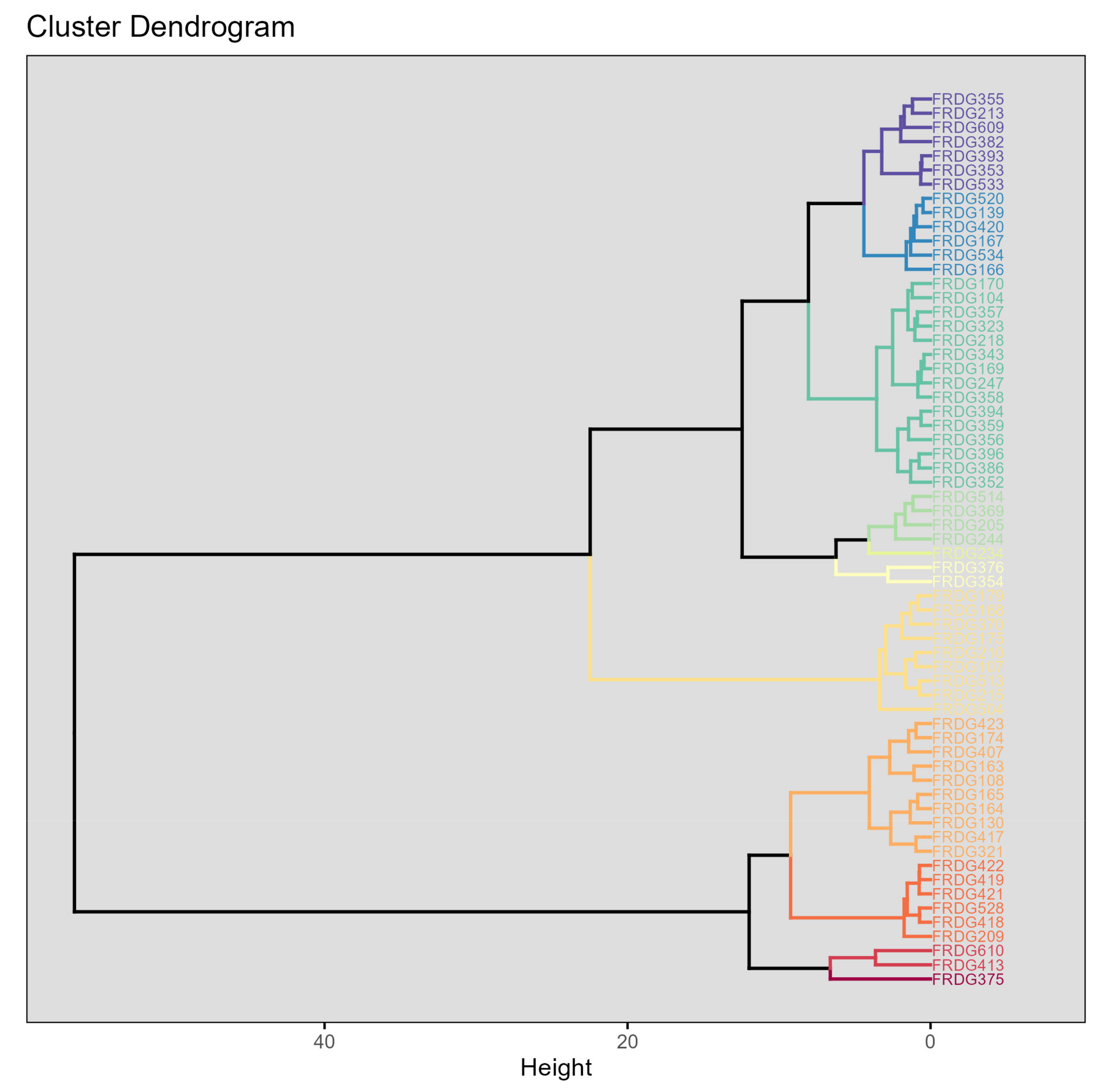
3.3. AHC Results: Grouping Groundwater Bodies Using AHC

The clustering of GWBs based on their average coordinates on the first 10 factorial axes is presented in Figure 5, where 11 distinct groups were identified. The mapping of these 11 groups is presented in Figure 6. A strong correlation was observed between the GWB groups and the regional geology and geomorphology. For example, group 9 represents all the accompanying water tables of the hydrographic network, group 11 corresponds to low altitude discontinuous aquifers (karst and fractured aquifers), group 6 groups together sedimentary coastal aquifers, and group 1 identifies high altitude fractured aquifers in crystalline bedrocks.

Figure 6 below shows the main spatial distribution of GWB body group. The main visually observed remark from this clustering is the resemblance between some clusters and the lithological limit. Cluster 1 is located within the coastal crystalline group, cluster 2 corresponds to the alpine crystalline group, clusters 3 and 4 are located within the sedimentary ensembles in altitude, group 5 is exclusive to the sedimentary rocks within the coastal south to southwest PACA, group 9 is located within the alluvial plains of the Rhone and Durance rivers, group 10 is located also in the sedimentary formations near the alluvial plains, and group 11 is located within two formations, the crystalline coastal formations and near the alluvial plains in the Durance river.

The clustering of GWBs based on their average coordinates on the first 10 factorial axes is presented in Figure 5, where 11 distinct groups were identified. The mapping of these 11 groups is presented in Figure 6. A strong correspondence was observed between GWB groups and regional geology and geomorphology.

Groups 1 and 2 are located in the coastal and alpine crystalline contexts, respectively. Groups 3 and 4 are located in the sedimentary complexes at high altitude and group 5 is exclusive to the sedimentary rocks of the south to southwest coast of the PACA region. Groups 6, 7, and 8 are small and isolated. Group 9 is located in the alluvial plains of the Rhone and Durance rivers and includes all the water tables accompanying the hydrographic network. Group 10 is situated in the sedimentary formations close to the alluvial plains, and group 11 is situated in two formations, the coastal crystalline formations and close to the alluvial plains of the Durance river, which are discontinuous aquifers of low altitude (karst and fractured environments).

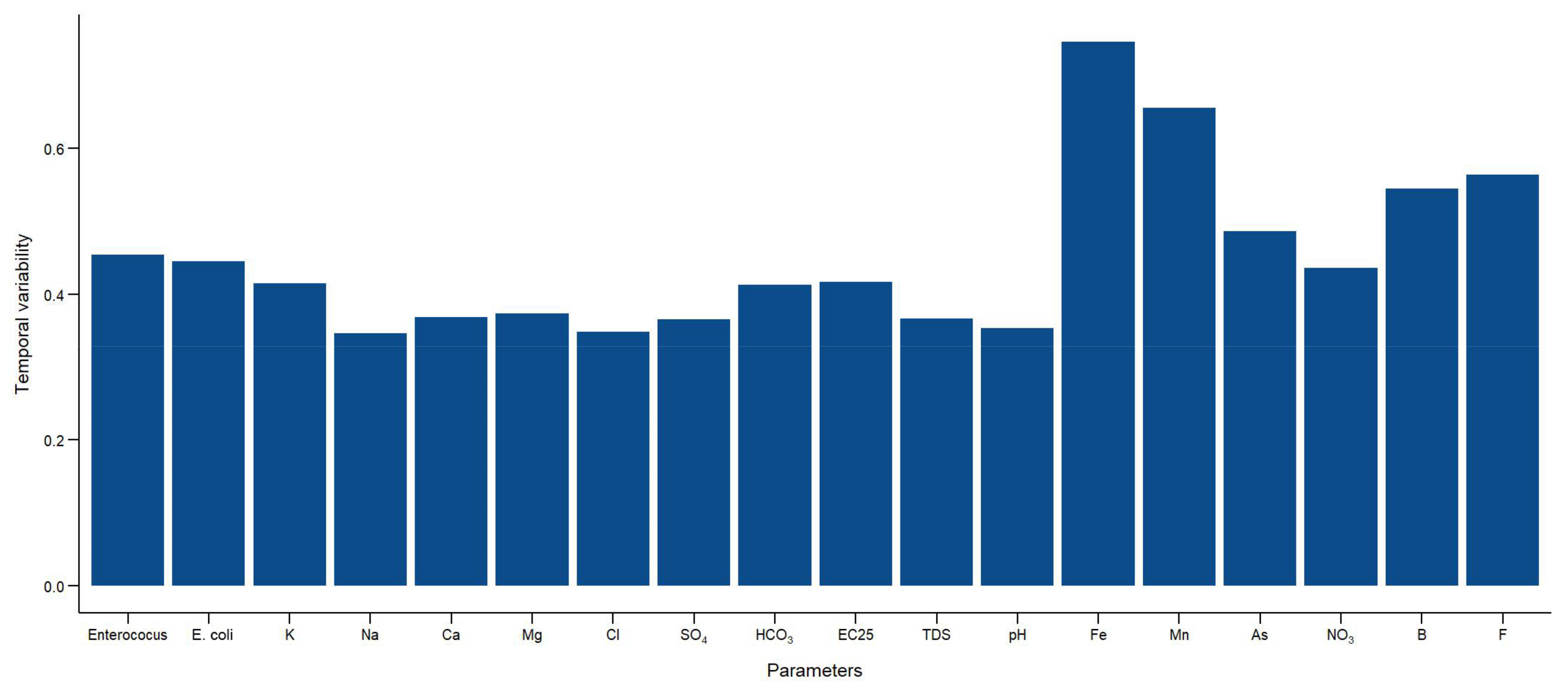
3.4. Spatial and Temporal Variability

Table 2. Adjusted special variogram parameters and ANOVA R² for Enterococcus, E. coli, electrical conductivity 25°, and sodium.

Parameter	Nugget	Spherical Semi-Variance	Lag	% Nugget Effect	ANOVA R2
Enterococcus	0.28	0.12	4000	70.0	0.546
E. coli	0.3	0.22	3000	57.7	0.555
EC25	0.007	0.042	62,000	14.3	0.654
Na	0.08	0.36	150,000	18.2	0.583

summarizes the main characteristics of the variograms obtained for some key parameters (bacteriology and major ions). A significant nugget effect was observed for the bacteriological parameters, combined with a very small range, of the order of a few km. On the other hand, the nugget effect is practically null for electrical conductivity and major ions (represented here by sodium), with a high range of several tens of km.

The temporal variability evaluated by the R² for each parameter is presented in Figure 7. This was high for metals with values reaching 65 to 70%, close to 55 to 60% for trace elements F, B, and As, around 45% for bacteriological parameters, but generally below 40% for major ions.

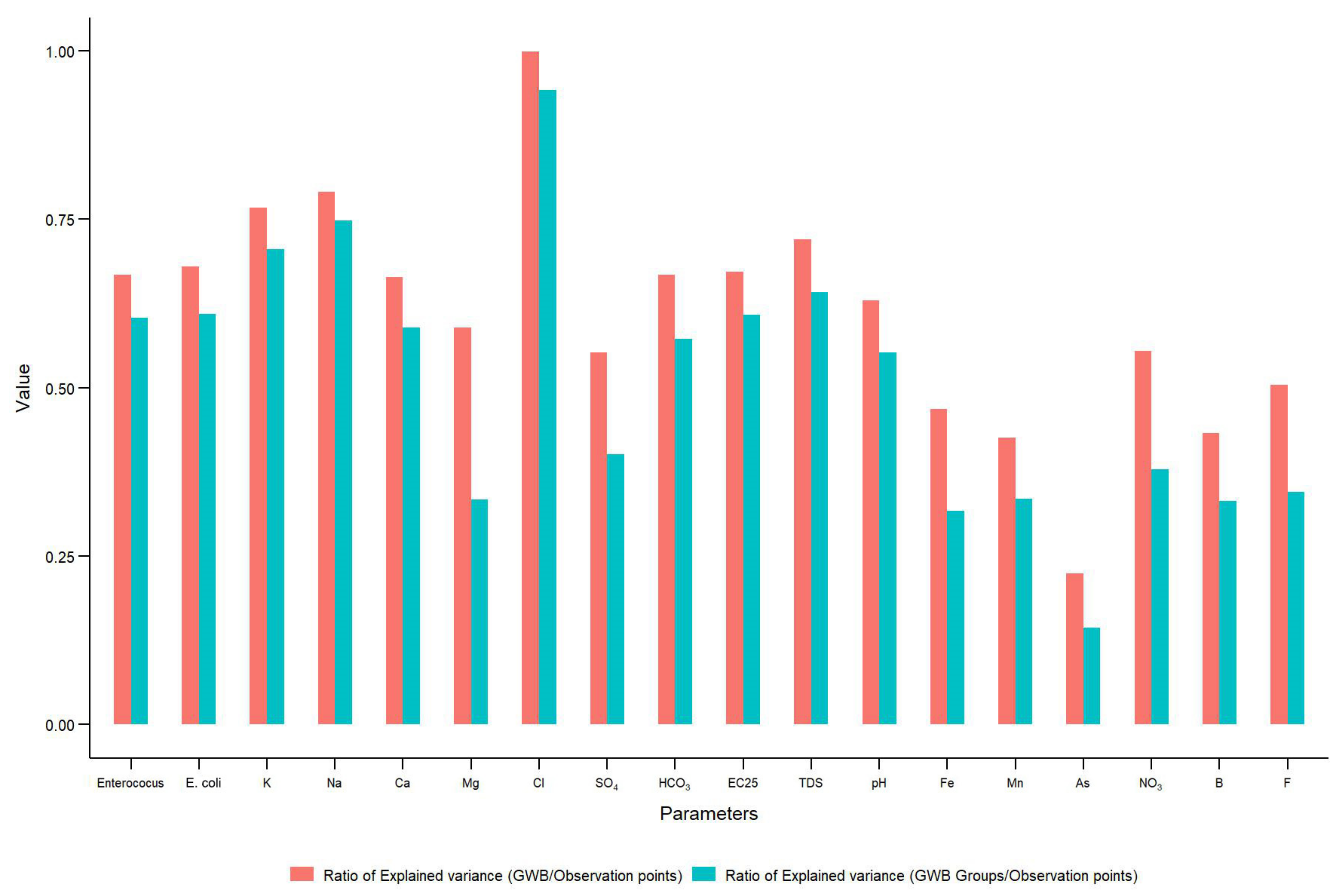
3.5. Determining the Proper Scaling of Groundwater Water Quality

The ratios of variance explained in the two groupings, namely from the scale of collection points to the GWBs and then from GWBs to GWB groups, is presented in Figure 8. In the first aggregation, most of the major ions show a moderate decrease (between 0.7 and 0.99), except for Mg and SO4 ions whose ratio showed a decrease of about 0.6. For nitrates, the ratio was also around 0.6. The ratio for bacteriological parameters showed a moderate decrease (0.55) in spatial variation, while metals and other trace elements showed a decrease in the range of 0.5 to 0.25. At the second aggregation, these ratios decreased slightly on the order of 0.1.

4. Discussion

4.1. Processes of Acquisition of Water Characteristics

The logarithmic transformation of the data clearly allows limiting the weight of outliers, mainly observed for bacteriological parameters. This transformation, already tested on other similar databases [21], allows a stronger concentration of information on the first factorial axes and facilitates the interpretation of the associated processes. The logarithmic transformation of the data also reduces the temporal variability of some parameters, especially bacteriological parameters, a point that will be analyzed in the next paragraph. Minerality is the main factor of variability in the waters of the PACA region. This point has already been emphasized by several studies conducted in the region, whether it is the work of Tiouiouine [20] on which we have relied, or other works conducted in more targeted environments. Thus, minerality is the main factor of water variability within the karst system of Fontaine de Vaucluse and is even identified as a major factor of flow discrimination within the karst [40]. Minerality is also frequently identified as a major variability factor among surface waters on all continents [41]. The second factor of variability in water quality is bacterial contamination, which more specifically affects waters with low mineralization. This is again a classic phenomenon in Mediterranean environments, where late summer storms cause runoff of low mineralized water but with high turbidity and likely to carry a high bacterial load. These waters infiltrate as they flow through the watersheds and contaminate the groundwater. The second factorial axis represents a spatial opposition between mineralized waters with a calcareous carbonate chemical profile and non-carbonate waters that are less mineralized but reductive (attested by the presence of soluble metals) and contaminated by bacteria. The fecal contamination of calcareous, mineralized, and reducing waters appears as the next factor. It can be interpreted as a contrast between more or less old waters in karst environments (i.e., with a higher residence time and which are generally discriminated by higher magnesium contents) [42,43]. Thus, PCA reveals several distinct signatures of fecal contamination, which are represented by distinct factorial axes. There is thus a diversity of situations and mechanisms related to this contamination, as mentioned by Tiouiouine et al. [22]. The mechanisms leading to fecal contamination are not solely limited to surface transport during storm events infiltrating susceptible water catchments, even though this is the most common scenario.

4.2. A Relevant and Efficient Grouping of GWBs

The implementation of a groundwater protection and monitoring policy by health agencies cannot be done on the scale of too many catchment points. A relevant grouping, in homogeneous sets and in coherence with the physicochemical and bacteriological characteristics, is necessary. The knowledge of which catchment points belong to a given GWB is an independent and essential source of information that must obviously be taken into consideration, but the number, 63 in the PACA region and 106 in the neighboring Occitanie region [21], is still too high to implement specific recommendations for each GWB. The reduction in the fineness of description of the information contained in the 8627 water samples collected is drastic when going from 1143 to 63 and then to 11 spatial units (i.e., from sampling points to GWBs and then to groups of GWBs).

The calculation of temporal variability is based on the calculation of R² when moving from 8627 collected water samples to 1143 sample points, which resulted in a reduction in the number of data by a factor of 7.5. Temporal variability can also be estimated by the nugget effect observed on the variograms which appears as variance for zero distance, with samples collected from the same point on multiple dates. The comparison between R² (Figure 7) and nugget effect for each parameter confirms this. The temporal variability is important, of the order of a third or more of the total variability, less for the chemistry of major ions than for trace elements or bacteriological parameters. In the transition from the observation point scale to the GWB scale, factors that explain changes in variance include differences in borehole characteristics (such as wells or springs), differences in borehole vulnerability, and heterogeneity of land use in the vicinity of boreholes. The difference in explained variance between groups of GWBs is mainly related to differences in geological characteristics between GWBs. The rates of spatial variability and loss of information during upscaling have different values for different parameters, which can be explained by the diversity of transport mechanisms for these parameters. For bacteriological parameters, the transport of particle fixed bacteria is limited by the pore size, while they enter the boreholes by contamination of runoff water. This leads to a high temporal variability of their concentrations, which can be very sensitive to precipitation events. In general terms, this typology of parameters’ behavior is strongly correlated to the spatial structure. Indeed, the parameters that show greater temporal variability are also those that show local spatial variability (Table 2). Thus, there appears to exist a relationship between the local character of spatial variation and the intensity of temporal variability. This constitutes a first basis for a typology of microbiological and physicochemical parameters, which will be the subject of a future publication.

As with temporal variability, the log transformation preserves a greater proportion of the information contained in the dataset. With raw data, almost all spatial information is lost for bacteriological parameters when grouping from catchment points to GWBs and then to GWB groups. The difference is significant and the lack of data conditioning would be detrimental to the methodology. In this sense, this work considerably improves the results previously presented by Tiouiouine [20] in the same PACA region. The loss of spatial information that accompanies the two aggregations varies according to the parameter. For chlorides, the loss is minimal, and the aggregation into GWB groups preserves more than 90% of the initial spatial information. For sodium, electrical conductivity, and E. coli content, more than half of the spatial information is preserved at the GWB group level, with most of the information loss occurring during the first aggregation of the sample points to the corresponding GWBs. For elements with high local variability such as Fe, Mn, and NO3, the loss of information is more important, but about 30–40% of the spatial information is still preserved by the GWB groups. Again, as for the other parameters, the switch from GWBs to GWB groups causes only a minor part of the information loss, the bulk being lost during the first aggregation.

4.3. Methodological Contributions

The present work highlights a series of methodological advances that we feel are relevant to bring together here:

• The log transformation to the data greatly reduces the problem of data non-normality and improves the statistical properties of the dataset, thus enhancing the robustness and reliability of subsequent analyses.
• It also mitigates the effects of outliers without eliminating the information they convey. The integrity of the dataset is thus preserved for analysis.
• The quantification of the loss of information that accompanies the clustering allows the effectiveness of the method to be measured.
• However, the proposed method has certain limitations. In particular, at this stage, the analysis is carried out parameter by parameter, which does not take into account the interrelations between several parameters. A more integrated approach, which could be based on principal components rather than on parameters, could be developed, but it would go beyond the scope of our study. It should be noted, however, that this approach is implicitly supported by the generation of GWB groups, as the classification process takes into account the relationships between different groundwater quality parameters.
• The method applied here is currently being applied in parallel in other French administrative regions and should be the subject of further advances. Whether the groundwater conditions are similar or quite different, there is no reason why the analysis should not be similar to the one conducted here. This method is flexible and applicable to various geological contexts and hydrogeological conditions. The applicability depends on the availability of a statistically significant number of samples per observation point and per GWB. Interpretation will, of course, be guided by the specificities of the region under consideration in terms of geological formations, land use patterns, and possible sources of contamination.

5. Conclusions

The objective of this work was to quantify the spatial variability and temporal variability of the multiparameter quality of groundwater in a region, and to measure the loss of information when implementing the upscaling method proposed by Tiouiouine et al. [20]. This method consists in reducing the dimensionality of the data by PCA, then classifying the groundwater bodies into homogeneous groups according to the average values by GWB.

The analysis of variance shows that the share of temporal variability in the total variance depends strongly on the nature of the quality parameters. The temporal variability is higher for microbiological parameters, and less important for major ions. The analysis of variance made it possible to quantify the loss of information inherent to the grouping and the decrease in the number of units from 1143 sampling points to 63 GWB and then to 11 GWB groups. The amount of information lost also varies according to the quality parameter considered.

The monitoring of water quality for human consumption is the responsibility of the health agencies. The number of 11 homogeneous groups is suitable for the development of a specific roadmap and targeted recommendations for each group of GWB. More specifically, for the PACA region, the detailed analysis of each group will be the next step in our research schedule.

References

- Jakeman, A.J.; Barreteau, O.; Hunt, R.J.; Rinaudo, J.-D.; Ross, A.; Arshad, M.; Hamilton, S. Integrated Groundwater Management: An Overview of Concepts and Challenges. In Integrated Groundwater Management; Springer: Berlin/Heidelberg, Germany, 2016; pp. 3–20. [Google Scholar]
- Priyan, K. Issues and Challenges of Groundwater and Surface Water Management in Semi-Arid Regions. In Groundwater Resources Development and Planning in the Semi-Arid Region; Springer: Berlin/Heidelberg, Germany, 2021; pp. 1–17. [Google Scholar]
- Syafiuddin, A.; Boopathy, R.; Hadibarata, T. Challenges and Solutions for Sustainable Groundwater Usage: Pollution Control and Integrated Management. Curr. Pollut. Rep. 2020, 6, 310–327. [Google Scholar] [CrossRef]
- Foster, S. Global Policy Overview of Groundwater in Urban Development—A Tale of 10 Cities! Water 2020, 12, 456. [Google Scholar] [CrossRef]
- Closas, A.; Villholth, K.G. Groundwater Governance: Addressing Core Concepts and Challenges. WIREs Water 2020, 7, e1392. [Google Scholar] [CrossRef]
- Walker, D.B.; Baumgartner, D.J.; Gerba, C.P.; Fitzsimmons, K. Surface Water Pollution. In Environmental and Pollution Science; Elsevier: Amsterdam, The Netherlands, 2019; pp. 261–292. [Google Scholar]
- Li, P.; Karunanidhi, D.; Subramani, T.; Srinivasamoorthy, K. Sources and Consequences of Groundwater Contamination. Arch. Environ. Contam. Toxicol. 2021, 80, 1–10. [Google Scholar] [CrossRef] [PubMed]
- Daly, D. Groundwater—The ’hidden Resource’. In Proceedings of the Biology and Environment: Proceedings of the Royal Irish Academy; Royal Irish Academy: Dublin, Ireland, 2009; Volume 109, pp. 221–236. [Google Scholar]
- Koundouri, P. Current Issues in the Economics of Groundwater Resource Management. J. Econ. Surv. 2004, 18, 703–740. [Google Scholar] [CrossRef]
- Kemper, K.E. Groundwater—From Development to Management. Hydrogeol. J. 2004, 12, 3–5. [Google Scholar] [CrossRef]
- Ortiz-Letechipia, J.; González-Trinidad, J.; Júnez-Ferreira, H.E.; Bautista-Capetillo, C.; Dávila-Hernández, S. Evaluation of Groundwater Quality for Human Consumption and Irrigation in Relation to Arsenic Concentration in Flow Systems in a Semi-Arid Mexican Region. Int. J. Environ. Res. Public Health 2021, 18, 8045. [Google Scholar] [CrossRef] [PubMed]
- Chave, P. The EU Water Framework Directive; IWA Publishing: London, UK, 2001; ISBN 1900222124. [Google Scholar]
- Kallis, G.; Butler, D. The EU Water Framework Directive: Measures and Implications. Water Policy 2001, 3, 125–142. [Google Scholar] [CrossRef]
- European Commission. Directive 2014/80/EU Amending Annex II to Directive 2006/ 118/EC of the European Parliament and of the Council on the Protection of Groundwater Against Pollution and Deterioration. Off. J. Eur. Union 2014, L182, 52–55. [Google Scholar]
- European Commission. Directive 2006/118/EC of the European Parliament and of the Council of 12 December 2006 on the Protection of Groundwater against Pollution and Deterioration. Off. J. Eur. Union 2006, 19–31. Available online: https://eur-lex.europa.eu/legal-content/EN/TXT/?uri=celex%3A32006L0118 (accessed on 21 January 2023).
- European Commission. Directive 2000/60/EC of the European Parliament and of the Council of 23 October 2000 Establishing a Framework for Community Action in the Field of Water Policy. Off. J. Eur. Communities 2000, L327, 1–72. [Google Scholar]
- Brugeron, A. Cartographie et Systèmes d’Information Géographique Pour La Gestion Des Ressources En Eau Souterraine; HAL: Paris, France, 2012. [Google Scholar]
- Pouey, J.; Galey, C.; Chesneau, J.; Jones, G.; Franques, N.; Beaudeau, P. EpiGEH, groupe des référents régionaux; Mouly, D. Implementation of a National Waterborne Disease Outbreak Surveillance System: Overview and Preliminary Results, France, 2010 to 2019. Eurosurveillance 2021, 26, 2001466. [Google Scholar] [CrossRef] [PubMed]
- Beaudeau, P.; Pascal, M.; Mouly, D.; Galey, C.; Thomas, O. Health Risks Associated with Drinking Water in a Context of Climate Change in France: A Review of Surveillance Requirements. J. Water Clim. Chang. 2011, 2, 230–246. [Google Scholar] [CrossRef]
- Tiouiouine, A.; Jabrane, M.; Kacimi, I.; Morarech, M.; Bouramtane, T.; Bahaj, T.; Yameogo, S.; Rezende-Filho, A.T.; Dassonville, F.; Moulin, M.; et al. Determining the Relevant Scale to Analyze the Quality of Regional Groundwater Resources While Combining Groundwater Bodies, Physicochemical and Biological Databases in Southeastern France. Water 2020, 12, 3476. [Google Scholar] [CrossRef]
- Jabrane, M.; Touiouine, A.; Bouabdli, A.; Chakiri, S.; Mohsine, I.; Valles, V.; Barbiero, L. Data Conditioning Modes for the Study of Groundwater Resource Quality Using a Large Physico-Chemical and Bacteriological Database, Occitanie Region, France. Water 2023, 15, 84. [Google Scholar] [CrossRef]
- Tiouiouine, A.; Yameogo, S.; Valles, V.; Barbiero, L.; Dassonville, F.; Moulin, M.; Bouramtane, T.; Bahaj, T.; Morarech, M.; Kacimi, I. Dimension Reduction and Analysis of a 10-Year Physicochemical and Biological Water Database Applied to Water Resources Intended for Human Consumption in the Provence-Alpes-Cote d’azur Region, France. Water 2020, 12, 525. [Google Scholar] [CrossRef]
- Ozer, D.J. Correlation and the Coefficient of Determination. Psychol. Bull. 1985, 97, 307. [Google Scholar] [CrossRef]
- St, L.; Wold, S. Analysis of Variance (ANOVA). Chemom. Intell. Lab. Syst. 1989, 6, 259–272. [Google Scholar]
- Psomas, A.; Bariamis, G.; Roy, S.; Rouillard, J.; Stein, U. Comparative Study on Quantitative and Chemical Status of Groundwater Bodies: Study of the Impacts of Pressures on Groundwater in Europe, Service Contract, 315/B2020/EEA.58185; EEA: Copenhagen, Denmark, 2021. [Google Scholar]
- Maréchal, J.-C.; Rouillard, J. Groundwater in France: Resources, Use and Management Issues. In Sustainable Groundwater Management: A Comparative Analysis of French and Australian Policies and Implications to Other Countries; Springer: Berlin/Heidelberg, Germany, 2020; pp. 17–45. [Google Scholar]
- Masses d’eau Souterraines-Métropole-Version État Des Lieux 2019. Available online: https://geo.data.gouv.fr/fr/datasets/1a983edfe5ea441fef359a652e98217c9c3ce3c6 (accessed on 20 March 2021).
- Ringnér, M. What Is Principal Component Analysis? Nat. Biotechnol. 2008, 26, 303–304. [Google Scholar] [CrossRef]
- Madhulatha, T.S. An Overview on Clustering Methods. arXiv 2012, arXiv:1205.1117. [Google Scholar] [CrossRef]
- Cousineau, D.; Chartier, S. Outliers Detection and Treatment: A Review. Int. J. Psychol. Res. 2010, 3, 58–67. [Google Scholar] [CrossRef]
- Pearson, K. On Lines and Planes of Closest Fit to Systems of Points in Space. Lond. Edinb. Dublin Philos. Mag. J. Sci. 1901, 2, 559–572. [Google Scholar] [CrossRef]
- Helena, B.; Pardo, R.; Vega, M.; Barrado, E.; Fernandez, J.M.; Fernandez, L. Temporal Evolution of Groundwater Composition in an Alluvial Aquifer (Pisuerga River, Spain) by Principal Component Analysis. Water Res. 2000, 34, 807–816. [Google Scholar] [CrossRef]
- Rezende-Filho, A.T.; Valles, V.; Furian, S.; Oliveira, C.M.S.C.; Ouardi, J.; Barbiero, L. Impacts of Lithological and Anthropogenic Factors Affecting Water Chemistry in the Upper Paraguay River Basin. J. Environ. Qual. 2015, 44, 1832–1842. [Google Scholar] [CrossRef] [PubMed]
- Day, W.H.E.; Edelsbrunner, H. Efficient Algorithms for Agglomerative Hierarchical Clustering Methods. J. Classif. 1984, 1, 7–24. [Google Scholar] [CrossRef]
- Bouguettaya, A.; Yu, Q.; Liu, X.; Zhou, X.; Song, A. Efficient Agglomerative Hierarchical Clustering. Expert Syst. Appl. 2015, 42, 2785–2797. [Google Scholar] [CrossRef]
- Owamah, H.I. A Comprehensive Assessment of Groundwater Quality for Drinking Purpose in a Nigerian Rural Niger Delta Community. Groundw. Sustain. Dev. 2020, 10, 100286. [Google Scholar] [CrossRef]
- Miles, J. R-Squared, Adjusted R-Squared. In Encyclopedia of Statistics in Behavioral Science; R Foundation for Statistical Computing: Vienna, Austria, 2005; ISBN 9780470013199. [Google Scholar]
- Achen, C.H. What Does “Explained Variance“ Explain?: Reply. Political Anal. 1990, 2, 173–184. [Google Scholar] [CrossRef]
- Cressie, N. The Origins of Kriging. Math. Geol. 1990, 22, 239–252. [Google Scholar] [CrossRef]
- Barbel-Périneau, A.; Barbiero, L.; Danquigny, C.; Emblanch, C.; Mazzilli, N.; Babic, M.; Simler, R.; Valles, V. Karst Flow Processes Explored through Analysis of Long-Term Unsaturated-Zone Discharge Hydrochemistry: A 10-Year Study in Rustrel, France. Hydrogeol. J. 2019, 27, 1711–1723. [Google Scholar] [CrossRef]
- Rezende Filho, A.T.; Furian, S.; Victoria, R.L.; Mascré, C.; Valles, V.; Barbiero, L. Hydrochemical Variability at the Upper Paraguay Basin and Pantanal Wetland. Hydrol. Earth Syst. Sci. 2012, 16, 2723–2737. [Google Scholar] [CrossRef]
- Batiot, C.; Emblanch, C.; Blavoux, B. Total Organic Carbon (TOC) and Magnesium (Mg2+): Two Complementary Tracers of Residence Time in Karstic Systems. Comptes Rendus Geosci. 2003, 335, 205–214. [Google Scholar] [CrossRef]
- Moral, F.; Cruz-Sanjulián, J.J.; Olías, M. Geochemical Evolution of Groundwater in the Carbonate Aquifers of Sierra de Segura (Betic Cordillera, Southern Spain). J. Hydrol. 2008, 360, 281–296. [Google Scholar] [CrossRef]