
Assessing the Effectiveness of the Use of the InVEST Annual Water Yield Model for the Rivers of Colombia: A Case Study of the Meta River Basin
 , ,
, , 
Abstract
:1. Introduction
2. Materials and Methods
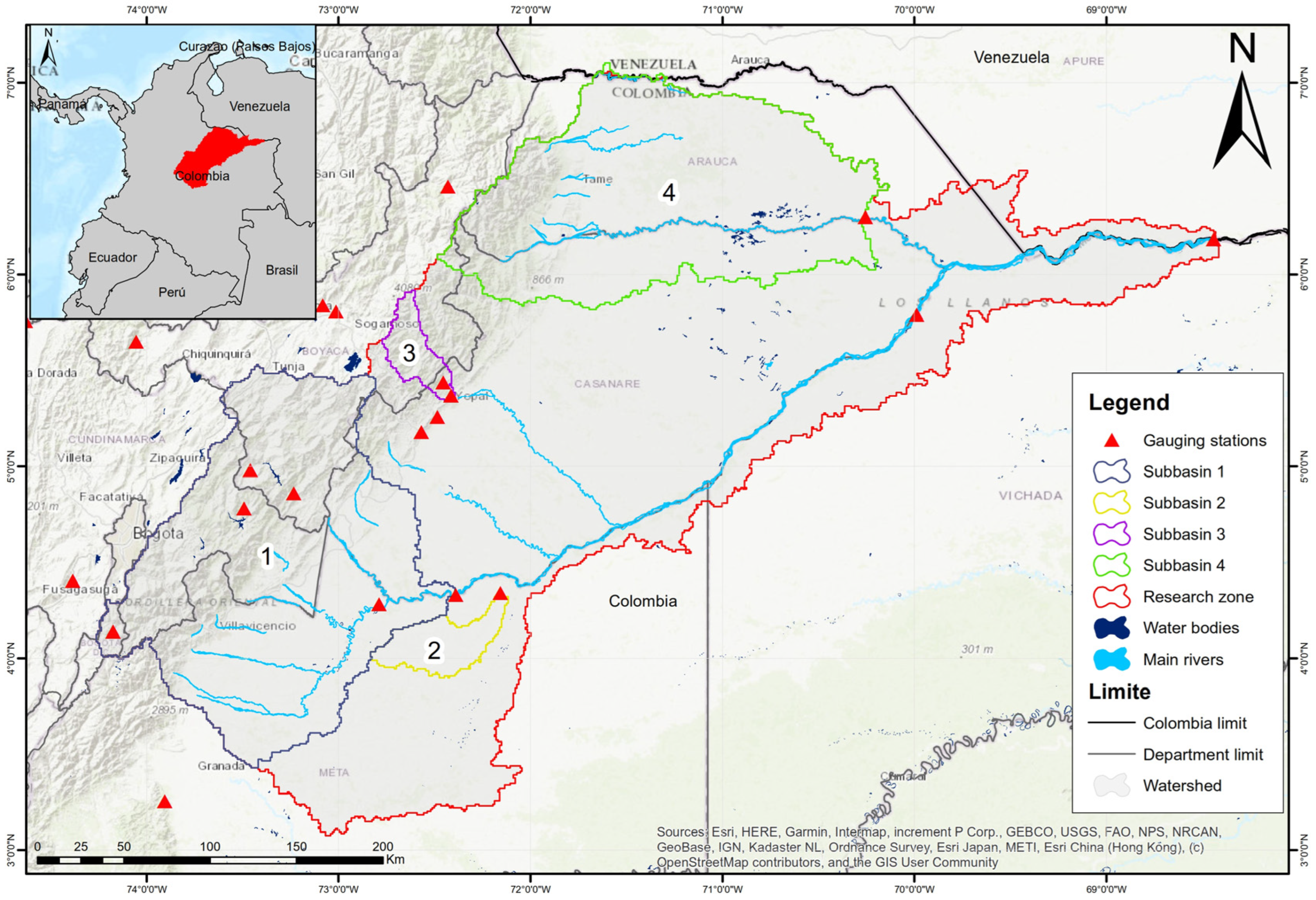
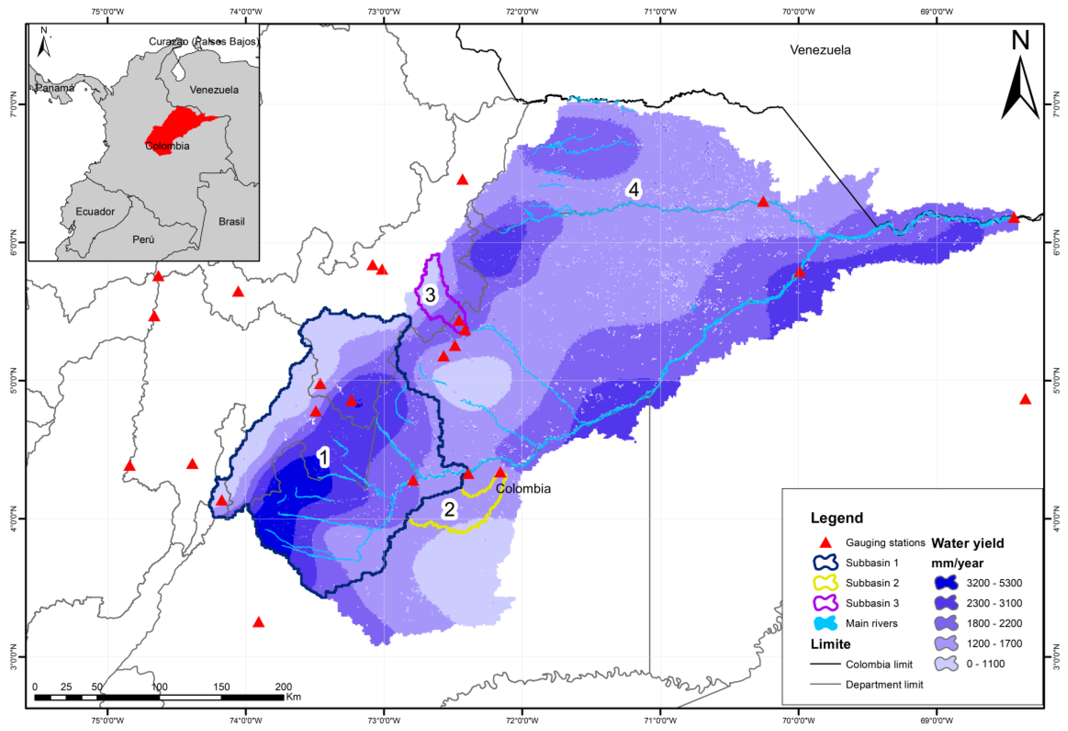
2.1. Study Area
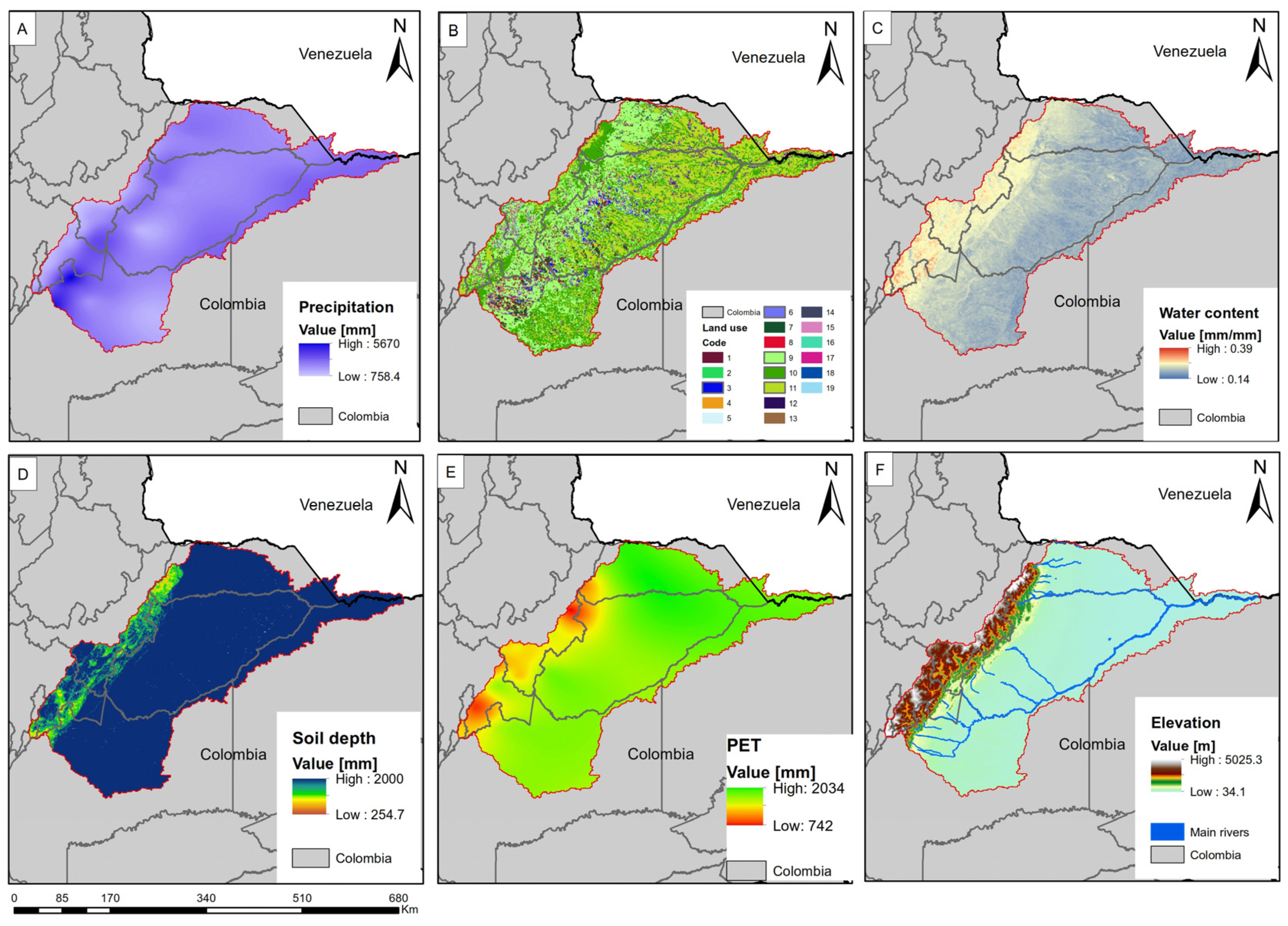
2.2. Materials
2.2.1. Data Requirement
2.2.2. Meteorological Data
2.2.3. Soil Data
2.2.4. Land Use/Land Cover Data and Kc
2.2.5. Water Discharge Data
2.2.6. Zhang Coefficient
2.2.7. The InVEST–AWY Model
2.3. Methods
2.3.1. Methodology
2.3.2. Sensitivity Analysis
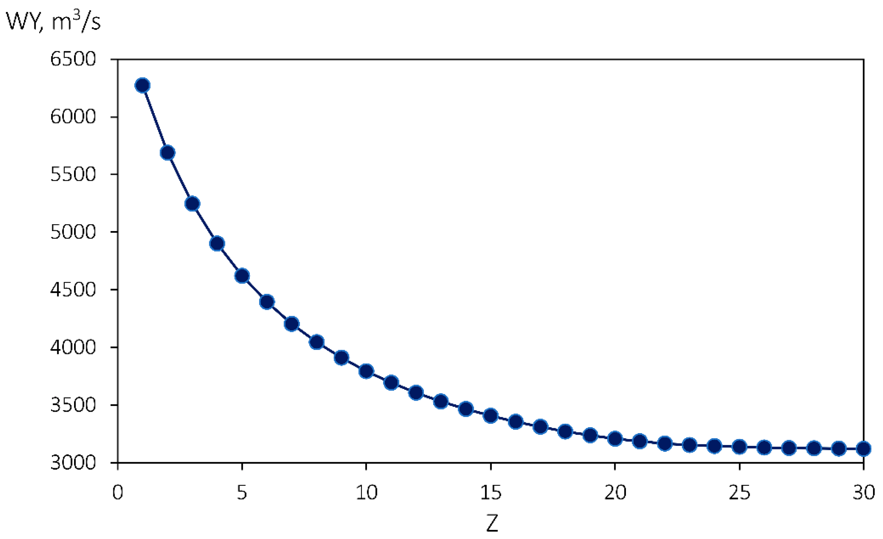
Model Sensitivity to Z
Model Sensitivity to Kc
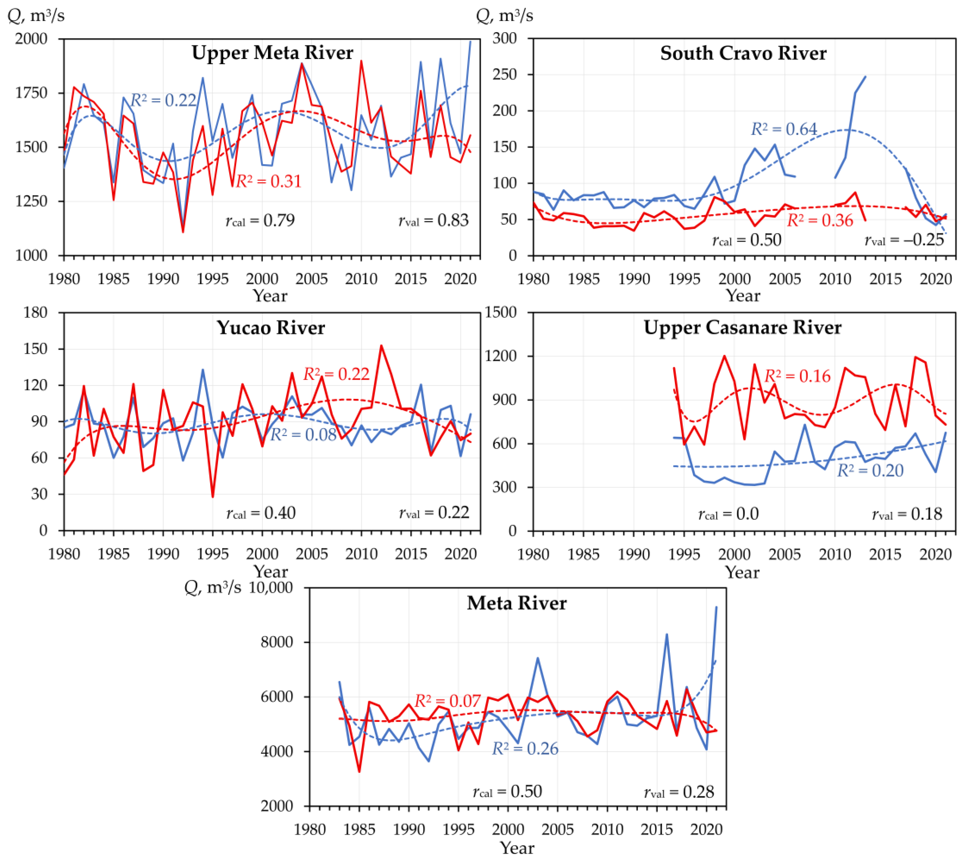
2.3.3. Calibration and Validation
3. Results, Discussion, and Limitations
3.1. Water Yield Formation
3.2. Limitations
3.2.1. Model Limitations
3.2.2. Uncertainties from In-Situ Data
3.2.3. Human Effect on Water Discharge
4. Conclusions
Author Contributions
Funding
Data Availability Statement
Acknowledgments
Conflicts of Interest
References
- Belhassan, K. Water Scarcity Management. In Water Safety, Security and Sustainability: Threat Detection and Mitigation; Vaseashta, A., Maftei, C., Eds.; Advanced Sciences and Technologies for Security Applications; Springer International Publishing: Cham, Switzerland, 2021; pp. 443–462. ISBN 978-3-030-76008-3. [Google Scholar]
- Boretti, A.; Rosa, L. Reassessing the Projections of the World Water Development Report. Npj Clean Water 2019, 2, 15. [Google Scholar] [CrossRef]
- Cosgrove, W.; Loucks, P. Water Management: Current and Future Challenges and Research Directions. Water Resour. Res. 2015, 51, 4823–4839. [Google Scholar] [CrossRef]
- Milly, P.C.D.; Dunne, K.A.; Vecchia, A.V. Global Pattern of Trends in Streamflow and Water Availability in a Changing Climate. Nature 2005, 438, 347–350. [Google Scholar] [CrossRef] [PubMed]
- Célleri, R.; Feyen, J. The Hydrology of Tropical Andean Ecosystems: Importance, Knowledge Status, and Perspectives. Mt. Res. Dev. 2009, 29, 350–355. [Google Scholar] [CrossRef]
- Acuña, G.J.; Ávila, H.; Canales, F.A. River Model Calibration Based on Design of Experiments Theory. A Case Study: Meta River, Colombia. Water 2019, 11, 1382. [Google Scholar] [CrossRef]
- Ávila, H.; Acuña, G.; Daza, R.; Diaz, K.S. Evaluating the Natural Development of the Meta River for Proposing Hydraulic Works Oriented to River Training for Fluvial Navigation. In Proceedings of the World Environmental and Water Resources Congress 2014, Portland, OR, USA, 1–5 June 2014; pp. 1564–1579. [Google Scholar] [CrossRef]
- DNP: BASES DEL PLAN NACIONAL DE DESARROLLO 2018–2022. 2018. Available online: https://colaboracion.dnp.gov.co/CDT/Prensa/BasesPND2018-2022n.pdf (accessed on 18 February 2023).
- Benavides Guerrero, C.E.; Caro Caro, L.E.; Mariño Martínez, J.E. Determination of the Hydraulic Behavior of Aquifers in Northern Orinoquia, Colombia. Cienc. E Ing. Neogranadina 2021, 31, 109–126. [Google Scholar] [CrossRef]
- Garcia, N. Evaluation of Rainfall Runnoff Modelling Using BROOK90 in R in a Case Study of a Catchment Area in Colombia. Master’s Thesis, Dresden University of Technology, Dresden, Germany, 2019. [Google Scholar]
- Hoyos, N.; Correa-Metrio, A.; Jepsen, S.M.; Wemple, B.; Valencia, S.; Marsik, M.; Doria, R.; Escobar, J.; Restrepo, J.C.; Velez, M.I. Modeling Streamflow Response to Persistent Drought in a Coastal Tropical Mountainous Watershed, Sierra Nevada De Santa Marta, Colombia. Water 2019, 11, 94. [Google Scholar] [CrossRef]
- Moncada, A.M.; Escobar, M.; Betancourth, A.; Vélez Upegui, J.J.; Zambrano, J.; Alzate, L.M. Modelling Water Stress Vulnerability in Small Andean Basins: Case Study of Campoalegre River Basin, Colombia. Int. J. Water Resour. Dev. 2021, 37, 640–657. [Google Scholar] [CrossRef]
- Person, M.; Butler, D.; Gable, C.; Villamil, T.; Wavrek, D.; Schelling, D. Hydrodynamic Stagnation Zones: A New Play Concept for the Llanos Basin, Colombia. AAPG Bull. 2012, 96, 23–41. [Google Scholar] [CrossRef]
- Ramirez Morales, W.D.; Rodriguez, E.A.; Sanchez Lozano, J.L.; Oliveros-Acosta, J.J.; Ardila, F.; Cardona-Almeida, C.; Garay, C.; Bouaziz, L. Hydrologic Modeling of Principal Sub-Basins of the Magdalena-Cauca Large Basin Using Wflow Model. In Proceedings of the 36th International Association for Hydro-Environment Engineering and Research World Congress, The Hague, The Netherlands, 2 July 2015. [Google Scholar]
- Restrepo, J.D.; Kjerfve, B.; Hermelin, M.; Restrepo, J.C. Factors Controlling Sediment Yield in a Major South American Drainage Basin: The Magdalena River, Colombia. J. Hydrol. 2006, 316, 213–232. [Google Scholar] [CrossRef]
- Rodríguez, E.; Sánchez, I.; Duque, N.; Arboleda, P.; Vega, C.; Zamora, D.; López, P.; Kaune, A.; Werner, M.; García, C.; et al. Combined Use of Local and Global Hydro Meteorological Data with Hydrological Models for Water Resources Management in the Magdalena—Cauca Macro Basin—Colombia. Water Resour. Manag. 2020, 34, 2179–2199. [Google Scholar] [CrossRef]
- Villamizar, S.R.; Pineda, S.M.; Carrillo, G.A. The Effects of Land Use and Climate Change on the Water Yield of a Watershed in Colombia. Water 2019, 11, 285. [Google Scholar] [CrossRef]
- Pimentel, J.N.; Rogéliz Prada, C.A.; Walschburger, T. Hydrological Modeling for Multifunctional Landscape Planning in the Orinoquia Region of Colombia. Front. Environ. Sci. 2021, 9, 673215. [Google Scholar] [CrossRef]
- Minga-León, S.; Gómez-Albores, M.A.; Bâ, K.M.; Balcázar, L.; Manzano-Solís, L.R.; Cuervo-Robayo, A.P.; Mastachi-Loza, C.A. Estimation of Water Yield in the Hydrographic Basins of Southern Ecuador. Hydrol. Earth Syst. Sci. Discuss. 2018, 1–18. [Google Scholar] [CrossRef]
- Kumari, N.; Srivastava, A.; Sahoo, B.; Raghuwanshi, N.S.; Bretreger, D. Identification of Suitable Hydrological Models for Streamflow Assessment in the Kangsabati River Basin, India, by Using Different Model Selection Scores. Nat. Resour. Res. 2021, 30, 4187–4205. [Google Scholar] [CrossRef]
- Shekar, P.R. Rainfall-Runoff Modelling of a River Basin Using HEC HMS: A Review Study. Int. J. Res. Appl. Sci. Eng. Technol. 2021, 9, 506–508. [Google Scholar] [CrossRef]
- Gashaw, T.; Worqlul, A.W.; Dile, Y.T.; Sahle, M.; Adem, A.A.; Bantider, A.; Teixeira, Z.; Alamirew, T.; Meshesha, D.T.; Bayable, G. Evaluating InVEST Model for Simulating Annual and Seasonal Water Yield in Data-Scarce Regions of the Abbay (Upper Blue Nile) Basin: Implications for Water Resource Planners and Managers. Sustain. Water Resour. Manag. 2022, 8, 170. [Google Scholar] [CrossRef]
- Zaccaria, D.; Neale, C.M.U.; Lamaddalena, N. A Methodology for Conducting Diagnostic Analyses and Operational Simulation in Large-Scale Pressurized Irrigation Systems. SPIE Proc. 2006, 63, 5910. [Google Scholar] [CrossRef]
- Chen, Y.; Li, J.; Huang, S.; Dong, Y. Study of Beijiang Catchment Flash-Flood Forecasting Model. Proc. Int. Assoc. Hydrol. Sci. 2015, 368, 150–155. [Google Scholar] [CrossRef]
- Belay, Y.Y.; Gouday, Y.A.; Alemnew, H.N. Comparison of HEC-HMS Hydrologic Model for Estimation of Runoff Computation Techniques as a Design Input: Case of Middle Awash Multi-Purpose Dam, Ethiopia. Appl. Water Sci. 2022, 12, 237. [Google Scholar] [CrossRef]
- Yen, H.; Jeong, J.; Feng, Q.; Deb, D. Assessment of Input Uncertainty in SWAT Using Latent Variables. Water Resour. Manag. 2015, 29, 1137–1153. [Google Scholar] [CrossRef]
- Brulebois, E.; Ubertosi, M.; Castel, T.; Richard, Y.; Sauvage, S.; Sánchez Pérez, J.; Moine, N.; Suchet, P. Robustness and Performance of Semi-Distributed (SWAT) and Global (GR4J) Hydrological Models throughout an Observed Climatic Shift over Contrasted French Watersheds. Open Water J. 2018, 5, 4. [Google Scholar]
- Haris, A.A.; Khan, M.A.; Chhabra, V.; Biswas, S.; Pratap, A. Evaluation of LARS-WG for Generating Long Term Data for Assessment of Climate Change Impact in Bihar. J. Agrometeorol. 2010, 12, 198–201. [Google Scholar] [CrossRef]
- Fu, B.; Merritt, W.S.; Croke, B.F.W.; Weber, T.R.; Jakeman, A.J. A Review of Catchment-Scale Water Quality and Erosion Models and a Synthesis of Future Prospects. Environ. Model. Softw. 2019, 114, 75–97. [Google Scholar] [CrossRef]
- Pandi, D.; Kothandaraman, S.; Kuppusamy, M. Hydrological Models: A Review. Int. J. Hydrol. Sci. Technol. 2021, 12, 223–242. [Google Scholar] [CrossRef]
- Decsi, B.; Ács, T.; Jolánkai, Z.; Kardos, M.K.; Koncsos, L.; Vári, Á.; Kozma, Z. From Simple to Complex—Comparing Four Modelling Tools for Quantifying Hydrologic Ecosystem Services. Ecol. Indic. 2022, 141, 109143. [Google Scholar] [CrossRef]
- Scordo, F.; Lavender, T.M.; Seitz, C.; Perillo, V.L.; Rusak, J.A.; Piccolo, M.C.; Perillo, G.M.E. Modeling Water Yield: Assessing the Role of Site and Region-Specific Attributes in Determining Model Performance of the InVEST Seasonal Water Yield Model. Water 2018, 10, 1496. [Google Scholar] [CrossRef]
- Posner, S.; Verutes, G.; Koh, I.; Denu, D.; Ricketts, T. Global Use of Ecosystem Service Models. Ecosyst. Serv. 2016, 17, 131–141. [Google Scholar] [CrossRef]
- Shrestha, D.L. Uncertainty Analysis in Rainfall-Runoff Modelling—Application of Machine Learning Techniques: UNESCO-IHE PhD Thesis; Taylor & Francis: Abingdon, UK, 2009. [Google Scholar]
- Natural Capital Project Seasonal Water Yield—InVEST 3.6.0 Documentation. Available online: http://data.naturalcapitalproject.org/nightly-build/invest-users-guide/html/seasonal_water_yield.html (accessed on 4 May 2020).
- Wei, Y.-M.; Kang, J.-N.; Liu, L.-C.; Li, Q.; Wang, P.-T.; Hou, J.-J.; Liang, Q.-M.; Liao, H.; Huang, S.-F.; Yu, B. A Proposed Global Layout of Carbon Capture and Storage in Line with a 2 °C Climate Target. Nat. Clim. Chang. 2021, 11, 112–118. [Google Scholar] [CrossRef]
- Florian-Vergara, C.; Salas, H.D.; Builes-Jaramillo, A. Analysis of Precipitation and Evaporation in the Colombian Orinoco According to the Regional Climate Models of the CORDEX-CORE Experiment. TecnoLógicas 2021, 24, 242–261. [Google Scholar] [CrossRef]
- Vásquez, E. The Orinoco River: A Review of Hydrobiological Research. Regul. Rivers Res. Manag. 1989, 3, 381–392. [Google Scholar] [CrossRef]
- Gimeno, L.; Gallego, D.; Trigo, R.M.; Ribera, P. Dynamic Identification of Moisture Sources in the Orinoco Basin in Equatorial South America. Hydrol. Sci. J. 2008, 53, 602–617. [Google Scholar] [CrossRef]
- Essou, G.R.C.; Brissette, F.; Lucas-Picher, P. The Use of Reanalyses and Gridded Observations as Weather Input Data for a Hydrological Model: Comparison of Performances of Simulated River Flows Based on the Density of Weather Stations. J. Hydrometeorol. 2017, 18, 497–513. [Google Scholar] [CrossRef]
- Rajib, A.; Merwade, V.; Yu, Z. Rationale and Efficacy of Assimilating Remotely Sensed Potential Evapotranspiration for Reduced Uncertainty of Hydrologic Models. Water Resour. Res. 2018, 54, 4615–4637. [Google Scholar] [CrossRef]
- Krishnan, R. Bayesian Parameter Uncertainty Modeling in a Macroscale Hydrologic Model and Its Impact on Indian River Basin Hydrology under Climate Change. Water Resour. Res. 2012, 48, 8522. [Google Scholar] [CrossRef]
- Trudel, M.; Doucet-Généreux, P.-L.; Leconte, R. Assessing River Low-Flow Uncertainties Related to Hydrological Model Calibration and Structure under Climate Change Conditions. Climate 2017, 5, 19. [Google Scholar] [CrossRef]
- Hamel, P.; Guswa, A.J. Uncertainty Analysis of a Spatially Explicit Annual Water-Balance Model: Case Study of the Cape Fear Basin, North Carolina. Hydrol. Earth Syst. Sci. 2015, 19, 839–853. [Google Scholar] [CrossRef]
- Li, M.; Liang, D.; Xia, J.; Song, J.; Cheng, D.; Wu, J.; Cao, Y.; Sun, H.; Li, Q. Evaluation of Water Conservation Function of Danjiang River Basin in Qinling Mountains, China Based on InVEST Model. J. Environ. Manag. 2021, 286, 112212. [Google Scholar] [CrossRef]
- Li, Z.; Deng, X.; Jin, G.; Mohmmed, A.; Arowolo, A.O. Tradeoffs between Agricultural Production and Ecosystem Services: A Case Study in Zhangye, Northwest China. Sci. Total Environ. 2020, 707, 136032. [Google Scholar] [CrossRef]
- Wang, X.; Liu, G.; Lin, D.; Lin, Y.; Lu, Y.; Xiang, A.; Xiao, S. Water Yield Service Influence by Climate and Land Use Change Based on InVEST Model in the Monsoon Hilly Watershed in South China. Geomat. Nat. Hazards Risk 2022, 13, 2024–2048. [Google Scholar] [CrossRef]
- Yang, D.; Liu, W.; Tang, L.; Chen, L.; Li, X.; Xu, X. Estimation of Water Provision Service for Monsoon Catchments of South China: Applicability of the InVEST Model. Landsc. Urban Plan. 2019, 182, 133–143. [Google Scholar] [CrossRef]
- Yin, G.; Wang, X.; Zhang, X.; Fu, Y.; Hao, F.; Hu, Q. InVEST Model-Based Estimation of Water Yield in North China and Its Sensitivities to Climate Variables. Water 2020, 12, 1692. [Google Scholar] [CrossRef]
- Yu, Y.; Sun, X.; Wang, J.; Zhang, J. Using InVEST to Evaluate Water Yield Services in Shangri-La, Northwestern Yunnan, China. PeerJ 2022, 10, e12804. [Google Scholar] [CrossRef]
- Budyko, M.I. Climate and Life; Academic Press: Cambridge, MA, USA, 1974. [Google Scholar]
- Redhead, J.W.; Stratford, C.; Sharps, K.; Jones, L.; Ziv, G.; Clarke, D.; Oliver, T.H.; Bullock, J.M. Empirical Validation of the InVEST Water Yield Ecosystem Service Model at a National Scale. Sci. Total Environ. 2016, 569–570, 1418–1426. [Google Scholar] [CrossRef] [PubMed]
- Almeida, B.; Cabral, P. Water Yield Modelling, Sensitivity Analysis and Validation: A Study for Portugal. ISPRS Int. J. Geo-Inf. 2021, 10, 494. [Google Scholar] [CrossRef]
- Dennedy-Frank, P.J.; Muenich, R.L.; Chaubey, I.; Ziv, G. Comparing Two Tools for Ecosystem Service Assessments Regarding Water Resources Decisions. J. Environ. Manag. 2016, 177, 331–340. [Google Scholar] [CrossRef] [PubMed]
- Chacko, S.; Kurian, J.S.; Ravichandran, C.; Vairavel, S.M.; Kumar, K. An Assessment of Water Yield Ecosystem Services in Periyar Tiger Reserve, Southern Western Ghats of India. Geol. Ecol. Landsc. 2019, 5, 32–39. [Google Scholar] [CrossRef]
- Yang, Y.; Donohue, R.J.; McVicar, T.R. Global Estimation of Effective Plant Rooting Depth: Implications for Hydrological Modeling. Water Resour. Res. 2016, 52, 8260–8276. [Google Scholar] [CrossRef]
- Hengl, T.; de Jesus, J.M.; Heuvelink, G.B.M.; Gonzalez, M.R.; Kilibarda, M.; Blagotić, A.; Shangguan, W.; Wright, M.N.; Geng, X.; Bauer-Marschallinger, B.; et al. SoilGrids250m: Global Gridded Soil Information Based on Machine Learning. PLoS ONE 2017, 12, e0169748. [Google Scholar] [CrossRef]
- IDEAM Consulta y Descarga de Datos Hidrometeorológicos. Available online: http://dhime.ideam.gov.co/atencionciudadano/ (accessed on 19 February 2023).
- Hargreaves, G.H.; Samani, Z.A. Estimating Potential Evapotranspiration. J. Irrig. Drain. Div. 1982, 108, 225–230. [Google Scholar] [CrossRef]
- Laskar, J.; Robutel, P.; Joutel, F.; Gastineau, M.; Correia, A.C.M.; Levrard, B. A Long-Term Numerical Solution for the Insolation Quantities of the Earth. Astron. Astrophys. 2004, 428, 261–285. [Google Scholar] [CrossRef]
- R: Extraterrestrial Solar Radiation. Available online: https://search.r-project.org/CRAN/refmans/envirem/html/ETsolradRasters.html (accessed on 19 February 2023).
- Peth, S. Soil Compactibility and Compressibility. In Encyclopedia of Agrophysics; Gliński, J., Horabik, J., Lipiec, J., Eds.; Encyclopedia of Earth Sciences Series; Springer: Dordrecht, The Netherlands, 2011; pp. 742–745. ISBN 978-90-481-3585-1. [Google Scholar]
- IDEAM Mapas de Suelos del Territorio Colombiano a Escala 1:100.000. 2018. Available online: http://www.siac.gov.co/catalogo-de-mapas (accessed on 19 February 2023).
- Allen, R.; Pereira, L.; Raes, D.; Smith, M. Evapotranspiración del Cultivo: Guias para la Determinación de los Requerimientos de Agua de los Cultivos; FAO: Rome, Italy, 2006. [Google Scholar]
- IDEAM METODOLOGÍA PARA LA ZONIFICACIÓN DE SUSCEPTIBILIDAD GENERAL DEL TERRENO A LOS MOVIMIENTOS EN MASA. 2012. Available online: https://bit.ly/3mN5DpE (accessed on 19 February 2023).
- Donohue, R.J.; Roderick, M.L.; McVicar, T.R. Roots, Storms and Soil Pores: Incorporating Key Ecohydrological Processes into Budyko’s Hydrological Model. J. Hydrol. 2012, 436–437, 35–50. [Google Scholar] [CrossRef]
- Fu, B.P. On the calculation of the evaporation from land surface. Chin. J. Atmos. Sci. 1981, 5, 23–31. [Google Scholar] [CrossRef]
- Zhang, Y.; Kendy, E.; Qiang, Y.; Changming, L.; Yanjun, S.; Hongyong, S. Effect of Soil Water Deficit on Evapotranspiration, Crop Yield, and Water Use Efficiency in the North China Plain. Agric. Water Manag. 2004, 64, 107–122. [Google Scholar] [CrossRef]
- Bejagam, V.; Keesara, V.R.; Sridhar, V. Impacts of Climate Change on Water Provisional Services in Tungabhadra Basin Using InVEST Model. River Res. Appl. 2022, 38, 94–106. [Google Scholar] [CrossRef]
- Bergstra, J.; Yamins, D.; Cox, D.D. Making a Science of Model Search: Hyperparameter Optimization in Hundreds of Dimensions for Vision Architectures. arXiv 2013, arXiv:1209.5111. Available online: https://arxiv.org/abs/1209.5111 (accessed on 17 February 2023).
- Pessacg, N.; Flaherty, S.; Brandizi, L.; Solman, S.; Pascual, M. Getting Water Right: A Case Study in Water Yield Modelling Based on Precipitation Data. Sci. Total Environ. 2015, 537, 225–234. [Google Scholar] [CrossRef]
- Arrieta-Castro, M.; Donado-Rodríguez, A.; Acuña, G.J.; Canales, F.A.; Teegavarapu, R.S.V.; Kaźmierczak, B. Analysis of Streamflow Variability and Trends in the Meta River, Colombia. Water 2020, 12, 1451. [Google Scholar] [CrossRef]


| Data | Period | Source | Tool | Format |
|---|---|---|---|---|
| Annual average precipitation | 1983–2021 | Instituto de Hidrología, Meteorología y Estudios Ambientales—IDEAM | RStudio | Raster |
| Annual average water discharge | 1983–2021 | Instituto de Hidrología, Meteorología y Estudios Ambientales—IDEAM | - | CSV |
| Evapotranspiration | 1983–2021 | Instituto de Hidrología, Meteorología y Estudios Ambientales IDEAM (air temperature) | Hargreaves equation | Raster |
| Root Restricting Layer Depth | – | [56] | RStudio | Raster |
| Plant Available Water Content | – | [57] | RStudio | Raster |
| Land Use/ Land Cover | 2018 | Instituto de Hidrología, Meteorología y Estudios Ambientales—IDEAM | ArcMAP software | Raster |
| Watersheds DEM | – | GMRTMapTool/ArcSWAT | ArcMAP software | Shapefile |
| Biophysical Table | – | FAO/IDEAM data | – | CSV |
| Z Coefficient | – | – | – | Ranges from 1 to 30 |
| LU Code | LULC Description | Kc |
|---|---|---|
| 1 | Urban area | 0.1 |
| 2 | Short duration crops | 1.1 |
| 3 | Cereals | 1.2 |
| 4 | Oilseeds and legumes | 1.2 |
| 5 | Vegetables | 0.9 |
| 6 | Tubers | 0.9 |
| 7 | Permanent crops | 1.1 |
| 8 | Agroforestry crops | 1.2 |
| 9 | Pasture | 1.0 |
| 10 | Forest | 1.0 |
| 11 | Grassland | 0.9 |
| 12 | Shrubland | 1.1 |
| 13 | Secondary vegetation | 1.1 |
| 14 | Sand | 0.3 |
| 15 | Rocks | 0.3 |
| 16 | Bare soils/grounds | 0.3 |
| 17 | Snow cover | 0.2 |
| 18 | Aquatic vegetation | 1.0 |
| 19 | Water surface | 1.0 |
| Code | Station (River) | Basin Area (km2) | Automatic | Period | AAWD (m3/s) |
|---|---|---|---|---|---|
| 35117010 | Humapo (upper Meta River) | 26,343 | No | 1980–2021 | 1576.3 |
| 35127020 | Campamento Yucao (Yucao River) | 1797 | No | 1980–2021 | 88.3 |
| 35217010 | Puente Yopal (South Cravo River) | 1187 | Yes | 1980–2021 | 97.2 |
| 36027050 | Cravo Norte (upper Casanare River) | 22,872 | No | 1994–2021 | 494.2 |
| 35257040 | Aceitico (Meta River) | 113,981 | No | 1983–2021 | 5256.8 |
| Variable | Kc Variation, % | ||||
|---|---|---|---|---|---|
| −30 | −20 | 0 | 20 | 30 | |
| AAWY, m3/s | 6946.77 | 6761.73 | 6273.40 | 6194.28 | 6150.58 |
| Change in AWY, % | −10.7 | −7.8 | 0.0 | 1.3 | 2.0 |
| Basin/Subbasin | NSE | RMSE | rcal | rval | DIF STD |
|---|---|---|---|---|---|
| Meta River basin | 0.07 | 1071.61 | 0.5 | 0.28 | 1083.62 |
| Upper Meta River subbasin | 0.49 | 135.37 | 0.79 | 0.83 | 132.81 |
| Yucao River subbasin | 0.03 | 57.49 | 0.4 | 0.22 | 40.61 |
| South Cravo River subbasin | −1.29 | 24.75 | 0.5 | −0.25 | 24.92 |
| Upper Casanare River subbasin | −0.49 | 452.32 | 0 | 0.18 | 261.12 |
Disclaimer/Publisher’s Note: The statements, opinions and data contained in all publications are solely those of the individual author(s) and contributor(s) and not of MDPI and/or the editor(s). MDPI and/or the editor(s) disclaim responsibility for any injury to people or property resulting from any ideas, methods, instructions or products referred to in the content. |
© 2023 by the authors. Licensee MDPI, Basel, Switzerland. This article is an open access article distributed under the terms and conditions of the Creative Commons Attribution (CC BY) license (https://creativecommons.org/licenses/by/4.0/).
Share and Cite
Valencia, J.B.; Guryanov, V.V.; Mesa-Diez, J.; Tapasco, J.; Gusarov, A.V. Assessing the Effectiveness of the Use of the InVEST Annual Water Yield Model for the Rivers of Colombia: A Case Study of the Meta River Basin. Water 2023, 15, 1617. https://doi.org/10.3390/w15081617
Valencia JB, Guryanov VV, Mesa-Diez J, Tapasco J, Gusarov AV. Assessing the Effectiveness of the Use of the InVEST Annual Water Yield Model for the Rivers of Colombia: A Case Study of the Meta River Basin. Water. 2023; 15(8):1617. https://doi.org/10.3390/w15081617
Chicago/Turabian StyleValencia, Jhon B., Vladimir V. Guryanov, Jeison Mesa-Diez, Jeimar Tapasco, and Artyom V. Gusarov. 2023. "Assessing the Effectiveness of the Use of the InVEST Annual Water Yield Model for the Rivers of Colombia: A Case Study of the Meta River Basin" Water 15, no. 8: 1617. https://doi.org/10.3390/w15081617