Ensemble Empirical Mode Decomposition and a Long Short-Term Memory Neural Network for Surface Water Quality Prediction of the Xiaofu River, China

Abstract

Water quality prediction is an important part of water pollution prevention and control. Using a long short-term memory (LSTM) neural network to predict water quality can solve the problem that comprehensive water quality models are too complex and difficult to apply. However, as water quality time series are generally multiperiod hybrid time series, which have strongly nonlinear and nonstationary characteristics, the prediction accuracy of LSTM for water quality is not high. The ensemble empirical mode decomposition (EEMD) method can decompose the multiperiod hybrid water quality time series into several simpler single-period components. To improve the accuracy of surface water quality prediction, a water quality prediction model based on EEMD–LSTM was developed in this paper. The water quality time series was first decomposed into several intrinsic mode function components and one residual item, and then these components were used as the input of LSTM to predict water quality. The model was trained and validated using four water quality parameters (NH₃-N, pH, DO, COD_Mn) collected from the Xiaofu River and compared with the results of a single LSTM. During the validation period, the R² values when using LSTM for NH₃-N, pH, DO and COD_Mn were 0.567, 0.657, 0.817 and 0.693, respectively, and the R² values when using EEMD–LSTM for NH₃-N, pH, DO and COD_Mn were 0.924, 0.965, 0.961 and 0.936, respectively. The results show that the developed model outperforms the single LSTM model in various evaluation indicators and greatly improves the model performance in terms of the hysteresis problem. The EEMD–LSTM model has high prediction accuracy and strong generalization ability, and further development may be valuable.

1. Introduction

With the rapid development of the economy over the past few decades, many water bodies in China have been seriously polluted, which affects people’s quality of life and the safe water quality level [1,2]. Water environmental management and protection have gradually become the focus of attention. Water quality prediction is an important link in the management and protection of aquatic environments. Scientific and accurate water quality prediction can help to understand the changing laws and development trends of the water environment, provide technical support for water environmental protection and water pollution prevention and control, and improve the decision-making initiatives of management departments [3,4].

Many researchers have used comprehensive water quality models to simulate and predict water quality [5,6,7,8,9]. At present, the comprehensive water quality models that have been widely used in water quality simulation and water environment management include the Water Quality Analysis Simulation Program (WASP) [10], QUAL series model [11], the Environmental Fluid Dynamics Code (EFDC) [7], Delft3D model [12], etc. However, there are many water quality parameters in comprehensive water quality models, and a large amount of measured water quality data is needed to set initial conditions and boundary conditions during simulation. Comprehensive water quality models are too complex and difficult to apply, and they are always data-intensive and time-consuming to develop [13,14]. In addition, the use of complex models in the absence of data reduces the reliability of water quality prediction. Therefore, although water quality models can simulate the complex dynamics of water quality variables well, water quality prediction remains difficult.

Using deep learning methods for water quality prediction can solve the problem of difficult application of comprehensive water quality models, as deep learning methods can effectively establish relationships between water quality parameters without complex boundaries and initial conditions [3]. Deep learning methods have been widely used in engineering problems [15,16,17]. In recent years, artificial intelligence models, such as artificial neural networks (ANNs), have gradually been applied to hydrological process analysis [18,19,20] and water quality prediction [7,21,22]. However, sequential order information is not reflected in the ANN training process, and ANNs do not perform well in nonlinear simulations [23]. To overcome the shortcomings of ANNs, researchers have proposed recurrent neural networks (RNNs) and long short-term memory (LSTM) networks [24,25]. LSTM is an improved network structure proposed on the theoretical basis of RNNs. The network effectively overcomes the long-term dependence and easy gradient disappearance problems in RNNs and has better long-term and short-term memory function. Since LSTM was proposed, some researchers have applied it to the field of water quality modeling. For example, Zheng et al. [26] used LSTM to effectively predict the concentration of chlorophyll-a and the outbreak of harmful algal blooms in a water body and provide another method for water resource management. Liang et al. [3] found that LSTM could achieve the prediction accuracy of a comprehensive water quality model (such as EFDC). When the types of water quality data available are relatively simple, LSTM can be an effective tool for water quality prediction.

However, due to the influence of hydrometeorological factors and human factors, water quality time series are nonlinear and nonstationary, so the prediction accuracy of LSTM for surface water quality is not high [23,27,28]. Surface water quality time series are generally multiperiod hybrid time series. According to the different periods, the water quality time series can be divided into high-frequency components (periods of 1–10 days) and low-frequency components (periods > 10 days). The main factors affecting the high-frequency components are sudden pollution and discontinuous nonpoint source pollution. These factors are closely related to the physical and chemical properties of pollutants, water quality, temperature, hydraulic condition and other factors [29]. The changing trend of these factors is large, which has a great influence on the accuracy of water quality prediction. The main factors affecting the low-frequency components are climate change, constant point source pollution, endogenous pollution and so on. The changing trend of these factors is relatively stable. Therefore, the main difficulty in water quality prediction is accurately predicting the high-frequency components in water quality time series. However, in existing studies, separately predicting the high-frequency and low-frequency components when using the LSTM model for water quality prediction has rarely been considered, and the fluctuation term of the water quality series cannot be accurately predicted. Signal decomposition techniques can decompose the original water quality time series into a set of components with specific meanings and provide more detailed information. When predicting water quality, we can focus on high-frequency components to enhance the details and reduce the impact of interference information with signal decomposition techniques. Generally, the residence time of pollutants in water is 5–10 days. When the period of decomposed components is consistent with the degradation cycle of pollutants, the prediction accuracy of LSTM is likely to be improved. To overcome the limitations of a single LSTM method, LSTM can be combined with signal decomposition techniques to improve the accuracy of water quality prediction.

Among signal decomposition algorithms, empirical mode decomposition (EMD) is widely used due to its orthogonality and convergence. It is easier to apply than wavelet decomposition. Huang et al. [30] proposed EMD, a data-adaptive time frequency analysis method for nonlinear and nonstationary time series. EMD decomposes the original sequence into multiple intrinsic mode functions (IMFs) and residuals to reduce the complexity of the sequence. However, EMD has limitations such as modal confounding and end effects. Zhaohua and Norden [31] proposed an improved empirical mode decomposition algorithm, EEMD, which addressed the modal confounding problem of EMD. EEMD can effectively reflect the nature of the original signal and has been widely used in many fields in recent years [23]. For example, Wang et al. [32] used EEMD to extract the oscillation period and the trend of runoff series and analyzed the relationship between runoff and climate phenomenon indicators. Niu et al. [33] used EEMD to decompose the original monthly flow series, combined the improved gravitational search algorithm (IGSA) and extreme learning machine (ELM) for hydrological prediction, and successfully predicted the monthly runoff of the Three Gorges. Huan et al. [34] developed a combined prediction model based on EEMD and a least squares support vector machine (LSSVM), which had high prediction accuracy and strong generalization ability for dissolved oxygen (DO). From previous research, we know that EEMD can decompose the original water quality series into components arranged from high frequency to low frequency, and the time period of the high-frequency components is likely to be consistent with the degradation cycle of pollutants. Therefore, EEMD is suitable for decomposing water quality series into several components for water quality prediction using LSTM separately.

Based on the above, the main objectives of this study are: (1) to acquire better prediction performance of the surface water quality; (2) to develop a hybrid water quality prediction model based on the ensemble empirical mode decomposition method and long short-term memory neural network; (3) to compare the performance of the hybrid model and the single LSTM model, test and verify the effectiveness of the hybrid model. The original water quality time series is decomposed into high-frequency and low-frequency components by EEMD, and the details in the time series are enlarged so that the fluctuation degree of the subsequence is more stable than that of the original series, which greatly reduces the data complexity. Then, each subsequence is predicted by LSTM separately to focus on the high-frequency components that have a greater impact on water quality changes. Finally, the prediction results of different components are aggregated to obtain the water quality prediction results.

2. Study Area and Data

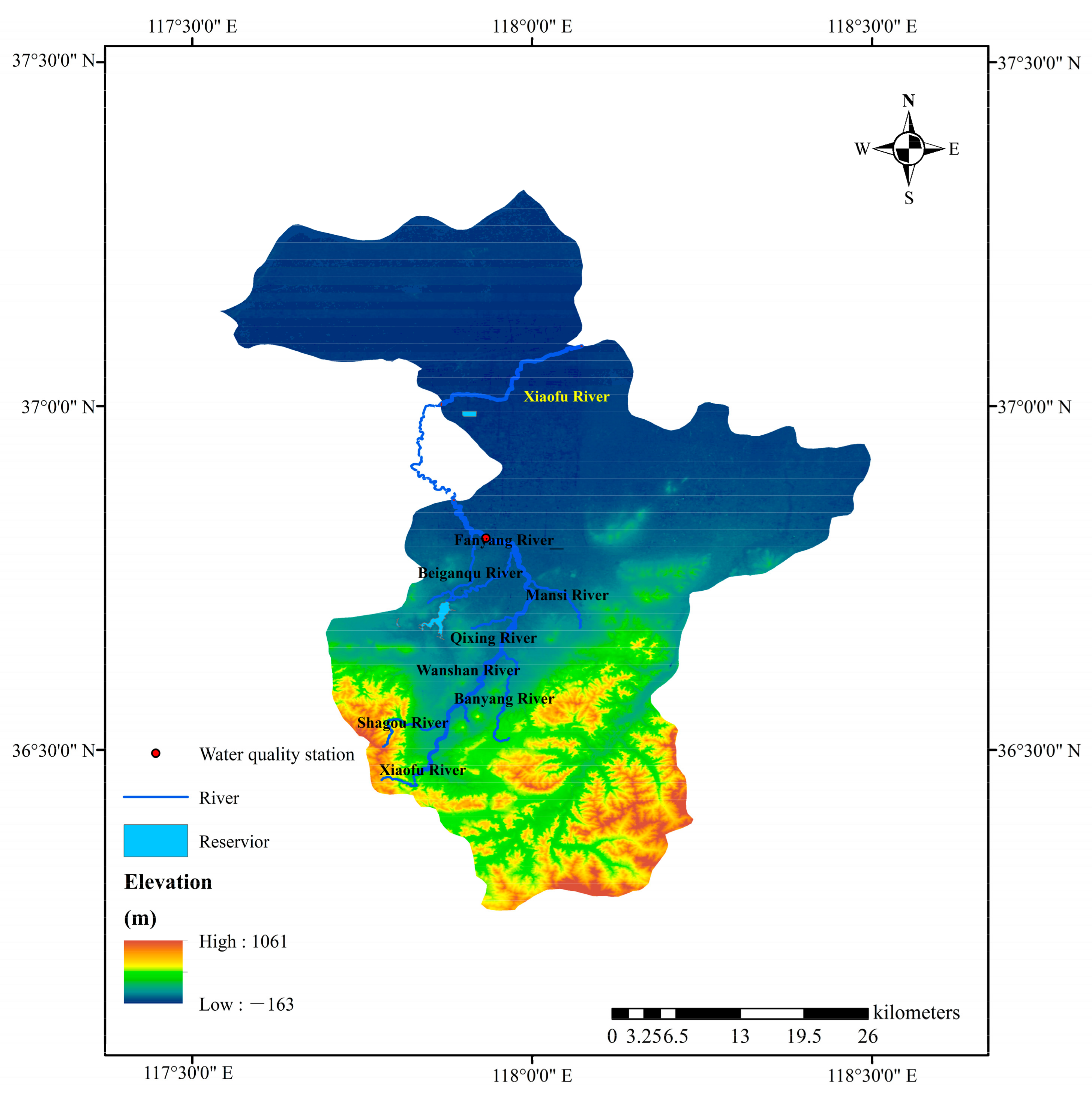
2.1. Study Area

The study area selected for this research is part of the Xiaofu River in Shandong Province, China (Figure 1). The study area is a temperate monsoon climate zone, with the same period of rain and heat, strong seasonal rainfall, and approximately 70% of annual precipitation falls during the flood season (June to September). The Xiaofu River is a first-class tributary on the right bank of the Xiaoqing River [35]. The total length of the river is 136 km. The average gradient of the river is 1.8/1000. The Xiaofu River basin is located at 36°25′N~37°07′ N, 117°42′E~118°08′ E. The watershed is 40 km wide from east to west and 76 km long from north to south, and the watershed area is 1705 km². The main tributaries are the Fanyang River, Banyang River, Mansi River, Gan River, Zhulong West River and others [36].

Since the 1980s, the Xiaofu River has been used as a sewage channel for factories, mines, enterprises, and residents along the river. In addition, rainfall is relatively low, so the water pollution of the Xiaofu River is significant [37]. The lack of water resources upstream of the Xiaofu River and the impact of sluice gates and dam impoundments have led to poor water connectivity, poor self-purification ability, and fragile aquatic ecosystems. In recent years, a series of water environment improvement projects have been carried out in the Xiaofu River basin, and the quality of water resources has improved, but the overall situation of the water environment is still not satisfactory. Predicting the water quality of the Xiaofu River can help design water environmental treatment plans.

2.2. Data Sources

In this paper, water quality data from the Zhangzhouluqiao Provincial Control Station along the Xiaofu River (36°48′19″ N, 117°56′08″ E) are used as the research object. The quality of the water collected from this station is poor, and there is great room for improvement. The main water quality indicators monitored are based on the Environmental Quality Standards for Surface Water (GB3838-2002) and include chemical oxygen demand (COD), ammonia nitrogen (NH₃-N), permanganate index (COD_Mn), pH, dissolved oxygen (DO), electrical conductivity, turbidity, and water temperature. The data were collected every 24 h from 13 April 2019, to 12 April 2021. There are a total of 1096 groups of data, which fully reflect the periodic changes in water quality. According to the water quality of the Xiaofu River, pH, DO, COD_Mn and NH₃-N were selected in this paper as the water quality prediction indicators. Statistical analysis was performed on the data series to check for missing data. The statistical analysis results are shown in

Table 1. Statistical descriptions of data series.

Variable Name	Description	Average	Standard Deviation	Maximum Value	Minimum Value	Number of Missing Data
pH	Pondus hydrogenii	7.912	0.437	8.83	6.02	0
DO	Dissolved oxygen (mg/L)	8.779	2.379	18.9	0.5	0
CODMn	Permanganate index (mg/L)	4.327	1.149	9	1.82	1
NH3-N	Ammonia nitrogen (mg/L)	0.472	0.415	5.16	0.028	1

, including average value, standard deviation value, maximum value, minimum value, and number of missing data. The values of water quality parameters meet the general water quality standards. The discrete degree of the pH and NH₃-N time series is small. The numbers of missing data in the water quality time series are very few.

3. Method

The prediction accuracy of LSTM for multiperiod hybrid water quality time series is not high. To improve the accuracy of LSTM in predicting water quality, a surface water quality prediction model based on EEMD–LSTM is developed. The flowchart for the EEMD–LSTM prediction model is shown in Figure 2.

The EEMD–LSTM consists of the following steps.

Step 1: Data preprocessing. The min-max normalization (MMN) method is used to normalize the original water quality series [38]. MMN can accelerate the speed of the gradient descent method to find the optimal solution and improve the accuracy of the prediction model. Then, the isolation forest algorithm is used to identify abnormal fluctuations, and the input and output samples are determined according to the selected sliding time window width.

Step 2: Series decomposition. After the preprocessing of the original water quality time series, EEMD is used to decompose the series into multiple components that contain high-frequency and low-frequency components. The high-frequency components mainly reflect the influence of sudden pollution and discontinuous nonpoint source pollution, and the low-frequency components mainly reflect the physicochemical properties and long-term trend of surface water quality.

Step 3: Period calculation. The fast Fourier transform (FFT) method can reflect the periodic characteristics of signals that cannot be extracted in the time domain from the frequency domain and is a commonly used signal analysis method [39]. The components that have a great impact on water quality changes are identified according to the significant period.

Step 4: Independent LSTM submodels are then developed for each decomposed component. When training the LSTM submodels, the mean squared error (MSE) of the training dataset is chosen as a criterion to calibrate the model, and the Adam algorithm is chosen as the optimizer. Finally, the prediction results of each submodel are aggregated to obtain the final water quality prediction results.

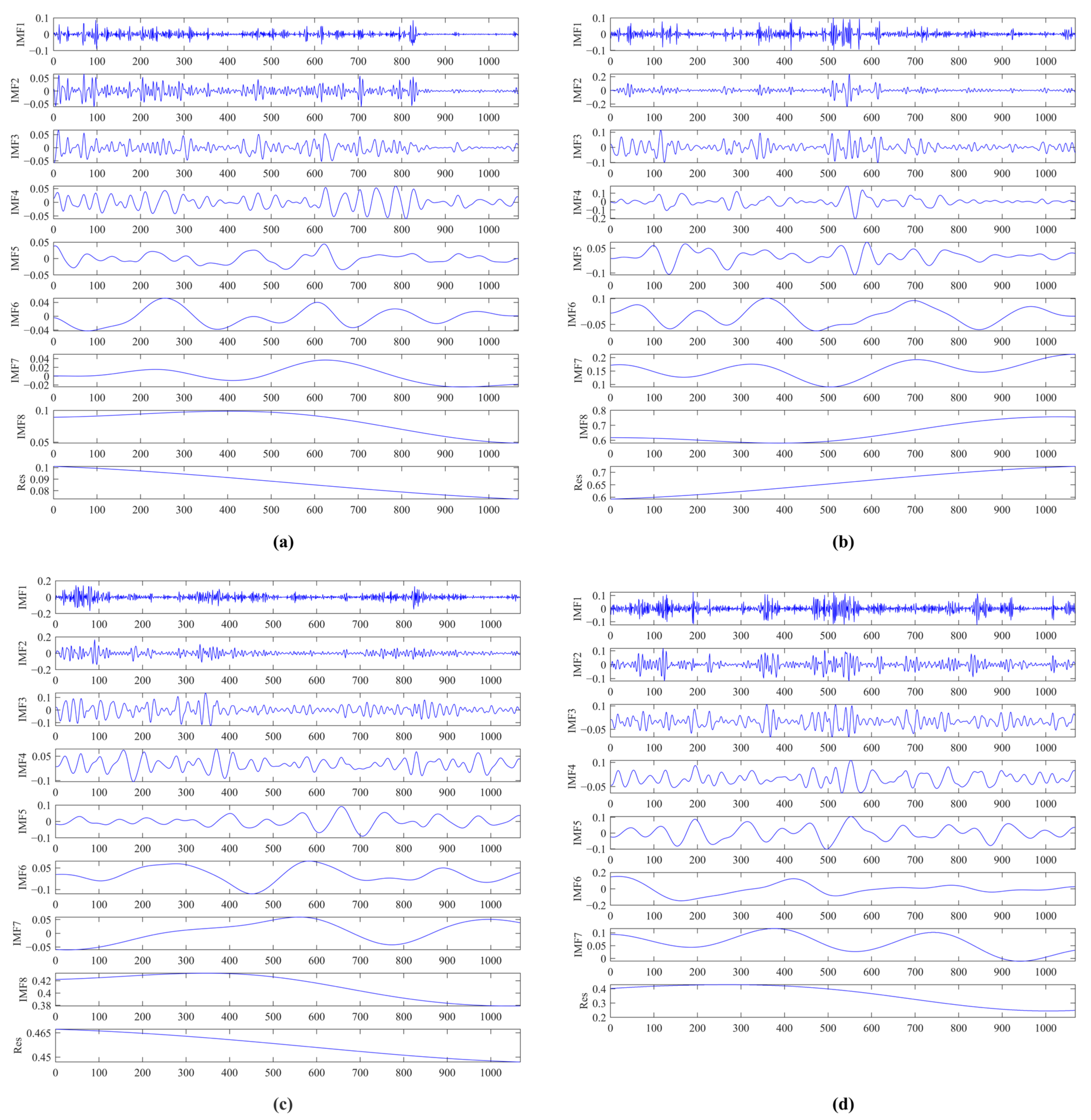
3.1. Ensemble Empirical Mode Decomposition (EEMD)

Huang et al. [30] proposed a new analysis and preprocessing method for nonlinear signals, which is referred to as empirical mode decomposition. This method is suitable for dealing with nonlinear and nonstationary time series. The EMD must obey the following two rules at the same time: (1) all the extrema and zero crossing numbers must be the same or different at most by one; (2) all upper and lower envelopes must be locally symmetrical along the time axis.

To solve the problem of mode mixing (i.e., decomposed IMFs that contain multiple frequencies), Zhaohua and Norden [31] proposed an ensemble empirical mode decomposition method. EEMD utilizes the sensitivity of the signal-to-noise, first adding Gaussian white noise to the original signal to match the signals of different frequencies to the corresponding time scale and then implementing the EMD process.

Given an original signal $x\left(t\right)$, the specific process of EEMD is as follows:

(1) Add Gaussian white noise to the original signal, $n^i\left(t\right)~N(0,{\sigma }^2)$.

$$x^i\left(t\right)=x\left(t\right)-n^i\left(t\right)$$

(1)

where $i$ represents the number of times Gaussian white noise is added.

(2) Decompose the mixed signal $x^i\left(t\right)$ by EMD into IMFs $C_j^i\left(t\right)$, ($j$ = 1, 2,…, n) and residual $r^i\left(t\right)$.

$$x^i\left(t\right)={\sum }_{j=1}^n{C}_j^i\left(t\right)+r^i\left(t\right)$$

(2)

where $C_j^i\left(t\right)$ represents the $j$th IMF component obtained by decomposing the $i$th mixed signal.

(3) Repeat the above steps $N$ times with different Gaussian white noise each time and find the corresponding IMFs.

(4) Average the summation of corresponding decomposed IMFs $N$ times to eliminate the influence of the added white noise on the original signal.

$$\stackrel{-}{C_j\left(t\right)}=\frac{1}{N}{\sum }_{j=1}^n{C}_j^i\left(t\right)$$

(3)

where $C_j^i\left(t\right)$ represents the $j$th IMF component.

Finally, after being decomposed by EEMD, the original signal $x\left(t\right)$ can be expressed as:

$$x\left(t\right)={\sum }_{j=1}^N\stackrel{-}{c_j\left(t\right)}+r\left(t\right),i=\mathrm{1,2},\dots ,N$$

(4)

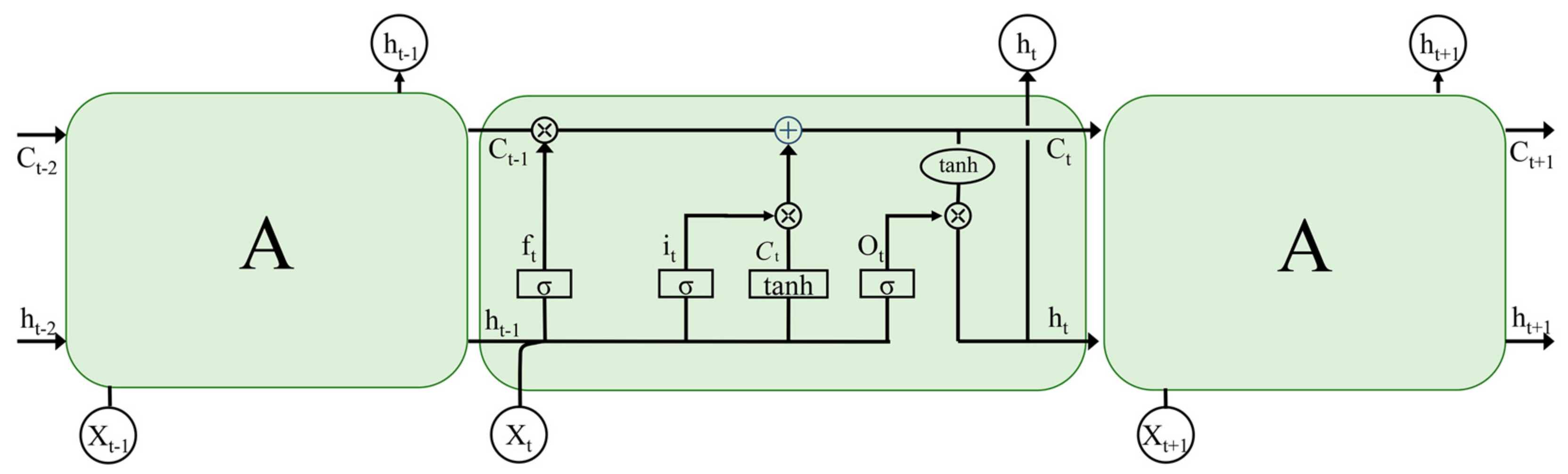
3.2. Long Short-Term Memory (LSTM)

A long short-term memory network is an improved network structure proposed on the basis of RNNs that effectively overcomes the long-term dependence problem and gradient vanishing problem of RNNs [24]. LSTM is suitable for processing and predicting events with long time intervals and delays in time series [23]. LSTM introduces gates, which can selectively remove or add information. The LSTM cell mainly includes four gate structures: forget gate, input gate, update gate and output gate [24]. The function of the forget gate is to forget the irrelevant state information of the previous moment. The input gate determines what information can enter the memory cell at the current moment. The output gate determines the output of the complex network. The memory unit of LSTM can use these three gate structures to screen long-term and short-term memory information. The general architecture of the LSTM cell is shown in Figure 3.

The key to LSTM is the transmission of the cell state, which controls the information passed into the network through the combination of three gates and determines the cell state. In Figure 3, $X_t$ represents the input of the network at time $t$, $h_t$ represents the output of the network at time $t$, and $C_t$ represents the cell state at time $t$.

$$f_t=\sigma (W_f*\left[h_{t-1},X_t\right]+b_f)$$

(5)

The operation ‘*’ represents the elementwise multiplication of the vectors.

$$i_t=\sigma (W_i*\left[h_{t-1},X_t\right]+b_i)$$

(6)

$$o_t=\sigma (W_o*\left[h_{t-1},X_t\right]+b_o)$$

(7)

$$\widetilde{C_t}=\mathrm{t}\mathrm{a}\mathrm{n}\mathrm{h}(W_c*\left[h_{t-1},X_t\right]+b_c)$$

(8)

$$C_t=f_t*C_{t-1}+i_t*\widetilde{C_t}$$

(9)

where $\sigma$ is the logistic sigmoid function ($\sigma \left(x\right)=\frac{1}{1+e^{-x}}$), $W_f$, $W_i$, $W_o$ and $W_c$ represent the weight matrices of the forget gate, the input gate, the output gate and the tanh layer, respectively, $b_f$, $b_i$, $b_o$ and $b_c$ represent the bias vectors of the forget gate, the input gate, the output gate and the tanh layer ($\tanh \left(x\right)=\frac{1-e^{-2x}}{1+e^{-x}}$), respectively, $f_t$, $i_t$ and $o_t$ represent the output of the forget gate, the input gate and the output gate at time $t$, respectively, and $\widetilde{C_t}$ is an update vector for the cell state.

Finally, the output $h_t$ of the memory cell is obtained through the hyperbolic tangent activation function tanh.

$$h_t=O_t* \mathrm{t}\mathrm{a}\mathrm{n}\mathrm{h} \left(C_t\right)$$

(10)

LSTM is suitable for processing and predicting time series data due to its good ability to deal with the long-term dependence problem on time series data and the problem of gradient disappearance.

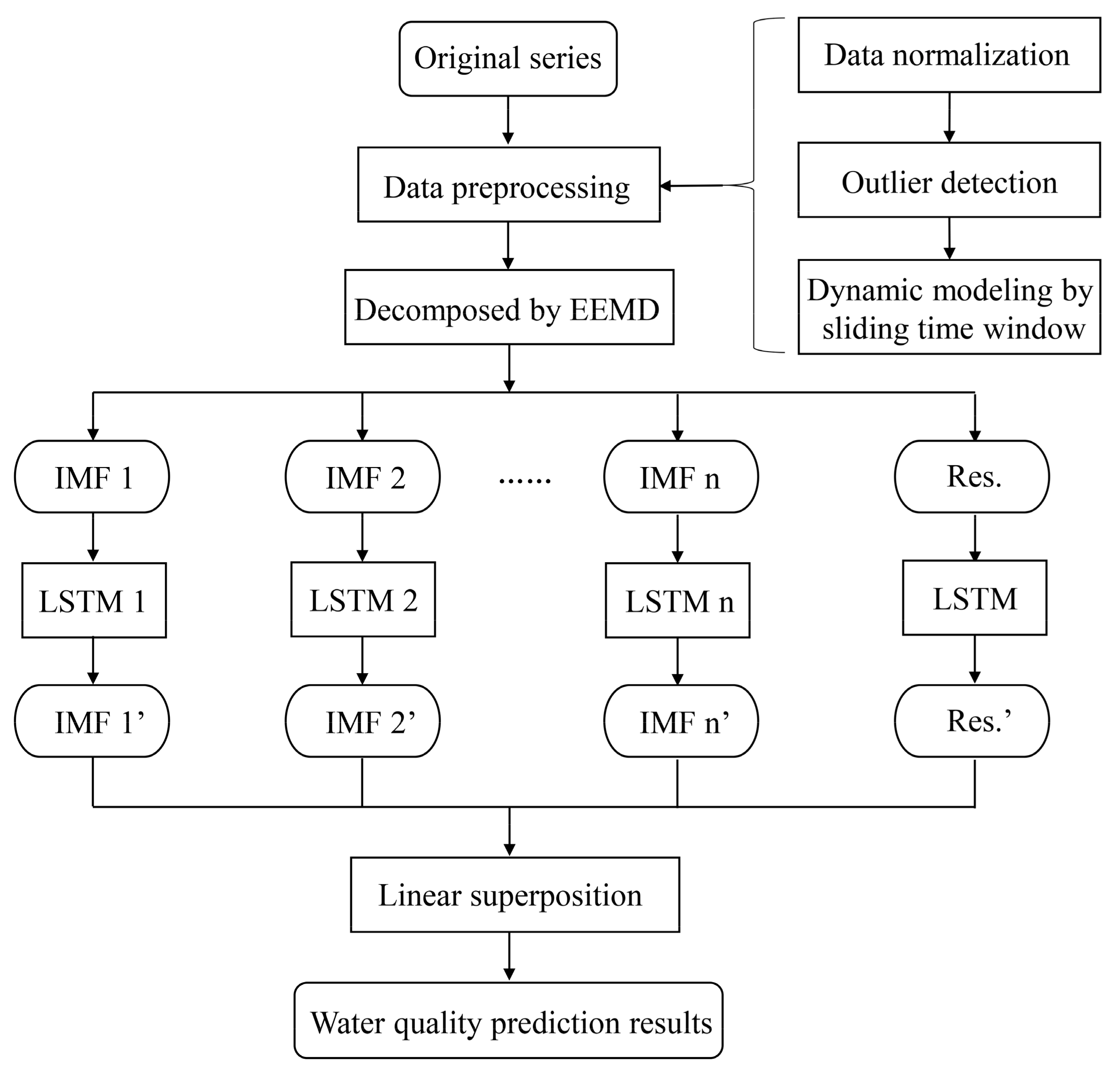
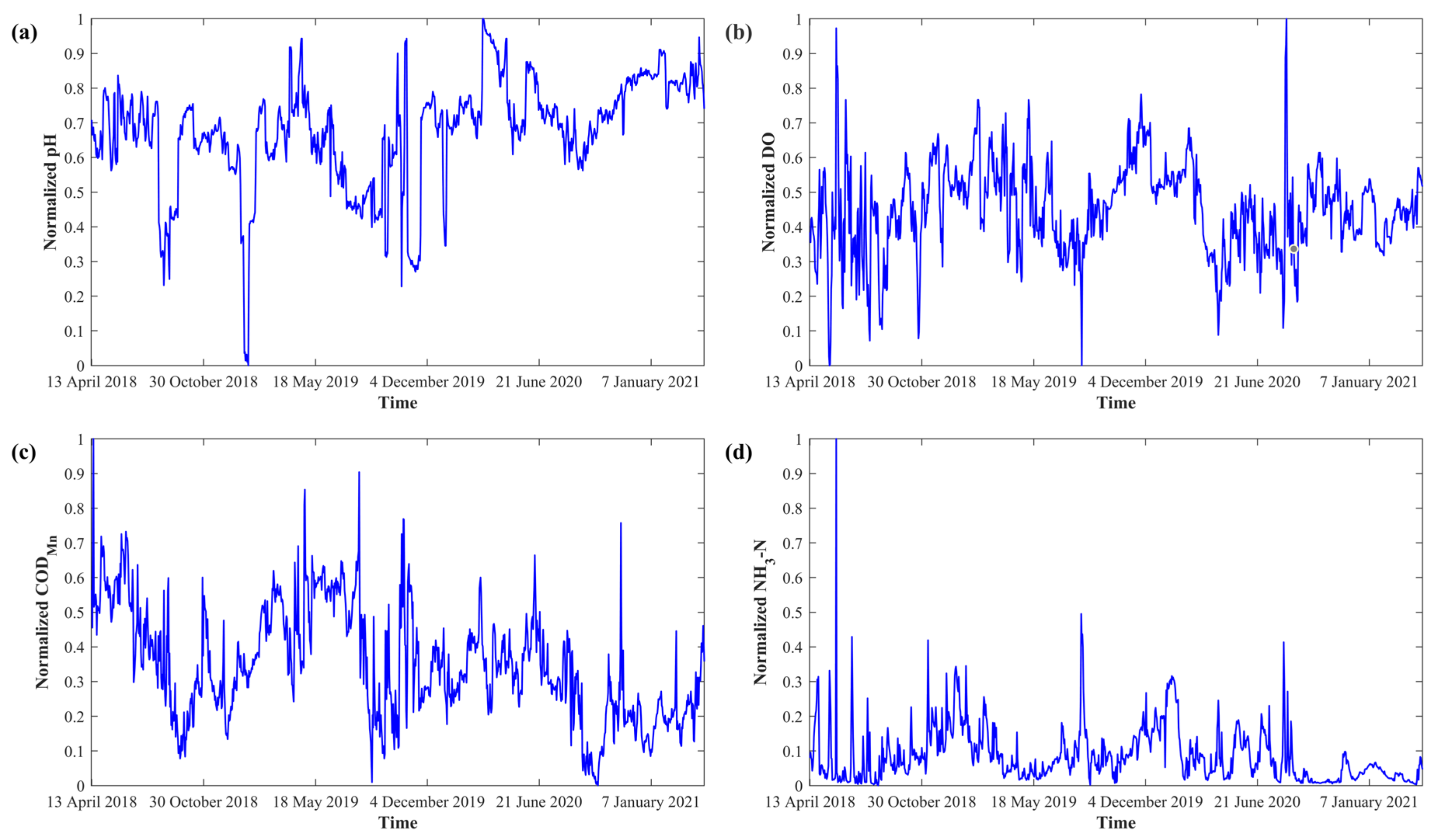
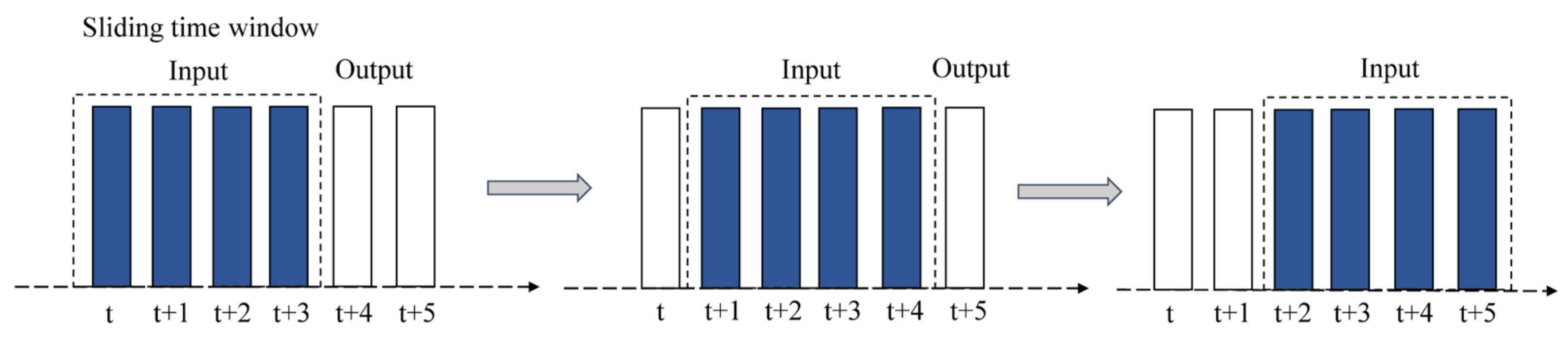
3.3. Data Preprocessing

3.3.1. Data Normalization

Data normalization is an important data preprocessing step that can accelerate the speed of the gradient descent method to find the optimal solution and improve the accuracy of the forecasting model. A large amount of unscaled data will slow the learning speed of the artificial neural network and the convergence speed of the model. Since LSTM is very sensitive to fluctuations in time series data and to capturing the trends in time series data, the data need to be normalized before being fed to the neural network [40]. Original data are normalized using the min-max normalization (MMN) method, which linearly scales unnormalized data to predefined lower and upper bounds [38]. The equation is given as follows:

$$x_n=\frac{x-x_{min}}{x_{max}-x_{min}}$$

(11)

where $x_n$ represents the normalized time series data, $x$ represents the original time series data, $x_{min}$ represents the minimum value of the time series data, and $x_{max}$ represents the maximum value of the time series data. The min-max normalization method scales the data between 0 and 1.

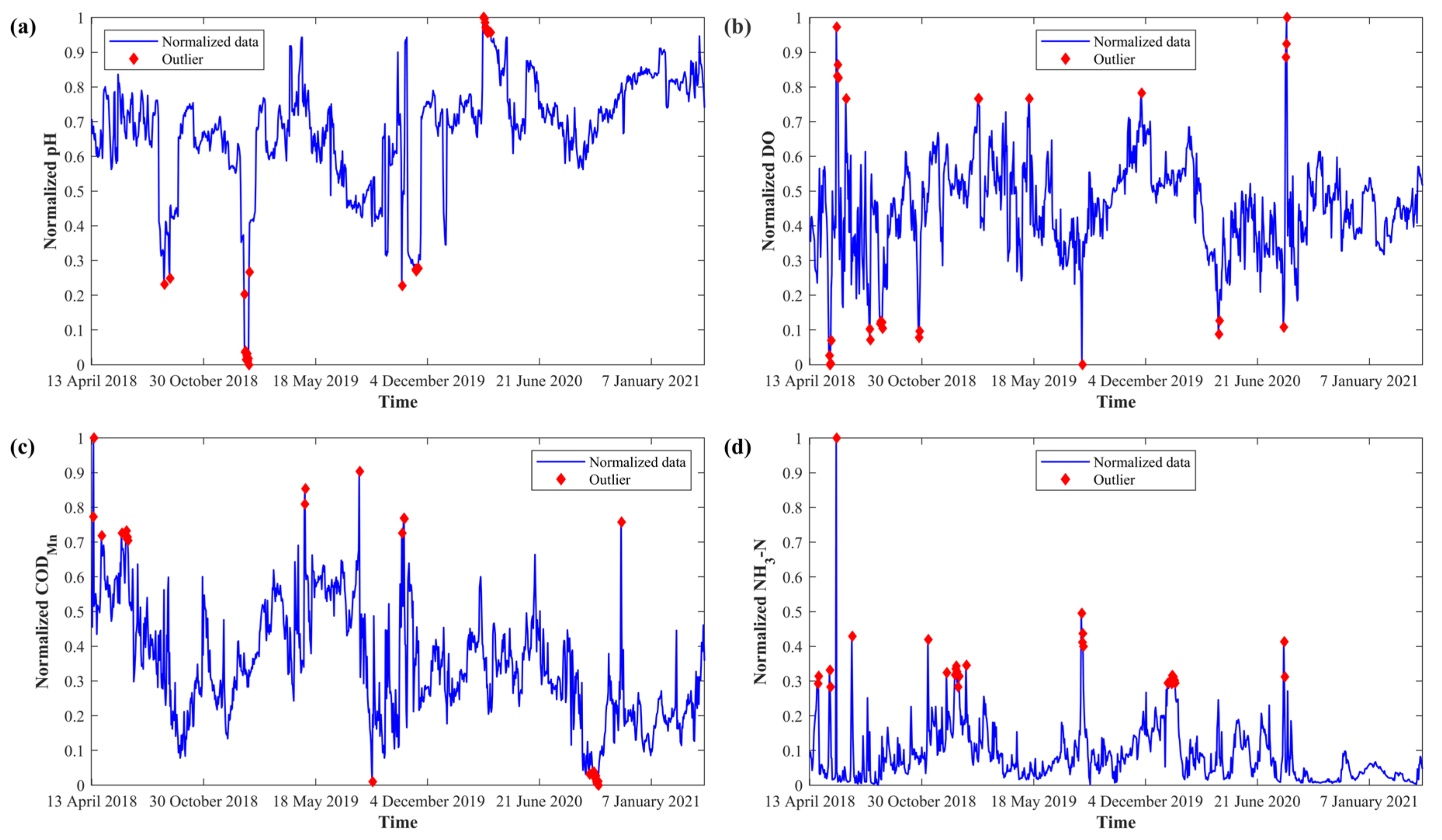
3.3.2. Outlier Detection

The real-time monitoring data of water quality are usually unprocessed raw data. Weather factors, such as strong wind and heavy rainfall, may affect the results of real-time water quality monitoring, and problems, such as abnormal monitoring equipment or manual input errors, will lead to missing values, abnormal values or noise in the original data. Abnormal values will affect the accuracy of the model prediction. Certain methods are used to identify these outliers and deal with them. The characteristics of abnormal data are as follows: (1) they represent a small proportion of the sample data; and (2) they have significantly different properties compared with normal sample data.

Liu et al. [41] proposed the isolation forest algorithm and applied it to data outlier detection. The isolation forest algorithm has a linear time complexity and high accuracy and is a neural network algorithm that meets the requirements of big data processing. Any outlier detection method requires an anomaly score, and the calculation equation of the search path length of the isolation forest is as follows:

$$c\left(n\right)=2H\left(n-1\right)-\left(\frac{2\left(n-1\right)}{n}\right)$$

(12)

where $n$ is the number of samples, $H\left(i\right)$ is the harmonic number and can be estimated by $ln\left(i\right)+\xi$ (Euler’s constant), and $c\left(n\right)$ is the average path length of the binary search tree.

By normalizing the length of the isolated binary tree, a number between 0 and 1 can be obtained as the abnormal score of the detected sample. The anomaly score $s$ of an instance $x$ is defined as:

$$s(x,n)=2^{\frac{E\left(h\left(x\right)\right)}{c\left(n\right)}}$$

(13)

where $h\left(x\right)$ represents the path length from the root node to the $x$ node, and $E\left(h\right(x\left)\right)$ is the average of the path lengths of all the isolated trees in the isolated forest for the sample point $x$. When the anomaly score is larger, the sample point is more likely to be an outlier. Based on the anomaly score $s$, we can make the following assessments [41]:

(1)

If the anomaly score is very close to 1, then the data are definitely anomalies.

(2)

If the anomaly score is much smaller than 0.5, then it is safe to regard the data as normal instances.

(3)

If all the anomaly scores are approximately 0.5, then there are no distinct outliers in the sample.

3.4. Performance Evaluation

To objectively and comprehensively evaluate the prediction performance of each model, four different evaluation indicators are selected: root mean square error (RMSE), mean absolute error (MAE), mean absolute percentage error (MAPE) and determination coefficient (R²). RMSE is sensitive to errors that are evident in the experimental data. MAE is the average value of absolute error and can truly reflect the state of the model’s error in prediction. MAPE is the expected value of the absolute error and percentage of the true value. The values of RMSE, MAE, and MAPE are all from 0 to +∞. The smaller the RMSE, MAE, and MAEP, the more accurate the prediction result and the better the model effect. The value of the determination coefficient R² is between 0 and 1, and the closer to 1 the value is, the better the model’s prediction ability of the regression effect. Generally, if the coefficient of determination exceeds 0.8, the model is considered to have high goodness of fit. The specific calculation equation of each loss function is as follows:

$$\mathrm{R}\mathrm{M}\mathrm{S}\mathrm{E}=\sqrt{\frac{1}{N}\sum _{i=1}^N{(y_i-y_i^{*})}^2}$$

(14)

$$\mathrm{M}\mathrm{A}\mathrm{E}=\frac{1}{N}\sum _{i=1}^N{|y}_i-y_i^{*}|$$

(15)

$$\mathrm{M}\mathrm{A}\mathrm{P}\mathrm{E}=\frac{1}{N}\sum _{i=1}^N\left|\frac{y_i-y_i^{*}}{y_i}\right|\times 100\%$$

(16)

$${\mathrm{R}}^2=1-\frac{{\sum }_{i=1}^N{(y_i-y_i^{*})}^2}{{\sum }_{i=1}^N{(y_i-\stackrel{-}{y_i})}^2}$$

(17)

where $N$ is the number of samples, $y_i$ is the measured value, $y_i^{*}$ is the predicted value, and $\stackrel{-}{y_i}$ is the average value of the measured data.

The values of RMSE, MSE, and MAPE are not of the same order of magnitude for different water quality parameters. Therefore, we primarily use R² as the main criterion for model selection, with higher values indicating better prediction ability. Additionally, considering other performance evaluators, such as RMSE, MAE, and MAPE, can provide a more comprehensive evaluation of the model’s accuracy and prediction performance.

4. Results

4.1. Data Preprocessing

Since there were few missing data (<10%) in the water quality time series, the mean smoothing method was used to fill in the missing part of the data; the missing data were replaced by the average value of the two adjacent data on the left and right of the missing data. The min-max normalization method was used to convert the original values into values between [0, 1]. The normalization results are shown in Figure 4. This figure shows that the water quality parameters have apparent fluctuations.

The isolated forest algorithm described above was used to identify abnormal fluctuations, such as some data jumps in the original series of water quality parameters (the maximum abnormal sample ratio was set to 0.025), and the outliers were marked. The outlier identification results are shown in Figure 5. Considering the small number of outliers and the large difference between an outlier and its adjacent values, outliers were directly removed from the original series, and the average value of the data on both sides of an outlier was used to fill missing values. This figure shows that compared with the original series, obvious outliers in the denoised water quality time series were removed. However, this time series is still complex and has obvious nonstationary and nonlinear characteristics from the overall trend. Measures are still needed to reduce the complexity of the water quality time series.

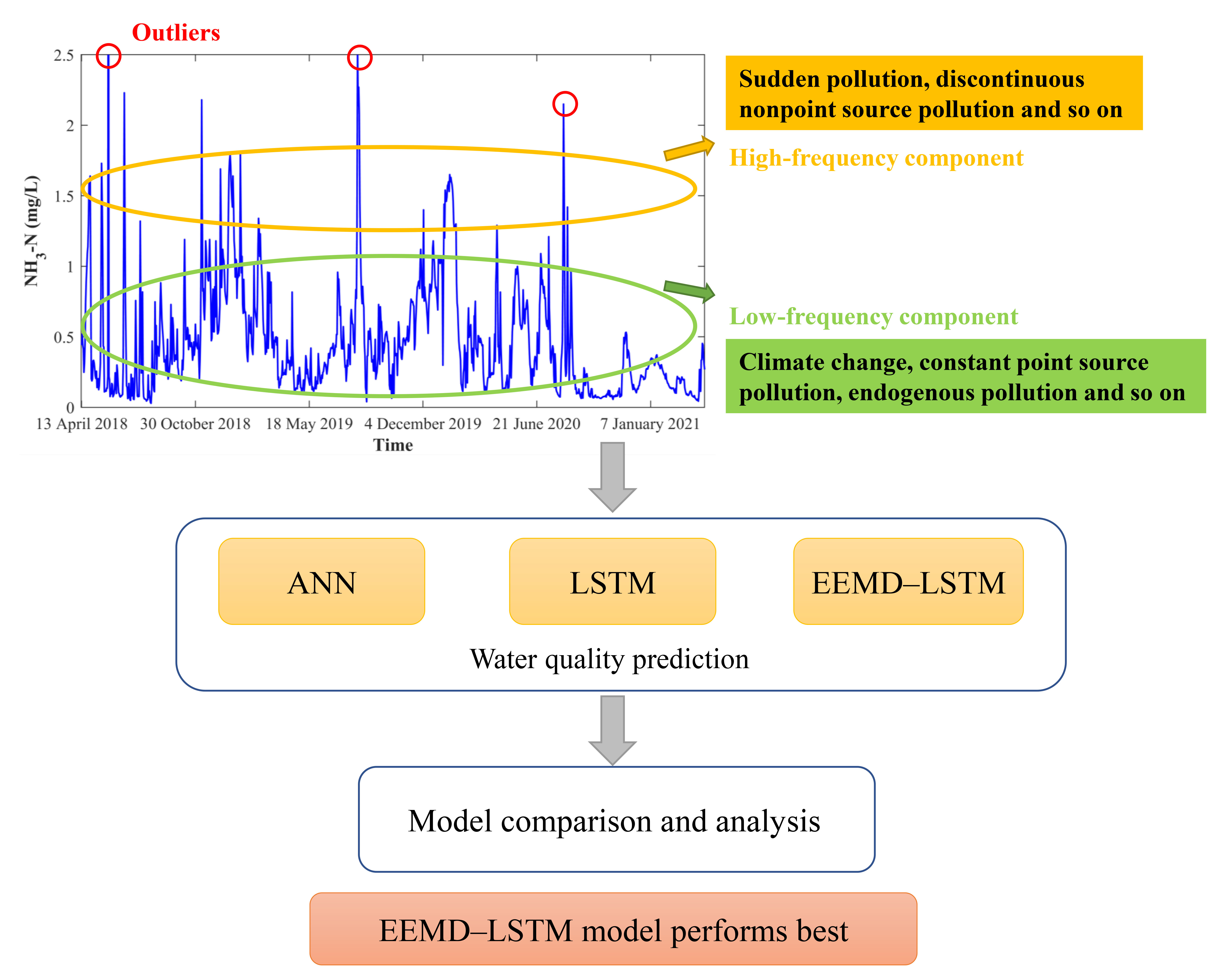
4.2. EEMD Decomposition Results

After data preprocessing, the water quality time series was decomposed by the EEMD method. The ensemble number was set to 100, and the standard deviation of Gaussian white noise $n^i\left(t\right)$ was 0.05 [42,43]. The EEMD results of each water quality parameter are shown in Figure 6. The NH₃-N, pH and DO time series were decomposed into eight IMFs and one residual item Res and arranged in the order of frequency from high to low. The COD_Mn time series was decomposed into seven IMFs and one residual item Res.

The first four IMF components fluctuate greatly, among which IMF1 has the strongest nonlinearity, the largest amplitude and the highest frequency. The residual item can represent the long-term trend of the time series [42,43]. As illustrated in Figure 6, the residual items of the NH₃-N and COD_Mn time series have obvious declining trends, indicating that the water environmental control measures of the Xiaofu River achieved some results in recent years.

In this paper, the FFT method was used to find the significant period of each IMF component, and the period with the largest autocorrelation coefficient was used as the period of the time series. The residual item (Res) represents the long-term trend of the water quality time series, so Res is not calculated in the period extraction of each IMF component in the following. The period identification results of IMF components for different water quality parameters are shown in

Table 2. The period of IMF components for water quality parameters.

Variable Name	Period (Day)
	IMF1	IMF2	IMF3	IMF4	IMF5	IMF6	IMF7	IMF8
NH3-N	3	7	38	41	152	356	534	534
pH	3	7	22	53	89	356	534	534
DO	5	9	20	42	97	356	356	534
CODMn	4	8	12	59	66	356	356	-

.

Table 2 shows that the period of the first two IMF components is 3–9 days, which corresponds to the number of days that the pollutants are naturally degraded in the water body. Therefore, IMF1 and IMF2 may represent the fluctuation of water quality due to water affected by sudden pollution, discontinuous nonpoint source pollution and so on. IMF3–IMF5 mainly reflect the seasonal changes in water quality, and IMF6–IMF8 mainly reflect the interannual changes in water quality. The seasonal and interannual changes in the water quality series are relatively stable, but the fluctuations caused by sudden pollution and discontinuous nonpoint source pollution are large and complex. Therefore, to obtain more accurate water quality prediction results, it is necessary to accurately simulate the high-frequency components. The EEMD method is able to separate the high-frequency components, enhance the details and transform nonlinear water quality series into several relatively simple and stationary time series that help improve prediction results.

4.3. Model Training and Parameter Optimization

In this paper, we chose the MSE of the training dataset as a criterion to calibrate the model and chose the Adam algorithm as the optimizer. The Adam algorithm can solve the problems of a disappearing learning rate and slow convergence property of the error term. It can optimize the performance of the model and has lower running costs with high computational efficiency and less running memory [44]. The Adam algorithm was adopted to train the model multiple times and update the parameters continuously. When the error between the actual value and the predicted value meets the accuracy requirements, the model was saved. The hyperparameters of the LSTM model were finally determined, as shown in

Table 3. The optimal parameters and structure of LSTM.

Parameter Name	Number
epochs	100
batch size	16
number of LSTM layers	1
number of neurons in the input layer	1
number of neurons in the hidden layer	50
number of neurons in the output layer	1

. The number of neurons was 50, the number of epochs for each training was 100, and the batch size was 16. In general, the larger the batch size, the faster the training. However, if the batch size is too large, the network easily converges to the local optimum [45].

Different sliding time window widths n impact the output of the model. In this paper, the water quality time series of the corresponding time width was divided from the dataset as the input sample, and one time step water quality value after the sliding window was used as the output sample. Using n = 4 as an example, its dynamic modeling process is shown in Figure 7.

To improve the prediction accuracy of the model, the model performance is compared under different sliding time window widths, and the results are shown in

Table 4. The LSTM model performance under different sliding time window widths.

Water Quality Indicator	Sliding Time Window Width	RMSE (mg/L)	MAE (mg/L)	MAPE (%)	R2
NH3-N	4	0.096	0.071	67.387	0.423
	5	0.089	0.057	31.901	0.783
	6	0.089	0.060	42.082	0.727
	7	0.089	0.059	39.477	0.746
	8	0.093	0.067	60.726	0.545
pH	4	0.080	0.049	1.787	0.656
	5	0.078	0.045	1.425	0.741
	6	0.078	0.046	1.521	0.722
	7	0.078	0.046	1.558	0.721
	8	0.087	0.059	1.908	0.656
DO	4	0.590	0.420	7.831	0.769
	5	0.587	0.424	7.600	0.772
	6	0.594	0.434	7.741	0.763
	7	0.591	0.429	7.630	0.769
	8	0.588	0.422	7.628	0.777
CODMn	4	0.246	0.167	11.041	0.748
	5	0.247	0.168	12.646	0.724
	6	0.244	0.165	11.538	0.743
	7	0.249	0.170	10.615	0.752
	8	0.243	0.165	11.701	0.744

. This result illustrates that the optimal sliding time window widths for NH₃-N, pH, DO and COD_Mn are 5, 5, 8 and 7, respectively.

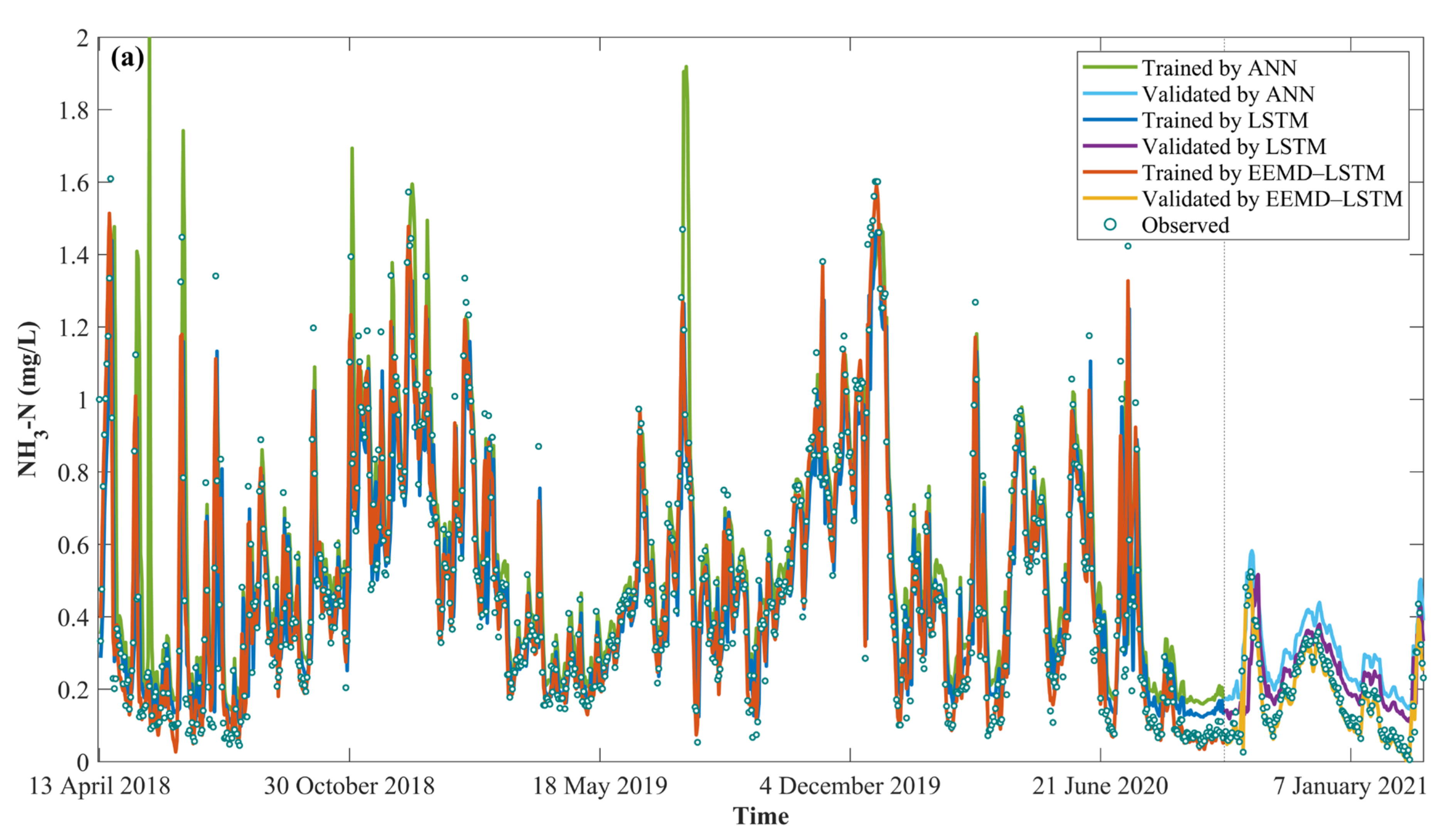
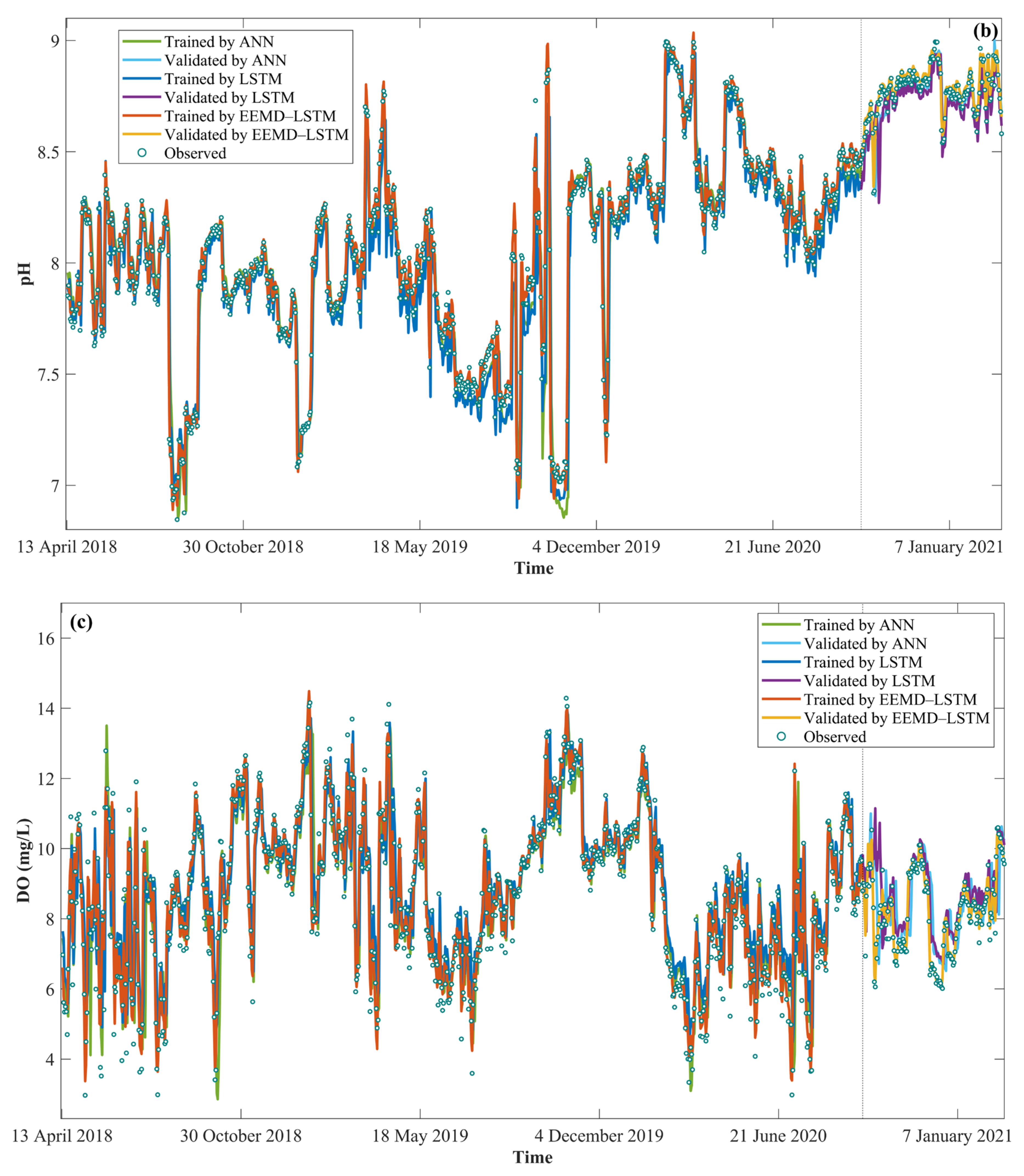
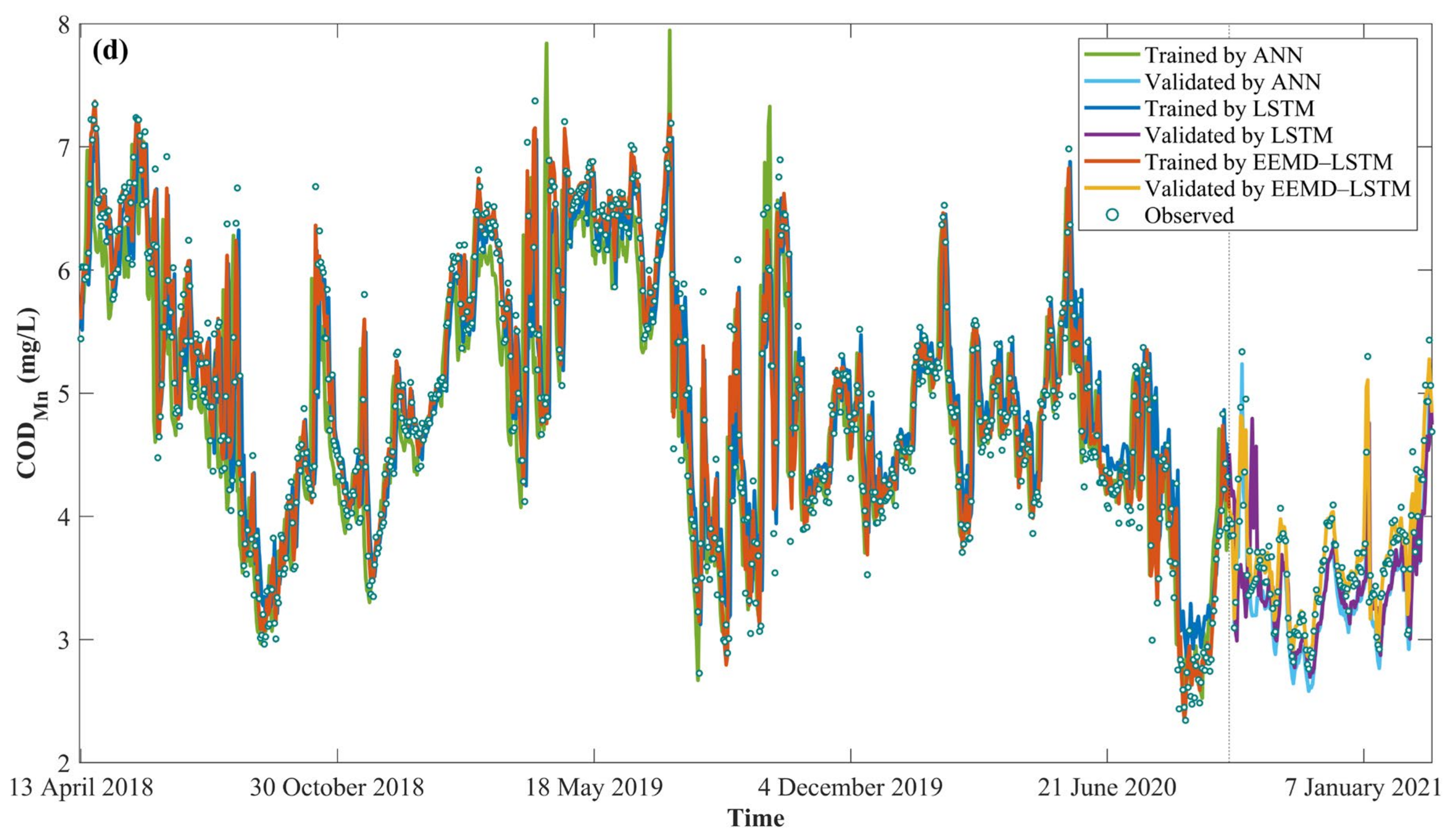
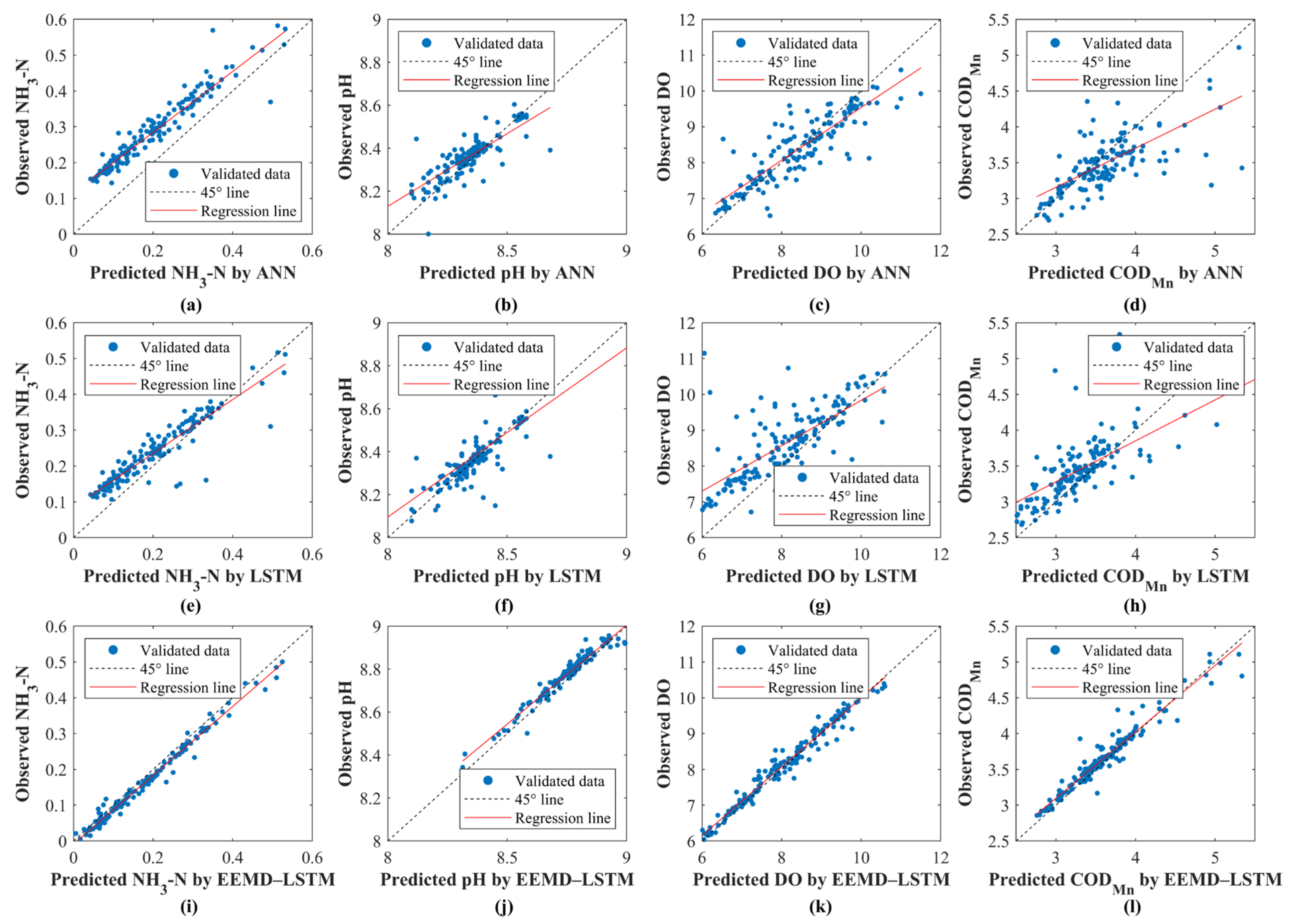
4.4. Water Quality Prediction by EEMD–LSTM

The water quality data were divided into a training period and validation period; the first 85% of the data were from the training period, and the last 15% of the data were from the validation period. After the model is trained, the learning situation of the model can be judged by the loss curve. If the loss curve declines smoothly or continues to decline at the end of the training period, it indicates that there is an underfitting phenomenon. If the loss curve continues to decline, but begins to rise at a certain point or there is an upward trend in the fluctuation, it means that there is an overfitting phenomenon. When the loss values of the model in the training period and the validation period decrease and become stable at the same time, the model training effect is good and can be used for water quality prediction.

To fully verify the performance of EEMD–LSTM, ANN, LSTM, and EEMD–LSTM were used to predict water quality parameters using the same data as input. The prediction results of ANN, LSTM, and EEMD–LSTM are shown in Figure 8, and their performance metrics results are listed in

Table 5. Model performance comparison of ANN, LSTM, and EEMD–LSTM.

Model	Water Quality Indicator	Training				Validation
		RMSE (mg/L)	MAE (mg/L)	MAPE (%)	R2	RMSE (mg/L)	MAE (mg/L)	MAPE (%)	R2
ANN	NH3-N	0.268	0.148	51.028	0.615	0.018	0.017	89.344	0.315
	pH	0.167	0.107	1.393	0.851	0.026	0.017	2.106	0.627
	DO	1.311	0.889	13.245	0.713	0.031	0.022	5.022	0.757
	CODMn	0.587	0.426	8.835	0.703	0.062	0.039	19.208	0.462
LSTM	NH3-N	0.169	0.111	37.694	0.754	0.110	0.109	50.381	0.567
	pH	0.136	0.080	1.032	0.872	0.122	0.113	1.554	0.657
	DO	1.151	0.826	10.807	0.733	1.027	0.820	4.685	0.817
	CODMn	0.457	0.314	7.239	0.811	0.440	0.326	13.990	0.693
EEMD–LSTM	NH3-N	0.077	0.050	5.419	0.950	0.022	0.019	3.150	0.924
	pH	0.047	0.032	0.321	0.988	0.035	0.029	0.273	0.965
	DO	0.531	0.355	2.245	0.945	0.224	0.161	0.994	0.961
	CODMn	0.189	0.131	2.756	0.969	0.133	0.085	2.219	0.936

. It can be seen from Figure 8 that the performance of LSTM and EEMD–LSTM is better than the performance of ANN in water quality prediction. Although LSTM can predict the trend of water quality changes, the error between observed and predicted values is large, and the prediction accuracy of details and jump points is insufficient. EEMD–LSTM can more accurately predict the detailed changes and greatly improve the model performance in terms of the hysteresis problem. It is also evident in Table 5 that the EEMD–LSTM model outperforms ANN and LSTM in water quality time series prediction. Compared with LSTM, the prediction accuracy of EEMD–LSTM on the four evaluation indicators of RMSE, MAE, MAPE and R² has improved. The RMSE, MAE, and MAPE of NH₃-N decreased by 80.0%, 82.6%, and 93.7%, respectively, and R² increased by 63.0%. The RMSE, MAE, and MAPE of pH decreased by 71.3%, 74.3%, and 82.4%, respectively, and R² increased by 46.9%. The RMSE, MAE, and MAPE of DO decreased by 78.2%, 80.4%, and 78.8%, respectively, and R² increased by 17.6%. The RMSE, MAE, and MAPE of COD_Mn decreased by 69.8%, 73.9%, and 84.1%, respectively, and R² increased by 35.1%. These indicators illustrate that the EEMD method can better extract essential features of the water quality time series and reduce the interference of random factors. They also indicate that the prediction performance of the model is greatly improved with the EEMD method. Figure 8 also shows that compared with the single LSTM model, the predicted values of EEMD–LSTM are closer to the observed values in the extreme value prediction.

A scatterplot of the observed and predicted values of the three models during the validation period is shown in Figure 9. The scatterplot intuitively shows that the EEMD–LSTM prediction results are closer to the observed value and have better performance.

In addition, the reason why EEMD–LSTM improves water quality prediction performance is further discussed. There are seasonal changes, interannual changes and short-term fluctuations in surface water quality parameters. The subsequences obtained by decomposing the original water quality sequence can more clearly show the seasonal periodic changes, interannual periodic changes and short-term fluctuations and reduce the complexity of the input data, which is beneficial to the learning and training of the model. At the same time, the high-frequency components IMF1 and IMF2 decomposed by the EEMD method can reflect the fluctuations in the water quality series caused by sudden pollution, and the prediction of these components separately can effectively improve the prediction accuracy.

5. Discussion

LSTM has achieved high accuracy prediction results in applications of many fields. However, the prediction accuracy of water quality is not satisfactory, as water quality series are generally multiperiod hybrid time series that have strong nonlinear and nonstationary characteristics, and LSTM is not suitable for predicting multiperiod hybrid time series. In this paper, we introduced the EEMD method to decompose the water quality time series into several simpler single-period components. The EEMD method can decompose the original water quality series into some components arranged from high frequency to low frequency. Among the IMFs decomposed by EEMD, IMF1 and IMF2 reflect the changing process of sudden pollutants discharged into surface water, and these components have great impacts on the accuracy of water quality prediction. The main difficulty in water quality prediction is accurately predicting the extreme water quality time series values. The extreme values are mainly affected by sudden pollution and dis-continuous nonpoint source pollution. We can focus on IMF1 and IMF2 to enhance the details and reduce the impact of interference information. Predicting these high-frequency components separately can improve the accuracy in predicting extreme values and the overall performance of the model. Therefore, the predicted values of EEMD–LSTM are closer to the observed values in the extreme value prediction, and the whole prediction accuracy of the EEMD–LSTM model is also improved compared with the single LSTM model.

The EEMD–LSTM model achieved good results in the time series prediction of water quality. The MAE, MAPE and RMSE of EEMD–LSTM for DO are 0.161, 0.994 and 0.224, respectively. The performance predictors of other water quality parameters also achieved high accuracy. Li et al. [46] developed a multimodal water quality prediction model called MSVR and proved that the combination of EEMD and SVR could achieve better prediction performance. The MAE, MAPE and RMSE of MSVR for DO were 0.175, 2.153 and 0.228, respectively [46]. This shows that EEMD–LSTM is reliable in predicting water quality. Limited by time and effort, only the performance of the hybrid model EEMD–LSTM was studied in this paper for water quality prediction. Subsequently, other methods to improve the performance of LSTM will be considered.

The influence of different sliding time window widths on the prediction accuracy is also discussed in this paper. The optimal sliding time window width of different water quality parameters is different, which is related to the migration, transformation and degradation rates of pollutants in water. The degradation coefficients of COD_Mn and NH₃-N in rivers are 0.08–0.15 and 0.2–0.44 day⁻¹, respectively [47]. Therefore, the residence times of COD_Mn and NH₃-N in water are 6.7–12.5 and 2.3–5 days. The optimal sliding time window widths for NH₃-N, pH, DO and COD_Mn are 5, 5, 8 and 7, respectively. This indicates that the optimal sliding time window width is consistent with the degradation time of pollutants in water. This is because after pollutants are discharged into the water, the concentration of pollutants at any point in the water increases with time and then tends to balance to the equilibrium value. As the number of predicted time steps increases, the prediction accuracy of the model will decline, so the EEMD–LSTM model can only predict short time steps at present. Water quality prediction over long time steps is still a challenging issue.

6. Conclusions

To achieve highly accurate water quality prediction results, a water quality prediction model based on the combination of the EEMD method and LSTM network is developed in this paper. The water quality monitoring data of the Xiaofu River are used as a sample for verification, and the four water quality parameters (NH₃-N, pH, DO, COD_Mn) of the Xiaofu River are predicted. The following conclusions were drawn from this study:

(1)

The EEMD method can decompose time series into components arranged from high frequency to low frequency. In this study, it is used to decompose the water quality time series to obtain several single-period components, which can effectively reduce the complexity and nonlinearity of the original time series. Among all components, the high-frequency components have the greatest impact on the accuracy of water quality prediction. Predicting the high-frequency components and the low-frequency components separately when using LSTM can significantly improve model accuracy.

(2)

Compared with LSTM, EEMD–LSTM significantly improves the accuracy of water quality prediction and greatly improves the model performance in terms of the hysteresis problem. During the validation period, the RMSE, MAE, MAPE and R² of EEMD–LSTM for NH₃-N were 0.022 mg/L, 0.019 mg/L, 3.150% and 0.924, respectively. The RMSE, MAE, MAPE and R² of EEMD-LSTM for pH were 0.035 mg/L, 0.029 mg/L, 0.273% and 0.965, respectively. The RMSE, MAE, MAPE and R² of EEMD-LSTM for DO were 0.224 mg/L, 0.161 mg/L, 0.994% and 0.961, respectively. The RMSE, MAE, MAPE and R² of the EEMD-LSTM for COD_Mn were 0.133 mg/L, 0.085 mg/L, 2.219% and 0.936, respectively. This shows that EEMD–LSTM has high prediction accuracy and strong generalization ability. In addition, the predicted values of EEMD–LSTM are closer to the observed values in the extreme value prediction.

In summary, EEMD–LSTM can be an effective tool for water quality prediction. The EEMD–LSTM model can quickly and accurately predict water quality changes, which can reflect the trend of future water quality changes and can provide a basis for formulating water environment governance measures. In future work, model structure optimization and other hybrid models can be tried. In addition, the spatial and temporal relationships between upstream and downstream are not considered in water quality prediction. This can be added to the developed algorithm in future work.

References

1. Tang, W.; Pei, Y.; Zheng, H.; Zhao, Y.; Shu, L.; Zhang, H. Twenty years of China's water pollution control: Experiences and challenges. Chemosphere 2022, 295, 133875. [Google Scholar] [CrossRef] [PubMed]
2. Xiong, Y.; Ran, Y.; Zhao, S.; Zhao, H.; Tian, Q. Remotely assessing and monitoring coastal and inland water quality in China: Progress, challenges and outlook. Crit. Rev. Environ. Sci. Technol. 2020, 50, 1266–1302. [Google Scholar] [CrossRef]
3. Liang, Z.; Zou, R.; Chen, X.; Ren, T.; Su, H.; Liu, Y. Simulate the forecast capacity of a complicated water quality model using the long short-term memory approach. J. Hydrol. 2022, 581, 124432. [Google Scholar] [CrossRef]
4. Yu, J.; Kim, J.; Li, X.; Jong, Y.; Kim, K.; Ryang, G. Water quality forecasting based on data decomposition, fuzzy clustering and deep learning neural network. Environ. Pollut. 2022, 303, 119136. [Google Scholar] [CrossRef]
5. Bui, H.H.; Ha, N.H.; Nguyen, T.N.D.; Nguyen, A.T.; Pham, T.T.H.; Kandasamy, J.; Tien, V.N. Integration of SWAT and QUAL2K for water quality modeling in a data scarce basin of Cau River basin in Vietnam. Ecohydrol. Hydrobiol. 2019, 19, 210–223. [Google Scholar] [CrossRef]
6. Bai, J.; Zhao, J.; Zhang, Z.; Tian, Z. Assessment and a review of research on surface water quality modeling. Ecol. Model. 2022, 466, 109888. [Google Scholar] [CrossRef]
7. Qin, Z.; He, Z.; Wu, G.; Tang, G.; Wang, Q. Developing Water-Quality Model for Jingpo Lake Based on EFDC. Water 2022, 14, 2596. [Google Scholar] [CrossRef]
8. Kang, M.; Tian, Y.; Zhang, H.; Wan, C. Effect of hydrodynamic conditions on the water quality in urban landscape water. Water Supply 2021, 22, 309–320. [Google Scholar] [CrossRef]
9. Samaneh, A.; Sedghi, H.; Hassonizadeh, H.; Babazadeh, H. Application of Water Quality Index and Water Quality Model QUAL2K for Evaluation of Pollutants in Dez River, Iran. Water Resour. 2021, 47, 892–903. [Google Scholar] [CrossRef]
10. Obin, N.; Tao, H.; Ge, F.; Liu, X. Research on Water Quality Simulation and Water Environmental Capacity in Lushui River Based on WASP Model. Water 2021, 13, 2819. [Google Scholar] [CrossRef]
11. Shabani, A.; Zhang, X.; Chu, X.; Zheng, H. Automatic calibration for CE-QUAL-W2 model using improved global-best harmony search algorithm. Water 2021, 13, 2308. [Google Scholar] [CrossRef]
12. Mendes, J.; Ruela, R.; Picado, A.; Pinheiro, J.P.; Ribeiro, A.S.; Pereira, H.; Dias, J.M. Modeling dynamic processes of Mondego Estuary and Oacute, Bidos Lagoon using Delft3D. J. Mar. Sci. Technol. 2021, 9, 91. [Google Scholar] [CrossRef]
13. Da Silva Burigato Costa, C.M.; Leite, I.R.; Almeida, A.K.; de Almeida, I.K. Choosing an appropriate water quality model-a review. Environ. Monit. Assess. 2021, 193, 38. [Google Scholar] [CrossRef] [PubMed]
14. Ejigu, M.T. Overview of water quality modeling. Cogent Eng. 2021, 8, 1891711. [Google Scholar] [CrossRef]
15. Achite, M.; Farzin, S.; Elshaboury, N.; Valikhan Anaraki, M.; Amamra, M.; Toubal, A.K. Modeling the optimal dosage of coagulants in water treatment plants using various machine learning models. Environ. Dev. Sustain. 2022, 1–27. [Google Scholar] [CrossRef]
16. Farzin, S.; Anaraki, M.V.; Naeimi, M.; Zandifar, S. Prediction of groundwater table and drought analysis; a new hybridization strategy based on bi-directional long short-term model and the Harris hawk optimization algorithm. J. Water Clim. Chang. 2022, 13, 2233–2254. [Google Scholar] [CrossRef]
17. Valikhan Anaraki, M.; Mahmoudian, F.; Nabizadeh Chianeh, F.; Farzin, S. Dye Pollutant Removal from Synthetic Wastewater: A New Modeling and Predicting Approach Based on Experimental Data Analysis, Kriging Interpolation Method, and Computational Intelligence Techniques. J. Environ. Inform. 2022, 40, 84–94. [Google Scholar] [CrossRef]
18. Kourgialas, N.N.; Dokou, Z.; Karatzas, G.P. Statistical analysis and ANN modeling for predicting hydrological extremes under climate change scenarios: The example of a small mediterranean agro-watershed. J. Environ. Manag. 2015, 154, 86–101. [Google Scholar] [CrossRef]
19. Yang, S.; Yang, D.; Chen, J.; Santisirisomboon, J.; Lu, W.; Zhao, B. A physical process and machine learning combined hydrological model for daily streamflow simulations of large watersheds with limited observation data. J. Hydrol. 2020, 590, 125206. [Google Scholar] [CrossRef]
20. Zema, D.A.; Lucas-Borja, M.E.; Fotia, L.; Rosaci, D.; Sarne, G.M.L.; Zimbone, S.M. Predicting the hydrological response of a forest after wildfire and soil treatments using an Artificial Neural Network. Comput. Electron. Agric. 2020, 170, 105280. [Google Scholar] [CrossRef]
21. Lee, J.H.; Lee, J.Y.; Lee, M.H.; Lee, M.Y.; Kim, Y.W.; Hyung, J.S.; Kim, K.B.; Cha, Y.K.; Koo, J.Y. Development of a short-term water quality prediction model for urban rivers using real-time water quality data. Water Supply 2022, 22, 4082–4097. [Google Scholar] [CrossRef]
22. Seo, I.W.; Yun, S.H.; Choi, S.Y. Forecasting water quality parameters by ANN model using pre-processing technique at the downstream of Cheongpyeong Dam. Procedia Eng. 2016, 154, 1110–1115. [Google Scholar] [CrossRef]
23. An, L.; Hao, Y.; Yeh, T.J.; Liu, Y.; Liu, W.; Zhang, B. Simulation of karst spring discharge using a combination of time-frequency analysis methods and long short-term memory neural networks. J. Hydrol. 2020, 589, 125320. [Google Scholar] [CrossRef]
24. Hochreiter, S.; Schmidhuber, J. Long short-term memory. Neural Comput. 1997, 9, 1735–1780. [Google Scholar] [CrossRef]
25. Rumelhart, D.E.; Hinton, G.E.; Williams, R.J. Learning representations by back-propagating errors. Nature 1986, 323, 533–536. [Google Scholar] [CrossRef]
26. Zheng, L.; Wang, H.; Liu, C.; Zhang, S.; Ding, A.; Xie, E.; Li, J.; Wang, S. Prediction of harmful algal blooms in large water bodies using the combined EFDC and LSTM models. J. Environ. Manag. 2021, 295, 113060. [Google Scholar] [CrossRef] [PubMed]
27. Eze, E.; Halse, S.; Ajmal, T. Developing a novel water quality prediction model for a South African aquaculture farm. Water 2021, 13, 1782. [Google Scholar] [CrossRef]
28. Zhou, J.; Wang, J.; Chen, Y.; Li, X.; Xie, Y. Water quality prediction method based on multi-source transfer learning for water environmental IoT system. Sensors 2021, 21, 7271. [Google Scholar] [CrossRef]
29. Tant, C.J.; Rosemond, A.D.; Helton, A.M.; First, M.R. Nutrient enrichment alters the magnitude and timing of fungal, bacterial, and detritivore contributions to litter breakdown. Freshw. Sci. 2015, 34, 1259–1271. [Google Scholar] [CrossRef]
30. Huang, N.E.; Shen, Z.; Long, S.R.; Wu, M.; Shih, H.H.; Zheng, Q.N.; Yen, N.C.; Tung, C.C.; Liu, H.H. The empirical mode decomposition and the Hilbert spectrum for nonlinear and non-stationary time series analysis. Proc. R. Soc. London. Ser. A Math. Phys. Eng. Sci. 1998, 454, 903–995. [Google Scholar] [CrossRef]
31. Zhaohua, W.U.; Norden, E.H. Ensemble empirical mode decomposition: A noise-assisted data analysis method. Adv. Adapt. Data Anal. 2009, 1, 1–41. [Google Scholar] [CrossRef]
32. Wang, J.; Wang, X.; Lei, X.H.; Wang, H.; Zhang, X.H.; You, J.J.; Tan, Q.F.; Liu, X.L. Teleconnection analysis of monthly streamflow using ensemble empirical mode decomposition. J. Hydrol. 2020, 582, 124411. [Google Scholar] [CrossRef]
33. Niu, W.; Feng, Z.; Zeng, M.; Feng, B.; Min, Y.; Cheng, C.; Zhou, J. Forecasting reservoir monthly runoff via ensemble empirical mode decomposition and extreme learning machine optimized by an improved gravitational search algorithm. Appl. Soft Comput. 2019, 82, 105589. [Google Scholar] [CrossRef]
34. Huan, J.; Cao, W.; Qin, Y. Prediction of dissolved oxygen in aquaculture based on EEMD and LSSVM optimized by the Bayesian evidence framework. Comput. Electron. Agric. 2018, 150, 257–265. [Google Scholar] [CrossRef]
35. Qingmei, M.; Min, L.; Aiju, L. Spatial variation and contamination assessment of heavy metals in surface sediments of Xiaofu River. Health Environ. Res. 2013, 6, 785–790. [Google Scholar] [CrossRef]
36. Ding, S.; Wang, F.; Sun, X.; Ding, J.; Lu, J. Water environmental functional zoning at county level and environmental contamination carrying capacity accounting in the mainstream of Xiaofu River. Water 2022, 14, 615. [Google Scholar] [CrossRef]
37. Zhang, J.L.; Tang, M.G.; Liu, F.; Zhong, Z.S. Vulnerability analysis of groundwater pollution by mining drainage in Zibo coal mine, Shandong Province, China. In International Symposium on Hydrogeology and the Environment; International Atomic Energy Agency: Vienna, Austria, 2000; pp. 157–162. [Google Scholar]
38. Singh, D.; Singh, B. Investigating the impact of data normalization on classification performance. Appl. Soft Comput. 2020, 97, 105524. [Google Scholar] [CrossRef]
39. Guia, S.S.; Espirito-Santo, A.; Paciello, V.; Abate, F.; Pietrosanto, A. A comparison between FFT and MCT for period measurement with an ARM Microcontroller. In Proceedings of the 2015 IEEE International Instrumentation and Measurement Technology Conference, Pisa, Italy, 11–14 May 2015; pp. 1938–1942. [Google Scholar] [CrossRef]
40. ArunKumar, K.E.; Kalaga, D.V.; Kumar, C.M.S.; Kawaji, M.; Brenza, T.M. Forecasting of COVID-19 using deep layer Recurrent Neural Networks (RNNs) with Gated Recurrent Units (GRUs) and Long Short-Term Memory (LSTM) cells. Chaos Solitons Fractals 2021, 146, 110861. [Google Scholar] [CrossRef]
41. Liu, F.T.; Ting, K.M.; Zhou, Z. Isolation forest. In Proceedings of the 2008 Eighth Ieee International Conference on Data Mining, Pisa, Italy, 15–19 December 2008; pp. 413–422. [Google Scholar] [CrossRef]
42. Ren, Y.; Suganthan, P.N.; Srikanth, N. A comparative study of empirical mode decomposition-based short-term wind speed forecasting methods. IEEE Trans. Sustain. Energy 2015, 6, 236–244. [Google Scholar] [CrossRef]
43. Liu, X.; Zhang, Y.; Zhang, Q. Comparison of EEMD-ARIMA, EEMD-BP and EEMD-SVM algorithms for predicting the hourly urban water consumption. J. Hydroinform. 2022, 24, 535–558. [Google Scholar] [CrossRef]
44. Diederik, P.K.; Jimmy, B. Adam: A method for stochastic optimization. arXiv 2014, arXiv:1412.6980. [Google Scholar]
45. Xiang, Z.; Yan, J.; Demir, I. A rainfall-runoff model with LSTM-based sequence-to-sequence learning. Water Resour. Res. 2020, 56, e2019WR025326. [Google Scholar] [CrossRef]
46. Li, X.J.; Cheng, Z.W.; Yu, Q.B.; Bai, Y.; Li, C. Water-quality prediction using multimodal support vector regression: Case study of Jialing River, China. J. Environ. Eng. 2017, 143, 04017070. [Google Scholar] [CrossRef]
47. Ma, L.; Liu, L.; Song, L.L.; Yan, W.M. A study on water pollutant degradation capability affected by water diversion. J. Environ. Prot. Ecol. 2014, 15, 39–47. [Google Scholar]
Figure 1. Overview map of the study area.
Water 15 01625 g001
Figure 2. A schematic flowchart for EEMD–LSTM.
Water 15 01625 g002
Figure 3. LSTM memory cell unit structure [24].
Water 15 01625 g003
Figure 4. The normalization results of the water quality data: (a) pH, (b) DO, (c) CODMn, and (d) NH3-N.
Water 15 01625 g004
Figure 5. The outlier detection results of (a) pH, (b) DO, (c) CODMn, and (d) NH3-N.
Water 15 01625 g005
Figure 6. Decomposition results of the (a) NH3-N, (b) pH, (c) DO, and (d) CODMn time series.
Water 15 01625 g006
Figure 7. Dynamic modeling process.
Water 15 01625 g007
Figure 8. The ANN, LSTM, and EEMD–LSTM prediction results of (a) NH3-N, (b) pH, (c) DO, and (d) CODMn.
Water 15 01625 g008aWater 15 01625 g008bWater 15 01625 g008c
Figure 9. Scatterplot of the observed and predicted values by ANN, LSTM, and EEMD–LSTM in the validation period. (ad) represent the observed and predicted values of NH3-N, pH, DO, CODMn by ANN, respectively. (eh) represent the observed and predicted values of NH3-N, pH, DO, CODMn by LSTM, respectively. (il) represent the observed and predicted values of NH3-N, pH, DO, CODMn by EEMD–LSTM, respectively.
Water 15 01625 g009