Study on the Head Loss of the Inlet Gradient Section of the Aqueduct

Abstract

The form of the inlet section of aqueducts that connect the upstream channel and the downstream channel affects the flow pattern and head loss. In order to provide a reference for the design of the gradient section of water-transfer channels, a typical three-dimensional hydrodynamic model is established in this paper based on existing results. The results show that the local head loss coefficient is related to the cross-sectional area of the inlet and outlet of the gradient section, the water surface contraction angle of the gradient section, and the elevation difference between the bottoms of the inlet and outlet of the gradient section, and a functional relationship is provided; when changing the width of the inlet and outlet bottoms, the local head loss coefficient is negatively related to the water surface contraction angle and increases with the increase in W_up/W_down; the local head loss coefficient has a good exponential function with W_up/W_down. The research results can provide a reference for the design of the inlet gradient section and the solution of the head loss coefficient.

1. Introduction

Aqueducts are important water crossing structures that mainly consist of three parts: the inlet transition section, the tank body section, and the outlet transition section, and are widely used in water transmission projects. When the inlet transition section is too short, the cross-sectional area decreases sharply and the turbulence of the water flow increases, or the water flow changes from slow flow to rapid flow, which inhibits the flow capacity.

The problem of local head loss in the constriction section of the channel has been studied by many researchers. Nguyen et al. [1] measured the local head loss coefficient for the transition from a rectangular channel to a pressurized pipe by means of physical model tests, and the local head loss coefficient was ζ = 0.63 (1 − downstream cross-sectional area/upstream cross-sectional area) when the constriction section was symmetrical. The hydraulic calculation manual [2] and the design specifications of irrigation and drainage canal system buildings [3] provide some empirical head loss coefficients without providing a clear correlation between them. Zhai Yuanjun [4] designed and conducted increased flow tests on several typical channel transition section models, and performed regression analysis to obtain a one-dimensional quadratic function relationship between the local head loss coefficient and the contraction angle. Wu Yongyan et al. [5] conducted a physical model test study on the flow characteristics of a transition section from a trapezoidal open channel to a horseshoe unpressurized tunnel and obtained the relationship between the local loss coefficient and the area ratio between the upper and lower reaches of the constriction section and the bottom elevation difference. Wang Songtao [6] and Qu Zhigang [7] revealed the mechanism of water surface fluctuation in the trough body of the aqueduct by numerical model simulation of a typical aqueduct in the South–North Water Transfer Central Line. Kazemipour and Apelt [8] reported that, when the transition section changes dramatically, the local head loss can even account for more than 90% of the total head loss. Local head loss can be calculated by multiplying the velocity head rate by the local head loss coefficient, and the reasonable selection of the local head loss coefficient is key to the correct estimation of local head loss. The local head loss coefficient generally needs to be selected according to the form of the transition section, Henderson [9] pointed out that, when the transition section forms from an abrupt change to a gradual change, the local head loss coefficient can be reduced by two-thirds; Chow [10] suggested a local head loss coefficient of 0.1–0.2 for a twisted surface form of a transition section, 0.3–0.5 for a linear form, and 0.75 for an abrupt change. Yaziji [11] measured a local head loss coefficient of 0.2–0.42 for linear and streamlined shrinkage transition sections. Zhang Zhiheng [12] reported that, for twisted surface transition sections, the local head loss coefficient of the tunnel inlet is not a constant, but is related to the shrinkage angle of the water’s surface. Crispino Gaetano et al. [13] conducted calibrated numerical simulations to assess the hydraulic features of supercritical bend manholes with variable deflection angles, curvature radii, and lengths of straight downstream extension elements. It was demonstrated that the hydraulic capacity of a bend manhole increased with increased curvature radii and straight extension lengths, whereas the effect of the deflection angle was less significant. Cheng Yong et al. [14] studied the three-dimensional flow at the open channel bifurcation by numerical simulation using FLOW-3D software, analyzed the hydraulic characteristics of the recirculation zone and flow structure near the open-channel bifurcation, and obtained the equations for the inflow width of the surface and bottom layers in a trapezoidal channel. Tellez-Alvarez, J et al. [15] studied the energy loss coefficients of three types of grate. The energy losses recorded at flow rates between 20 L/s and 50 L/s ranged between 0.15 and 3.41, showing a negative correlation. It is known that it is feasible to study the hydraulic characteristics of aqueducts using the three-dimensional numerical simulation method.

Based on the Flow-3D software platform, this paper conducts a numerical simulation of a typical aqueduct in the South–North Water Transfer Central Project to study the factors influencing the head loss coefficient of the inlet gradient section.

There are no clear formulas for calculating head loss in existing studies and codes, or the factors affecting head loss have been considered to be small. In order to highlight the influence of head loss factors, this paper, based on existing research, considers the influence of the water surface contraction angle, inlet and outlet overwater area, and water level difference of the gradient section and downstream water depth, and provides the calculation formula for the head loss of the gradient section to support the engineering design.

2. Establishment of Mathematical Model

2.1. Model Layout

The total length of a typical section of the South–North Water Diversion Central Project is 660 m, the designed flow is 350 m³/s, the designed water level at the inlet is 146.801 m, and the designed water level at the outlet is 146.491 m. The increased flow is 420 m³/s, the increased water level at the inlet is 147.561 m, and the increased water level at the outlet is 147.211 m. The available head for design flow is 0.31 m. The parameters connecting the upstream channel of the aqueduct are the top elevation of the bottom plate (138.801 m), the bottom width (19 m), the internal slope (1:2), and the longitudinal slope (i = 1/25,000). The parameters of the downstream channel are the top elevation of the bottom plate (138.491 m), the bottom width (19 m), the internal slope (1:2), and the longitudinal slope (i = 1/25,000).

The transition section at the entrance and exit of the aqueduct is a twisted surface structure. The Rhino drawing software has high accuracy for the establishment of the surface and was used to establish the three-dimensional calculation model of the aqueduct. In consideration of the influence of the inlet and outlet boundary conditions on the numerical simulation results, 200 m trapezoidal channel sections were set up upstream and downstream of the inlet and outlet transition sections of the aqueduct.

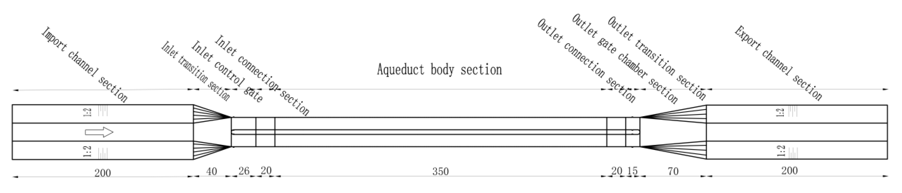
The established three-dimensional model of the aqueduct was established according to the 1:1 model scale. The X-axis direction was selected as the left and right bank direction, with the right bank direction as the X-axis positive direction, the Z-direction was the water depth direction, with the Z-axis negative direction being the gravitational acceleration direction, and the Y-axis was the upstream and downstream direction, with the Y-axis positive direction being the downstream flow direction. As shown in Figure 1 and Figure 2, the total length of the model was 941 m, including 541 m for the aqueduct and 200 m for the inlet and outlet channel sections.

2.2. Governing Equation

The software takes the Navier–Stokes equation as the control equation and uses the Reynolds average method to solve it [16].

Continuity equation:

$$\frac{\partial }{\partial x_i}\left(u_i{A}_i\right)=0$$

(1)

Momentum equation:

$$\frac{\partial u_i}{\partial t}+\frac{1}{V_F}\left({\displaystyle \sum _{j=1}^3{u}_j{A}_j\frac{\partial u_i}{\partial x_j}}\right)=-\frac{1}{\rho }\frac{\partial P}{\partial x_i}+g_i+f_i$$

(2)

where $u_i$ is the direction speed of X, Y, and Z. $A_x$, $A_y$, and $A_z$ are the area of the calculation unit of direction; $V_F$ is the volume fraction of water in each calculation unit; ρ is the density of water; P is the pressure; $g_i$ is gravity; and $f_i$ is the Reynolds stress [17].

Turbulence model:

For RNG k-ε, the model can efficiently solve the flow with large streamline bending [18].

Turbulent kinetic energy equation:

$$\frac{\partial \left(\rho k\right)}{\partial t}+\frac{\partial \left(\rho u_{i}k\right)}{\partial x_i}=\frac{\partial }{\partial x_j}\left(\left(\mu +{\mu }_t\right){\alpha }_k\frac{\partial k}{\partial x_j}\right)+G_k-\rho \epsilon$$

(3)

Turbulent energy dissipation rate equation:

$$\frac{\partial \left(\rho \epsilon \right)}{\partial t}+\frac{\partial \left(\rho u_i\epsilon \right)}{\partial x_i}=\frac{\partial }{\partial x_j}\left(\left(\mu +{\mu }_t\right){\alpha }_{\epsilon }\frac{\partial \epsilon }{\partial x_j}\right)+C_{1\epsilon }^{\ast }\frac{\epsilon }{k}{G}_k-C_{2\epsilon }\rho \frac{{\epsilon }^2}{k}$$

(4)

where k is the turbulent kinetic energy, $\epsilon$ is the turbulent energy dissipation rate, $\mu$ is the hydrodynamic viscosity coefficient, ${\mu }_t$ is the fluid turbulent viscosity, ${\mu }_t=\rho C_{\mu }{k}^2/\mathsf{\epsilon }$, $\mathrm{N}·\mathrm{s}/{\mathrm{m}}^2$; ${\alpha }_{\epsilon },{\alpha }_k$, $C_{1\epsilon }$ and B are constants; ${\alpha }_{\epsilon }$ = ${\alpha }_k$ = 1.39; $C_{1\epsilon }^{*}={\mathrm{C}}_{1\mathsf{\epsilon }}-\eta \left(1-\eta /{\eta }_0\right)/\left(1+\beta {\eta }^3\right)$; $\eta ={\left(2E_{ij}{E}_{ij}\right)}^{0.5}k/\epsilon$; $E_{ij}=1/2\left(\partial u_i/\partial x_j+\partial u_j/\partial x_i\right)$ ${\eta }_0=4.337$; $\beta =0.012$; $C_{1\epsilon }=1.42$; constant $C_{2\epsilon }=1.68$; and $G_k$ is the turbulent kinetic energy generation term caused by the average velocity gradient, $G_k={\mu }_t\left(\partial u_i/\partial u_j+\partial u_j/\partial u_i\right)\partial u_i/\partial u_j$ [19].

2.3. Model Meshing

In this paper, the FLOW-3D software 11.2 was used for meshing, and the mesh was a hexahedral mesh corresponding to the six faces of the 3D model. FLOW3D draws meshes that are divided into structural meshes. It also uses the FAVOR technology to check whether the meshes can be accurately identified with the computational model.

The quality of grid division affects the accuracy of numerical model calculation results. In order to improve the accuracy of the numerical simulation results and to consider the calculation time, the mesh can be optimized and the calculation time costs can be reduced, provided that the results are accurate.

(1)

Grid irrelevance test

In this paper, the irrelevance of a uniform grid with five grid widths of 1.0, 0.9, 0.8, 0.7, and 0.6 m was tested. The grid shape was square. The water depth at the middle of the inlet of the inlet gradient section (point A) was selected for analysis. The numerical simulation results are shown in

Table 1. Simulation results for different grid widths.

Grid Width/m	Total Number of Grids	Number of Fluid Grids	Ending Time/s	Approximate Time of Stabilization/s	Simulated Water Depth at Point A/m
1.0	765,000	426,400	5000	3000	8.236
0.9	987,400	545,700	5000	3000	8.203
0.8	1,395,000	771,000	5000	3000	8.185
0.7	1,915,500	1,045,700	5000	3000	8.183
0.6	2,729,400	1,440,900	5000	3000	8.181

.

As can be seen from Table 1, when the grid size is larger than 0.8 m, the grid width has a greater influence on the simulation results, and the smaller the grid size, the smaller the change in the simulation results; when the grid size is smaller than 0.8 m, the grid width has less influence on the simulation results. Therefore, for the sake of time and accuracy, the grid width in this paper was 0.8 m.

(2)

Grid division

The model was divided following the non-uniform grid method, the important parts of the model were nested, and the local grid was densified. The hydraulic characteristics of the inlet and outlet transition sections were the focus of this paper. Nested grid processing was carried out for the positions of the entrance and exit transition sections and the vicinity of the middle pier of the exit transition section. The nested grid of the model exit transition section area is shown in Figure 3. The nested grid area of the exit transition section was as follows: X axis (−10 m–10 m), Y axis (650 m–741 m), Z axis (−2.5 m–9.76 m), and the grid division size was 0.5 m. The nested grid area of the entrance transition section was as follows: X axis (−10 m–10 m), Y axis (200 m–260 m), Z axis (−2.5 m–9.76 m), and the grid size was 0.5 m. The overall mesh size was 0.8 m and the total number of grids was 1.395 million.

2.4. Setting of Model Boundary Conditions and Initial Conditions

(1) Boundary condition setting

The upstream inlet boundary condition of the model was set as the flow inlet boundary. The downstream outlet boundary condition of the model was set as the pressure outlet boundary, and the water level corresponding to each simulated working condition was provided. The wall boundary was provided at the left and right banks (positive and negative directions of the X-axis) and at the bottom of the model (negative direction of the Z-axis). The pressure outlet was provided at the top of the model (positive direction of the Z-axis), where the fluid fraction was set to 0; that is, the top of the model was atmospheric pressure.

(2) Initial condition setting

It can be seen from Figure 2 that the total length of the calculation model was 941 m. If the initial conditions of the model do not provide the corresponding initial water level according to the simulation conditions, and the tank runs empty, the calculation time will be increased. If only the initial water level is given, the water flow in the tank will oscillate during the simulation, and it will take a long time for the model to stabilize, therefore, on the basis of the given water level, an average flow rate is provided for the initial water body according to the simulation conditions to reduce the oscillation and improve the calculation efficiency. In order to clearly and accurately determine the stability of the model calculation, monitoring sections were set up upstream and downstream of the inlet and outlet to observe the flow and velocity changes of specific sections. When the difference between the instantaneous changes in flow is very small, the model calculation is stable [20].

3. Model Validation

3.1. Comparison of Measured Data of Model Calculation Results

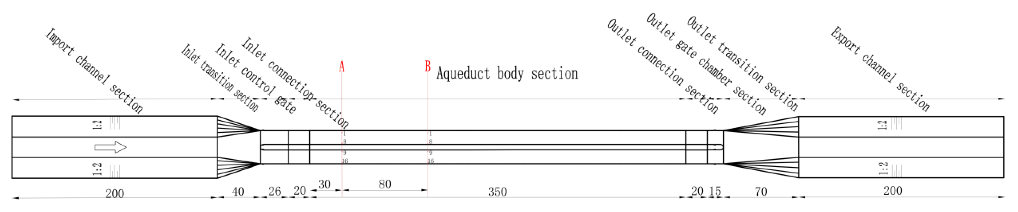
Relevant staff carried out field measurements of the typical drains studied in this paper from 11:00 to 14:00 on 29 August 2019. The instantaneous flow was 227.68 m³/s. The water level on the left bank in front of the gate was 147.00 m and the water depth was 8.20 m; The water level on the right bank in front of the gate was 146.90 m and the water depth was 8.18 m. When measuring the velocity of the aqueduct on site, the first cross section of the aqueduct along the water flow direction was section A and the second cross section was section B. Measuring points were arranged along the right side of section A; 1 measuring point was arranged every 1 m, 12 measuring points were arranged in each channel body, and a total of 24 measuring points were arranged in the two tanks. The arrangement of the measuring points is shown in Figure 4.

Simulation parameters were set according to the analysis of the measured data. The measured flow was 227.68 m³/s. The inlet flow boundary was set with a flow of 227.68 m³/s. The water level at the outlet pressure boundary was 146.33 m. The initial water level of the model was 146.33 m. The initial velocity was 0.8 m/s. The channel roughness was set at 0.014. The calculation time was set to 5000 s. The initial time step was set to 0.002 s, and the minimum time step was set to 1 × 10⁻⁸ s. This paper selected the RNG k-ε turbulence model.

It can be seen from the comparison between the measured water depth and the simulated water depth on the left and right banks of the aqueduct in

Table 2. Comparison between measured water depth and simulated water depth on the left bank of the aqueduct.

Left Bank Section of Aqueduct Body Section
Measuring point	L1	L2	L3	L4	L5	L6
Measured water depth	5.63	5.7	5.78	5.71	5.62	5.77
Simulated water depth	5.58	5.68	5.75	5.75	5.67	5.71
Measuring point	L7	L8	L9	L10	L11	L12
Measured water depth	5.64	5.78	5.74	5.77	5.63	5.70
Simulated water depth	5.58	5.73	5.68	5.71	5.72	5.76

and

Table 3. Comparison between measured water depth and simulated water depth on the right bank of the aqueduct.

Right Bank Section of Aqueduct Body Section
Measuring point	R1	R2	R3	R4	R5	R6
Measured water depth	5.65	5.77	5.80	5.71	5.74	5.65
Simulated water depth	5.60	5.70	5.74	5.76	5.69	5.61
Measuring point	R7	R8	R9	R10	R11	R12
Measured water depth	5.79	5.66	5.74	5.80	5.64	5.77
Simulated water depth	5.73	5.62	5.68	5.75	5.7	5.69

that the water depth at different positions in the aqueduct body fluctuated, indicating that the numerical simulation could reflect the actual situation. The maximum difference in water depth was 0.07 m and the percentage of error in the measured water depth was 1.2%, which was consistent with the trend of the measured water depth data. By comparing the measured water depth and velocity with those of the numerical simulation, it could be seen that the parameter values and the numerical model establishment and solution results were reliable.

3.2. Setting of Simulated Working Conditions

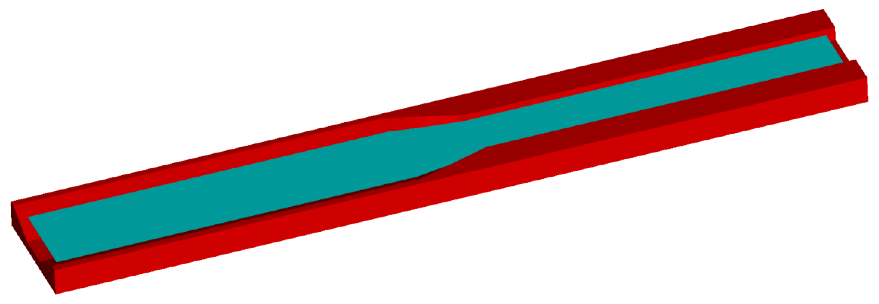
In this paper, the study was carried out on the inlet tapering section of the aqueduct, and a three-dimensional numerical model of the inlet tapering section of the aqueduct was constructed as in Figure 5 without affecting the accuracy of the numerical simulation. A value of 200 m was taken for the upstream open channel section of the inlet tapering section, and 200 m was taken for the downstream channel body section of the tapering section.

As shown in

Table 4. Values of W_up and W_down for the models’ working conditions.

Model Number	Wup (m)	Wdown (m)	Model Number	Wup (m)	Wdown (m)
1	19	31	4	28	31
2	22	31	5	31	31
3	25	31	6	34	31

, this paper considered the influence of the bottom width ratio of the inlet and outlet of the inlet and outlet tapering sections, and set a total of six model conditions; the simulation types included inlet W_up/W_down < 1, model number 1–4; W_up/W_down = 1, model number 5; and W_up/W_down > 1, model number 6. The model conditions were selected to reflect the influence of W_up/W_down on the overflow capacity. The water level and flow rate of each model condition were set as shown in

Table 5. Simulated water level for each operating condition (expressed as pressure).

Work Conditions	Inlet Pressure Pin (m)	Outlet Pressure Pout (m)	Work Conditions	Inlet Pressure Pin (m)	Outlet Pressure Pout (m)
1	4.8	4.5	5	6.8	6.5
2	5.3	5.0	6	7.3	7.0
3	5.8	5.5	7	7.8	7.5
4	6.3	6.0	8	8.3	8.0

, and eight water level and flow rates are set for each model condition.

4. Analysis of Simulation Results

In the energy equation, asymptotic section head loss is mainly local head loss; this study did not consider the head loss along the asymptotic section to calculate the local head loss. According to the simulation results, we could derive the upstream and downstream overwater area of the inlet gradient section, as well as derive the water surface contraction angle θ (the angle between the edge of the water surface at the transition section and the centerline). The model working condition was W_up = 19 m and W_down = 31 m, and the simulation working condition 1 results are shown in

Table 6. Weir head under simulated working conditions.

Water Level (m)	Angle (°)	Water Depth of Tank (m)	Downstream Area (m2)	Upstream Water Depth (m)	Upstream Area (m2)	Head Loss Coefficient
8.3	14.84	6.184	191.704	8.220	291.291	0.280
7.8	13.5	5.695	176.542	7.724	266.081	0.311
7.3	12.13	5.194	161.002	7.221	241.485	0.339
6.8	10.76	4.705	145.867	6.729	218.392	0.383
6.3	9.37	4.206	130.374	6.225	195.789	0.420
5.8	7.97	3.715	115.168	5.732	174.615	0.464
5.3	6.56	3.225	99.963	5.236	154.331	0.527
4.8	5.14	2.750	85.241	4.745	135.193	0.593

.

As can be seen above, Nguyen et al. experimentally determined the head loss coefficient of a rectangular open channel to a rectangular abruptly constricted pressurized pipe. A head loss coefficient of $\mathsf{\zeta }$ = 0.63 (1 − A_down/A_up) was obtained, and A_up and A_down were the upstream and downstream cross-sectional over-water areas, respectively. Tokyay fitted the local head loss expression $\mathsf{\zeta }=0.74{\left(\mathsf{\Delta }\mathrm{z}/{\mathrm{h}}_1\right)}^{0.5}$ for a 45° inclined negative step flow via an experimental study; h₁ was the downstream water depth and $\mathsf{\Delta }\mathrm{z}$ was the difference in the elevation of the bottom surface of the inlet gradient section. In this paper, through the analysis of the simulation results and taking into account the effects of the water surface contraction angle and the upstream and downstream cross-sectional areas of the gradient section, the expression of the head loss coefficient of the gradient section can be given on the basis of existing research [5].

$$\mathsf{\zeta }=\frac{\mathsf{\theta }}{90}{\left(1-\frac{{\mathrm{A}}_{\mathrm{down}}}{{\mathrm{A}}_{\mathrm{up}}}\right)}^{{\mathrm{x}}_1}+{\mathrm{x}}_2{\left(\mathsf{\Delta }\mathrm{z}/{\mathrm{h}}_1\right)}^{{\mathrm{x}}_3}$$

(5)

Substituting the results of W_up/W_down = 19/31 simulated working conditions into Equation (5), we get: coefficients x₁ = 20.755, x₂ = 0.837, and x₃ = 0.891, and the correlation coefficient is 0.995.

As shown in

Table 7. Weir head under the simulated working conditions.

Wup/Wdown	Angles (°)	Local Head Loss Coefficient	Wup/Wdown	Angles (°)	Local Head Loss Coefficient	Wup/Wdown	Angles (°)	Local Head Loss Coefficient
19/31	14.84	0.280	22/31	16.83	0.249	25/31	18.78	0.222
	13.5	0.311		15.51	0.273		17.48	0.247
	12.13	0.339		14.17	0.292		16.17	0.263
	10.76	0.383		12.82	0.323		14.84	0.292
	9.37	0.420		11.45	0.357		13.5	0.319
	7.97	0.464		10.07	0.400		12.13	0.358
	6.56	0.527		8.67	0.451		10.76	0.406
	5.14	0.593		7.27	0.513		9.37	0.468
28/31	20.68	0.211	31/31	22.54	0.201	34/31	24.35	0.191
	19.42	0.232		21.31	0.223		23.15	0.217
	18.13	0.246		20.05	0.236		21.92	0.227
	16.83	0.281		18.78	0.262		20.68	0.255
	15.51	0.298		17.48	0.284		19.42	0.272
	14.17	0.335		16.17	0.323		18.13	0.310
	12.82	0.380		14.84	0.364		16.83	0.350
	11.45	0.440		13.5	0.424		15.51	0.410

, the simulation results of each model condition were analyzed.

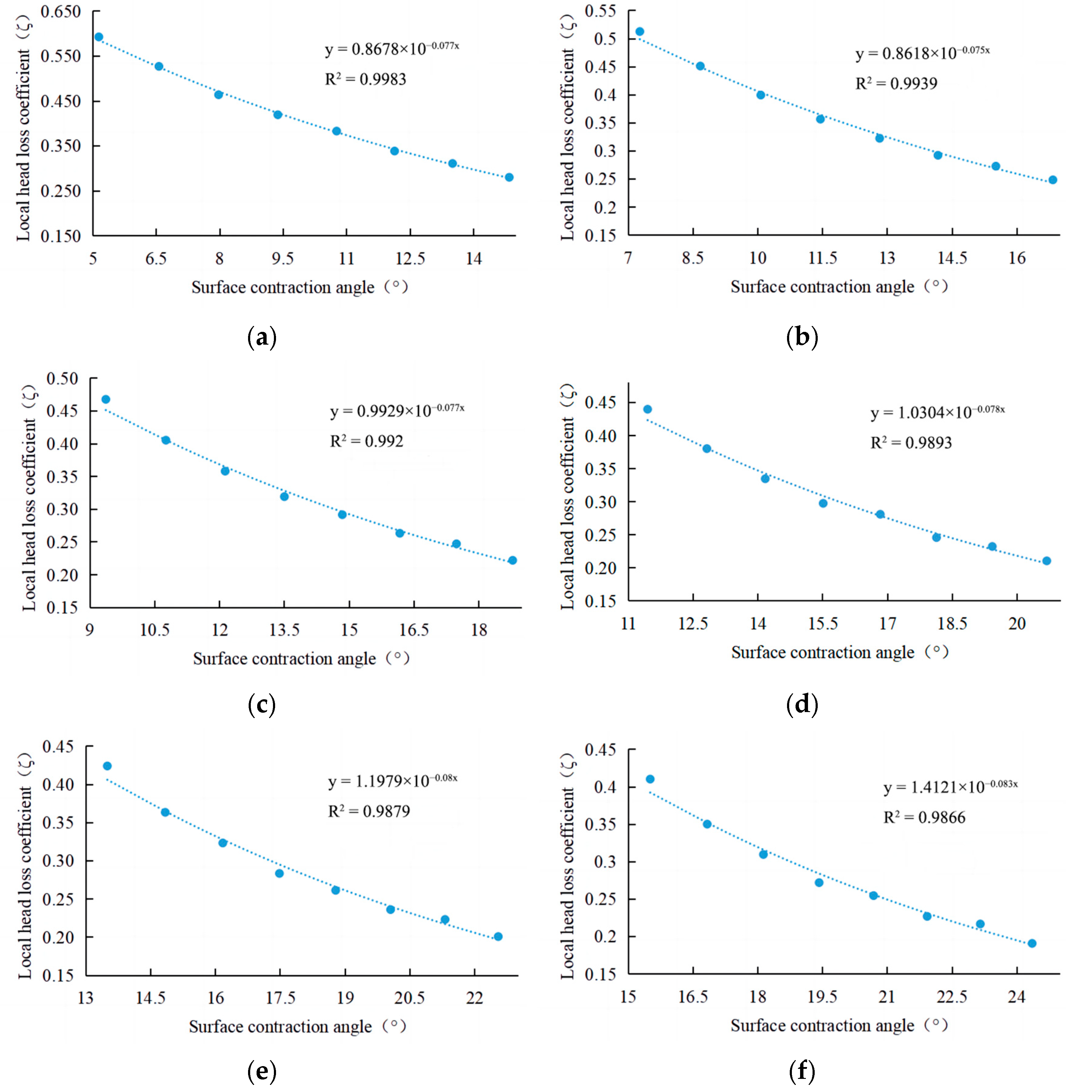
As shown in Figure 6, the local head loss coefficient of each model condition decreased with the increase in the water surface contraction angle, and the local head loss coefficient corresponding to the same water surface contraction angle also increased with the increase in W_up/W_down. The water surface contraction angle θ (°) and the local head loss coefficient had a good exponential function relationship that met $\mathsf{\zeta }={\mathsf{\alpha }\mathrm{e}}^{\mathsf{\beta }\left({\mathrm{W}}_{\mathrm{up}}/{\mathrm{W}}_{\mathrm{down}}\right)}$, where α and β are the formula coefficient terms and the correlation coefficients R² of each model condition fit were above 0.98.

As shown in Figure 7, the nonlinear regression analysis of W_up/W_down with exponential function $\mathsf{\zeta }={\mathsf{\alpha }\mathrm{e}}^{\mathsf{\beta }\left({\mathrm{W}}_{\mathrm{up}}/{\mathrm{W}}_{\mathrm{down}}\right)}$ was performed for each model working condition. W_up/W_down had a good one-to-one quadratic function relationship with coefficient α, and the correlation coefficient R² was 0.9996; W_up/W_down had a good one-to-one quadratic function relationship with coefficient β, and the correlation coefficient R² was 0.9577.

Through the above analysis, the local head loss coefficient of the inlet tapering section of the aqueduct was written as an exponential function relationship, $\mathsf{\zeta }={\mathsf{\alpha }\mathrm{e}}^{\mathsf{\beta }\left({\mathrm{W}}_{\mathrm{up}}/{\mathrm{W}}_{\mathrm{down}}\right)}$, related to the water surface contraction angle in the tapering section, and coefficients α, β, and W_up/W_down had a one-dimensional quadratic function relationship. In order to verify the accuracy and applicability of the formula, the formula was used to solve the local head loss coefficient when W_up/W_down was 19/31 and the water surface contraction angle was 10.76°. The formula calculated the local head loss coefficient to be 0.3796, the simulated value was 0.383, the error was 3.4 × 10⁻³, and the error percentage was 0.89%.

5. Conclusions

In this paper, the following conclusions were obtained from a three-dimensional simulation study of a typical aqueduct.

(1) After the shape of the inlet tapering section was determined, the head loss coefficient ζ was related to the area of the overwater section of the inlet and outlet of the tapering section, the contraction angle of the water surface of the tapering section, and the difference in elevation of the bottom surface of the inlet and outlet of the tapering section. On the basis of existing research results, the local head loss coefficient was provided to meet the functional form of $\mathsf{\zeta }=\frac{\mathsf{\theta }}{90}{\left(1-\frac{{\mathrm{A}}_{\mathrm{down}}}{{\mathrm{A}}_{\mathrm{up}}}\right)}^{{\mathrm{x}}_1}+{\mathrm{x}}_2{\left(\Delta \mathrm{z}/{\mathrm{h}}_1\right)}^{{\mathrm{x}}_3}$, where x₁, x₂, and x₃ are the formula’s coefficients.

(2) The study and analysis of different bottom widths Wup/Wdown of the inlet gradient section showed that the local head loss coefficient decreased with the increase in the water surface contraction angle, and with the increase in W_up/W_down, the local head loss coefficient corresponding to the same water surface contraction angle also increased; the local head loss coefficient had a good exponential function relationship with W_up/W_down, which satisfied the functional form $\mathsf{\zeta }={\mathsf{\alpha }\mathrm{e}}^{\mathsf{\beta }\left({\mathrm{W}}_{\mathrm{up}}/{\mathrm{W}}_{\mathrm{down}}\right)}$, where α and β are the formula’s coefficients.

6. Patents

This section is not mandatory but may be added if there are patents resulting from the work reported in this manuscript.

References

- Wang, Z. Von Karman and Karman Vortex Street. Nat. J. 2010, 32, 243–245. [Google Scholar]
- Li, W. Hydraulic Calculation Manual, 2nd ed.; Water Conservancy and Hydropower Press: Beijing, China, 2006. [Google Scholar]
- SL 482-2011; Specification for the Design of Irrigation and Drainage Canal System Buildings. Ministry of Water Resources of the People’s Republic of China: Beijing, China, 2011.
- Zhai, Y. Study on the calculaion method of local head loss in the gradual change section of the main trunk canal of the South-North Water Diversion Project. J. Irrig. Drain. 2007, 26 (Suppl. S1), 20–22. [Google Scholar] [CrossRef]
- Wu, Y.Y.; Liu, Z.W.; Chen, Y.C. Flow characteristics and minor losses in transition section from trapezoidal open channel to horseshoe-shaped tunnel. J. Hydroelectr. Eng. 2016, 35, 46–55. [Google Scholar]
- Wang, S. Study on Water Level Fluctuation Mechanism and Control Measures of Large Aqueduct in Middle Route Project of South to North Water Diversion; North China University of Water Resources and Electric Power: Zhengzhou, China, 2021. [Google Scholar] [CrossRef]
- Qu, Z.; Lim, Z. Causal analysis on water level abnormal fluctuation in aqueduct and improvement measures:case of Lihe aqueduct in Middle Route of South to North Water Transfer Project. Yangtze River 2022, 53, 189–194. [Google Scholar] [CrossRef]
- Kazemipour, A.K.; Apelt, C.J. Resistance to Flow in Irregular Channels; Department of Civil Engineering, University of Queensland: Brisbane, Australia, 1980. [Google Scholar]
- Henderson, F.M. Open Channel Flow; McMillan Book Company: New York, NY, USA, 1966. [Google Scholar]
- Chow, V.T. Open-Channel Hydraulics; McGraw-Hill: New York, NY, USA, 1959. [Google Scholar]
- Yaziji, H.M. Open-Channel Contractions for Subcritical Flow; The Univeristy of Arizonam: Tucson, AZ, USA, 1968. [Google Scholar]
- Zhang, Z. Hydraulic Design of the Inlet and Outlet Connection Section of a Pressureless Tunnel; Shanxi Water Resources: Xi’an, China, 1991; pp. 34–40. [Google Scholar]
- Gaetano, C.; David, D.; Corrado, G.; Michael, P. Hydraulic Capacity of Bend Manholes for Supercritical Flow. J. Irrig. Drain. Eng. 2023, 149, 04022048. [Google Scholar]
- Cheng, Y.; Song, Y.; Liu, C.; Wang, W.; Hu, X. Numerical Simulation Research on the Diversion Characteristics of a Trapezoidal Channel. Water 2022, 14, 2706. [Google Scholar] [CrossRef]
- Tellez-Alvarez, J.; Gómez, M.; Russo, B.; Amezaga-Kutija, M. Numerical and Experimental Approaches to Estimate Discharge Coefficients and Energy Loss Coefficients in Pressurized Grated Inlets. Hydrology 2021, 8, 162. [Google Scholar] [CrossRef]
- Qi, L.; Chen, H.; Fei, W.; Dong, L. Three-dimensional numerical simulations of flows over spillway dam using accurate river terrain. J. Hydroelectr. Eng. 2016, 35, 12–20. [Google Scholar]
- Wang, Y.; Bao, Z.; Wang, B. Three-dimensional numerical simulation of flow in stilling basin based on Flow-3D. Eng. J. Wuhan Univ. 2012, 45, 454–457+476. [Google Scholar]
- Ran, D.; Wang, W.; Hu, X.; Shi, L. Analyzing hydraulic performance of trapezoidal cutthroat flumes. Adv. Water Sci. 2018, 29, 236–244. [Google Scholar]
- Xiao, Y.; Wang, W.; Hu, X. Numerical simulation of hydraulic performance for portable short-throat flume in field based on FLOW-3D. Trans. Chin. Soc. Agric. Eng. 2016, 32, 55–61. [Google Scholar]
- Guan, G.; Huang, Y.; Xiong, J. Uniform flow rate calibration model for flat gate under free-submerged orifice flow. Trans. Chin. Soc. Agric. Eng. 2020, 36, 197–204. [Google Scholar]
Figure 1.
Aqueduct floor plan.
Figure 2.
Three-dimensional layout of the aqueduct.
Figure 3.
Grid division. (a) Export gradient segment local encryption; (b) Model meshing.
Figure 4.
Layout of measuring points on a typical aqueduct.
Figure 5.
Prototype inlet gradient section model diagram.
Figure 6.
Each model working condition water surface contraction angle as a function of the local head loss coefficient. (a) θ as a function of ζ at Wup/Wdown 19/31; (b) θ as a function of ζ at Wup/Wdown 22/31; (c) θ as a function of ζ at Wup/Wdown 25/31; (d) θ as a function of ζ at Wup/Wdown 28/31; (e) θ as a function of ζ at Wup/Wdown 31/31; (f) θ as a function of ζ at Wup/Wdown 34/31.
Figure 7.
Wup/Wdown as a function of coefficient. (a) Wup/Wdown as a function of coefficient α; (b) Wup/Wdown as a function of coefficient β.