
Application of Deep Learning in Drainage Systems Monitoring Data Repair—A Case Study Using Con-GRU Model
by
 ,
,
Li He
1,
Shasha Ji
1,
Kunlun Xin
2,3,
Zewei Chen
1,
Lei Chen
2,3,*,
Jun Nan
4,* and
Chenxi Song
1 1
Shanghai Urban Construction Design and Research Institute, Shanghai 200125, China
2
College of Environmental Science and Engineering, Tongji University, Shanghai 200092, China
3
Smart Water Joint Innovation R&D Center, Tongji University, Shanghai 200092, China
4
School of Environment, Harbin Institute of Technology, Harbin 150090, China
*
Authors to whom correspondence should be addressed.
Water 2023, 15(8), 1635; https://doi.org/10.3390/w15081635
Submission received: 19 February 2023
/
Revised: 6 April 2023
/
Accepted: 19 April 2023
/
Published: 21 April 2023
(This article belongs to the Section Urban Water Management)
Abstract
:Hydraulic monitoring data is critical for optimizing drainage system design and predicting system performance, particularly in the establishment of data-driven hydraulic models. However, anomalies in monitoring data, caused by sensor failures and network fluctuations, can severely impact their practical application. Such anomalies can persist for long periods, and existing data repair methods are primarily designed for short-term time series data, with limited effectiveness in repairing long-term monitoring data. This research introduces the DSMDR, a deep learning framework designed for repairing monitored data in drainage systems. Within this framework, a deep learning model named Con-GRU is proposed for repairing water level monitoring data with long-term anomalies (i.e., 288 consecutive time points) in the pump station forebay. The model iteratively predicts 36 time points at each iteration and uses an iterative approach to achieve the repair process for long-term abnormal monitoring data. The Con-GRU model integrates analysis of forebay water levels, pump status, and rainfall features related to repair, and captures both long-term and local time-dependent features via one-dimensional convolution (Conv1D) and gated recurrent units (GRU). The proposed model improves the accuracy and authenticity of repaired water level data. The results indicate that, compared to existing long short-term memory neural network (LSTM) and artificial neural network (ANN) models, the Con-GRU model has significantly better performance in repairing water level data.
1. Introduction
The urban drainage system plays an indispensable role in urban infrastructure development by safeguarding environmental sanitation, improving residents’ quality of life, mitigating flood damages, and enhancing water resource management efficiency. In recent years, the development of the internet of things (IoTs) has provided the possibility for data collection, transmission, analysis, and application, and has also laid the foundation for the development of urban drainage systems; the collection of extensive drainage monitoring data has facilitated the progress of smart water management [1]. The application of advanced information technologies, such as artificial intelligence and big data analytics, in the framework of smart water management, enables the processing and analysis of drainage monitoring data, leading to the automation and optimization of drainage system management and control. As a result, the efficiency of water management and the decision-making capabilities of water management authorities are improved. The key of data analysis is to identify the inherent features within the monitored data, which imposes additional requirements on the quality of drainage data. High-quality drainage data can provide accurate information, support effective decision-making and planning, and be used to predict future demands and challenges for the system. As a critical component of the development of smart water, a large amount of drainage monitoring data is required to guarantee the precision of the model in practical situations. However, real-time monitoring data often contains many abnormal values, which can drastically impact the results of data analysis and modeling [2]. These abnormal data may come from all aspects of data collection, transmission, and recording [3,4]. The main causes of abnormal data are sensor damage, harsh deployment environment, network transmission failure, and the environmental noise, etc. [5,6,7,8]. It is important to ensure the continuity and applicability of data to detect and repair the abnormal values in real-time monitoring data.
Statistical methods [9,10,11], machine learning methods [12,13,14], and deep learning methods [15,16,17,18] based on data analysis and data mining have been applied to the anomaly detection of time series, and the anomaly detection performance has been greatly improved. In the field of water management, the above methods have been widely used in the anomaly detection of hydrological time series data, in recent years [19,20,21,22]. However, simply discarding the abnormal values of time series results in a lack of temporal continuity. Moreover, when the time series data contains a large number of continuous abnormal values, the model based on the time series with a large number of eliminated continuous abnormal values is unreliable [2]. How to repair such continuous abnormal values, so as to ensure the accuracy of hydraulic model calibration, is key to the establishment and application of drainage system models.
Xu et al. [23] proposed a spatial-temporal point interpolation method to perform linear unbiased estimation of missing values to repair air quality monitoring data. Wang et al. [24] proposed a hybrid missing data imputation framework to repair missing values in traffic flow data, by analyzing and mining periodic patterns. Park et al. [25] proposed a LightGBM model based on a sliding window, using the random forest method to repair short-term electricity load data. In the above research, statistical analysis and machine learning methods are used to repair time series monitoring data, which are often based on the assumption that the data conforms to a certain distribution, thus limiting the accuracy of data repair. With the development of science and technology, deep learning methods, including models such as recurrent neural network (RNN) and convolutional neural network (CNN), have been applied in all aspects of the drainage field, including sewer defect and blockage detection [26], urban flood forecasting [27], flood control of urban systems [28], wastewater treatment plants [29], and rainfall-runoff forecasting [30,31,32,33]. Similarly, deep learning has been applied to the repair of time series abnormal values in recent years. Song et al. [34] constructed a long short-term memory (LSTM) data repair model for the stem moisture data of plants, and proved that it has great advantages in repairing long-term missing values of time series data. In the field of water management, Ren et al. [35] constructed a repair model of subsurface hydrological flow data based on LSTM, and concluded that it has stronger data repair capabilities than the ARIMA model. Lattawit et al. [36] proposed an LSTM interpolation method suitable for repairing various types of hydrological time series data, and proved that its effect on the distinct tidal data pattern is better than other methods. From the above research, it can be seen that the principle of using deep learning methods to repair time series monitoring data is to build a deep learning model to predict and fill abnormal data points to achieve the effect of repair, but there are still some gaps in the current research: (1) The time series repair models based on deep learning are mostly single-step prediction models. When such models are used for data repairing, iterative prediction is needed to realize the repair of multistep time series, which will lead to the accumulation of prediction errors, thus affecting the effect of data repair. (2) The direct multistep prediction repair model, based on deep learning, has the problem of insufficient prediction accuracy, and the length of data to be repaired in the time series is not fixed, which also increases the difficulty of setting the prediction step. (3) Most of the existing research only models the repaired time series feature, ignoring that the repaired data is often affected by other features, such as humidity being affected by rainfall, etc.
In the urban drainage system, the continuous measurements of the hydraulic environment and operating status recorded by sensors can be considered as time series data, which include water level, pump status, humidity, and so on. In order to advance the progress of deep learning technology in repairing hydraulic monitoring data of drainage systems, this research takes the water level monitoring data of the forebay as the object. The forebay is an important part of the sewage inlet design of the pumping station project. Its water level monitoring data determines the opening and closing status of the rainwater pumps and sewage pumps, thus affecting the operation of the entire drainage system. Conversely, the status of the pumps will also affect the change of the water level. In addition, the forebay water level is also closely related to rainfall. Therefore, the water level monitoring data of the forebay can reflect the operation of the entire drainage system, and its accuracy is the basis for the establishment and calibration of the hydraulic model. The aims of this research are: (1) to propose a long-term anomalous time series repair model, Con-GRU, based on multistep iterative prediction; (2) to investigate the impact of different features, such as pump status and rainfall, on data repair; and (3) to explore the effect of different deep learning model structures on data repair. To demonstrate the capability of the proposed model, the results are compared with those from LSTM and ANN models.
2. Materials and Methods
2.1. Process Framework
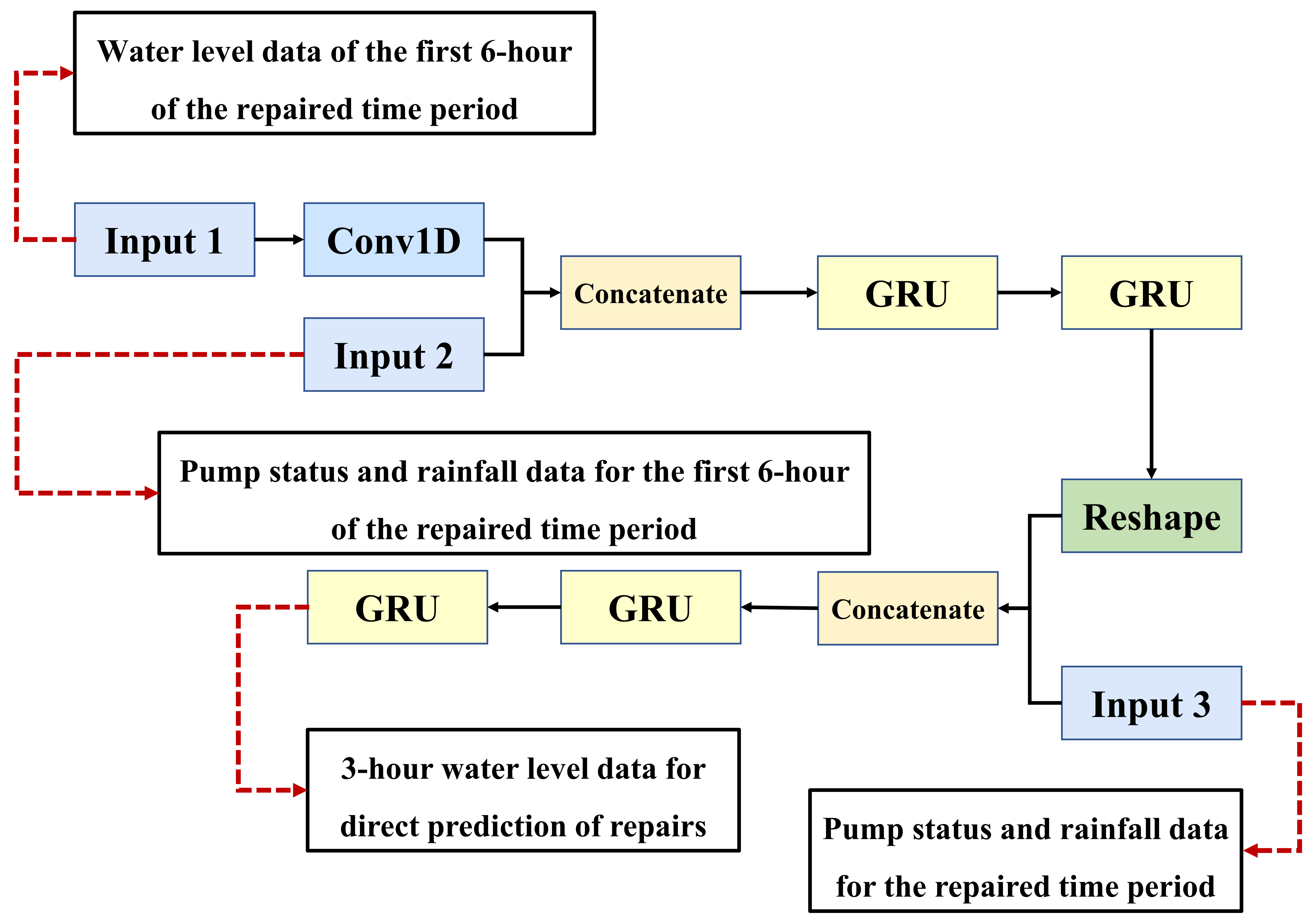
In this research, a framework of drainage system monitoring data repair (DSMDR) is proposed, which can be divided into three parts, as shown in Figure 1.
The first part concerns constructing the dataset. In this process, the sensor data S that needs to be repaired is first identified, and then other sensor monitoring data F that is closely related to S is analyzed. Subsequently, these two elements are used to construct the dataset D for data repair. Finally, the dataset D is partitioned into training, validation, and test datasets according to certain principles. The training dataset is used for model training, while the validation dataset is used to prevent overfitting or underfitting during the training process. Lastly, the test dataset is employed to evaluate the practical application of the model on unknown datasets. The second part comprises the establishment and training of the model. In this regard, considering that this research aims to repair long-term abnormal monitoring data using an iterative prediction approach, the sequence length OL repaired by the model needs to be set. Furthermore, to ensure the effectiveness of each iteration, the appropriate sequence input length IL of the model needs to be determined, as described in Section 3.3. In addition, a suitable deep learning model is constructed based on the number of input features determined in the first part, as presented in Section 3.4. After constructing the model, the training dataset is utilized for model training, while the validation dataset is employed to ensure the efficacy of the model training. The third part involves model testing and application. In this process, the test dataset is used to test the model, evaluating the effectiveness of both single-step and multistep iterative repairs. For single-step iterative repair, the model uses actual monitoring data in each repair iteration, as describe in Section 4.1. For multistep iterative repair, only actual monitoring data is used in the initial iteration, whereas the repaired results are used to update the model input in subsequent iterations, facilitating long-term abnormal data repair, as describe in Section 4.2 and Section 4.3.
2.2. One-Dimension Convolution (Conv1D)
A convolutional neural network (CNN) [37,38] is a type of feedforward neural network that utilizes multiple convolution and pooling operations to progressively extract features from the input data and generate robust features that are resistant to translation deformations. As the number of layers in the network increases, the extracted features tend to become more abstract.
A typical convolutional neural network usually consists of input layers, convolutional layers, pooling layers, fully connected layers, and output layers [39]. The input data is usually two-dimensional image data, since the CNN is originally designed to process image information. The reason CNN performs well on machine vision problems lies in the convolution operation of its convolutional layers. The convolution layer consists of various types of convolution kernels. In the process of convolution, each kind of convolution kernel and the convolved part of the data are convolved to obtain the extracted features, and perform modular representation. The lower convolution layers can extract global features, while the higher convolution layers can extract more abstract and representative features. In addition, the characteristics of local perception and parameter sharing of CNN also improve its application ability in practice. These advantages also make it particularly effective for time series processing, where time can be viewed as a spatial dimension, such as the height or width of a two-dimensional image [40].
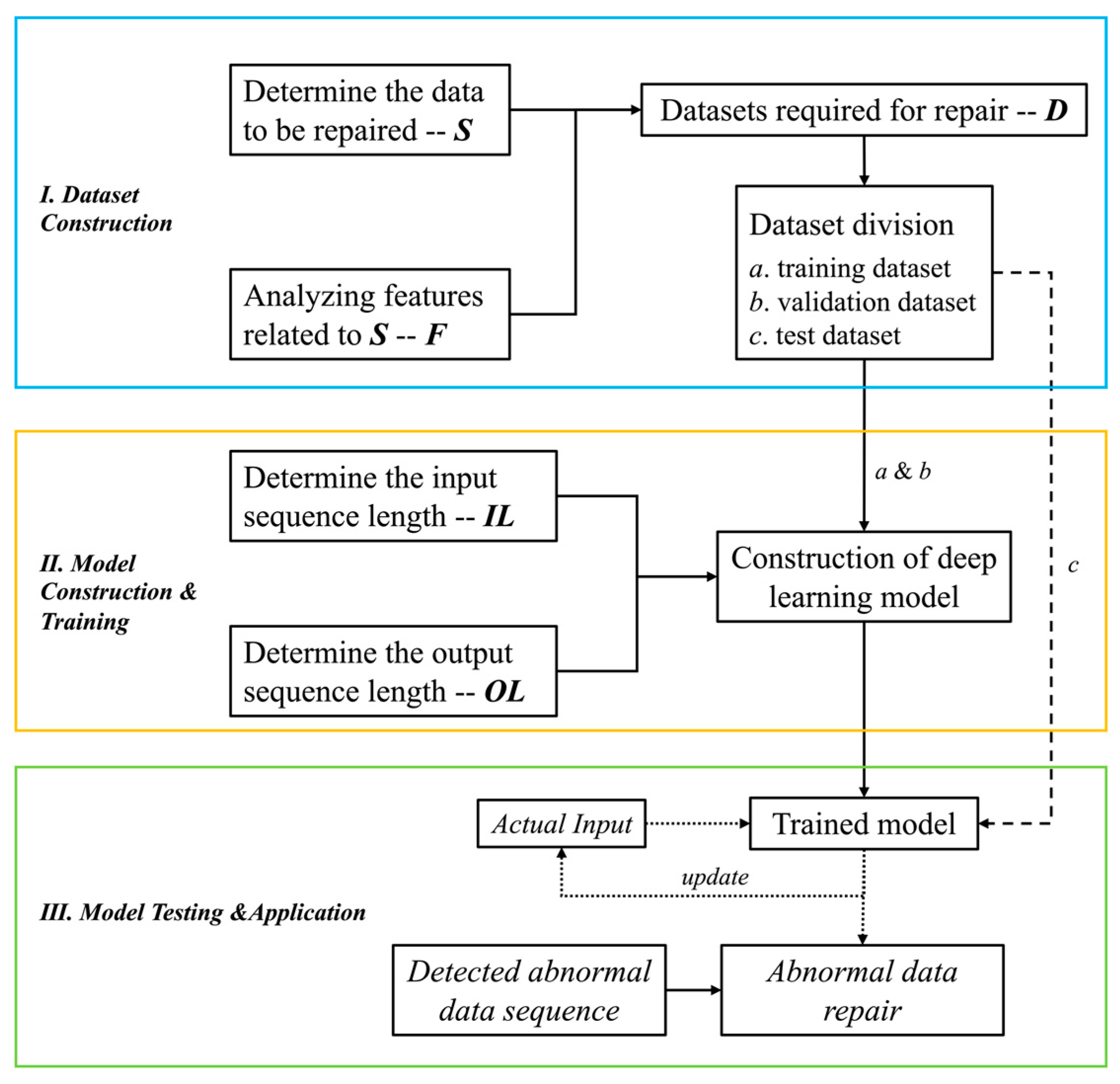
In order to better apply convolution to time series applications, one-dimensional convolution (Conv1D) is used. Conv1D is a convolution operation specially used to process time series data. It has only one spatial dimension, which is more suitable for feature extraction of drainage monitoring data. Conv1D achieves feature extraction by moving a fixed-size sliding window on the input sequence and performing an inner product operation at each window position to generate an output sequence [41]. The process of convolution operation is shown in Figure 2.
The convolution calculation can be expressed by the following Equation (1):
where, is the input data; is the output data; is the convolution kernel weight; is the convolution kernel bias; is the activation function.
2.3. Gated Recurrent Unit (GRU)
Unlike feedforward neural networks, recurrent neural networks (RNNs) [42] are designed to process sequential data, such as time series data. RNNs have the ability to “remember” past information, which allows them to effectively capture time-dependent features in the input data. Instead of processing the input data as a single batch, RNNs iterate over each element in the sequence and store the learned information in a state, allowing them to effectively process time series data.
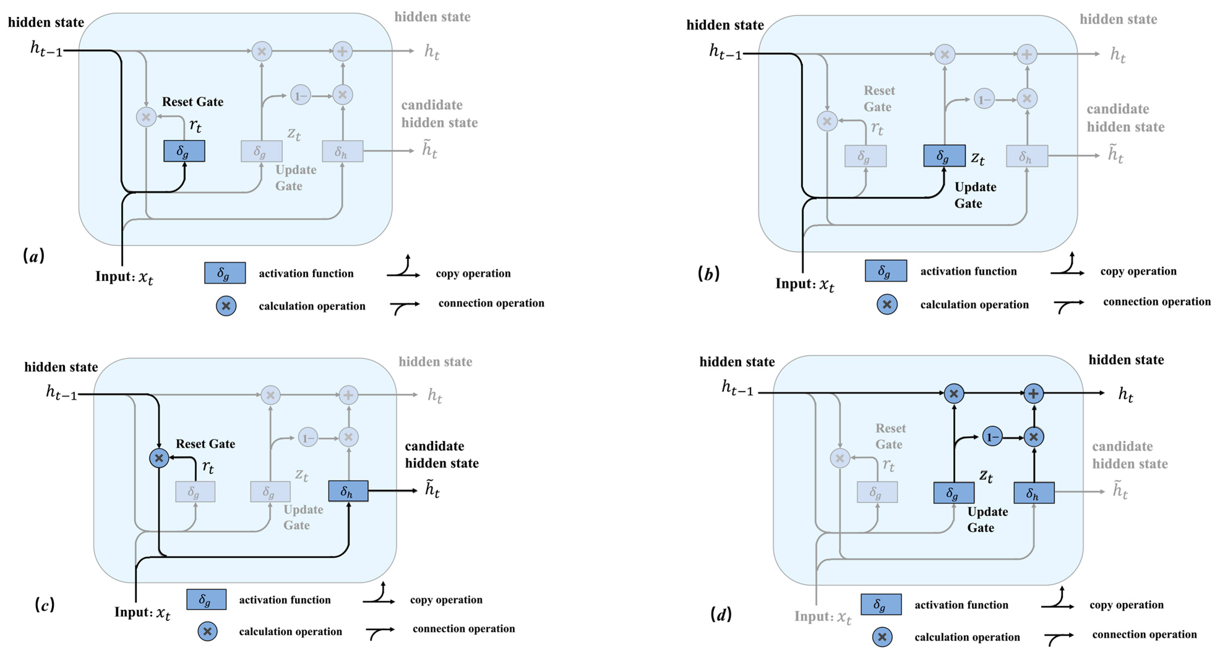
The gated recurrent unit (GRU) [43] is a variant of an RNN that is designed to address the problem of vanishing gradients, which can occur when training deep RNNs. This problem can make the network difficult or impossible to train as the number of layers increases. To solve this problem, the GRU introduces a gating mechanism that controls the flow of information across multiple time steps, allowing it to effectively retain important signals and prevent them from fading away during processing. By setting update and reset gates, the GRU is able to improve its ability to select relevant features. The calculation process for the GRU is illustrated in Figure 3.
The principles of the four processes in Figure 3 are expressed by Equations (2)–(5):
where, is the update gate; is the reset gate; , , and are parameters for weights and bias; is the hidden state; is the candidate hidden state; is the sigmoid function; is the tanh function; is the current calculation time step. The values of and are both in the range from 0 to 1.
2.4. Data Sample Generation Strategy
The ability of neural networks to learn the relationship between input and output is a key factor in their success. As such, it is important to have a large number of data samples that correspond to input and output pairs when training a neural network. One common method for constructing such samples is the sliding window scheme, which is widely used in supervised learning for neural networks [44].
The sliding window scheme is a useful technique for extracting dynamic features from large-scale time series data. It works by treating the data within a sliding window as a subsequence. For a time series dataset , the sliding window scheme can be used to divide the original time series into multiple subsequences of equal length, with the number of subsequences given by Equation (6). This is particularly useful for ensuring that the number of elements in each subsequence remains constant as the sliding window is updated over the time series data.
where, is the number of subsequences; is the length of original time series data; is the width of sliding window; , is the length of input, 72 in this research; is the length of output, 36 in this research; is the move length of the sliding window for each update, 1 in this research.
2.5. Model Establishment Strategy
This research focuses on repairing the water level data of the pumping station forebay. As water level data is time series data, the approach to repairing abnormal data involves predicting the data for the abnormal time period, and using the predicted normal values to backfill and correct the abnormal data.
There are several factors that can impact the water level in the forebay of the pumping station. Firstly, in the absence of rainfall, the water level tends to increase due to the discharge of domestic sewage into the drainage system. This discharge exhibits some degree of stability and periodicity, leading to periodic changes in the water level. However, accurately calculating the total volume of domestic sewage that flows into the system is difficult, so the variation in the water level exhibits clear autocorrelation. Secondly, the water level is also influenced by the operation of the sewage pumps. When the water level reaches a certain threshold, the sewage pumps are turned on in order to reduce the volume of sewage stored in the forebay, leading to a decrease in the water level. The rate of decrease in the water level is positively correlated with the number of sewage pumps in operation. Thirdly, the volume of sewage entering the drainage system increases significantly during periods of rainfall, leading to a rise in the water level. Finally, when rainfall is heavy, the sewage pumps may no longer be able to effectively lower the water level in the forebay, in which case rainwater pumps must be activated in order to ensure the safe operation of the drainage system. In summary, the water level in the forebay of the pumping station is influenced not only by its own fluctuations, but also by the number of sewage pumps and rainwater pumps in operation, as well as the intensity of rainfall.
The drainage system exhibits a complex spatial structure, and the changes at any given node can impact the surrounding pipes and nodes. Additionally, the monitoring data for the drainage system exhibits significant time series characteristics, making it challenging to analyze using traditional mathematical statistical methods. In order to effectively address these complex spatio-temporal problems, this research proposes a model that combines Conv1D and GRU to extract the spatio-temporal relationships from the drainage monitoring data, and more accurately predict and repair abnormal water level data. Specifically, the model uses one-dimensional convolution to extract local features from the historical water level data and then fuses these features with rainfall data, the number of rainwater pumps, and the number of sewage pumps for the same period. The gated recurrent unit is then used to perform further time series analysis on the fused features. By considering local features, long-term dependencies, and short-term dependencies, the model is able to accurately predict and repair the water level data.
2.6. Performance Indicators
Four performance indicators are applied in this research to evaluate the performance of the models in the repair of drainage monitoring data, including mean absolute error (MAE), root mean squared Error (RMSE), Nash–Sutcliffe model efficiency (NSE), Akaike information criterion (AIC), and Bayesian information criterion (BIC). The definitions of these performance indicators are as follows:
where, and represent observation and restoration, respectively. is the number of the data. MAE is an indicator that can intuitively evaluate the error between restoration and observation. The smaller it is, the higher the restoration accuracy of the model is.
The smaller the value, the closer the restoration is to the observation.
where, is the mean of repaired data. NSE reveals the degree of correlation between restoration and observation, and is generally used to evaluate model stability. Its range is . The closer the value is to 1, the more stable the model is. Values between 0 and 1 are generally acceptable [45].
where, is the maximum likelihood function under the model. is the sample size of the data. is the number of parameters of the model. The smaller the AIC and BIC, the better the performance, considering the model complexity.
3. Case Study
3.1. Research Data
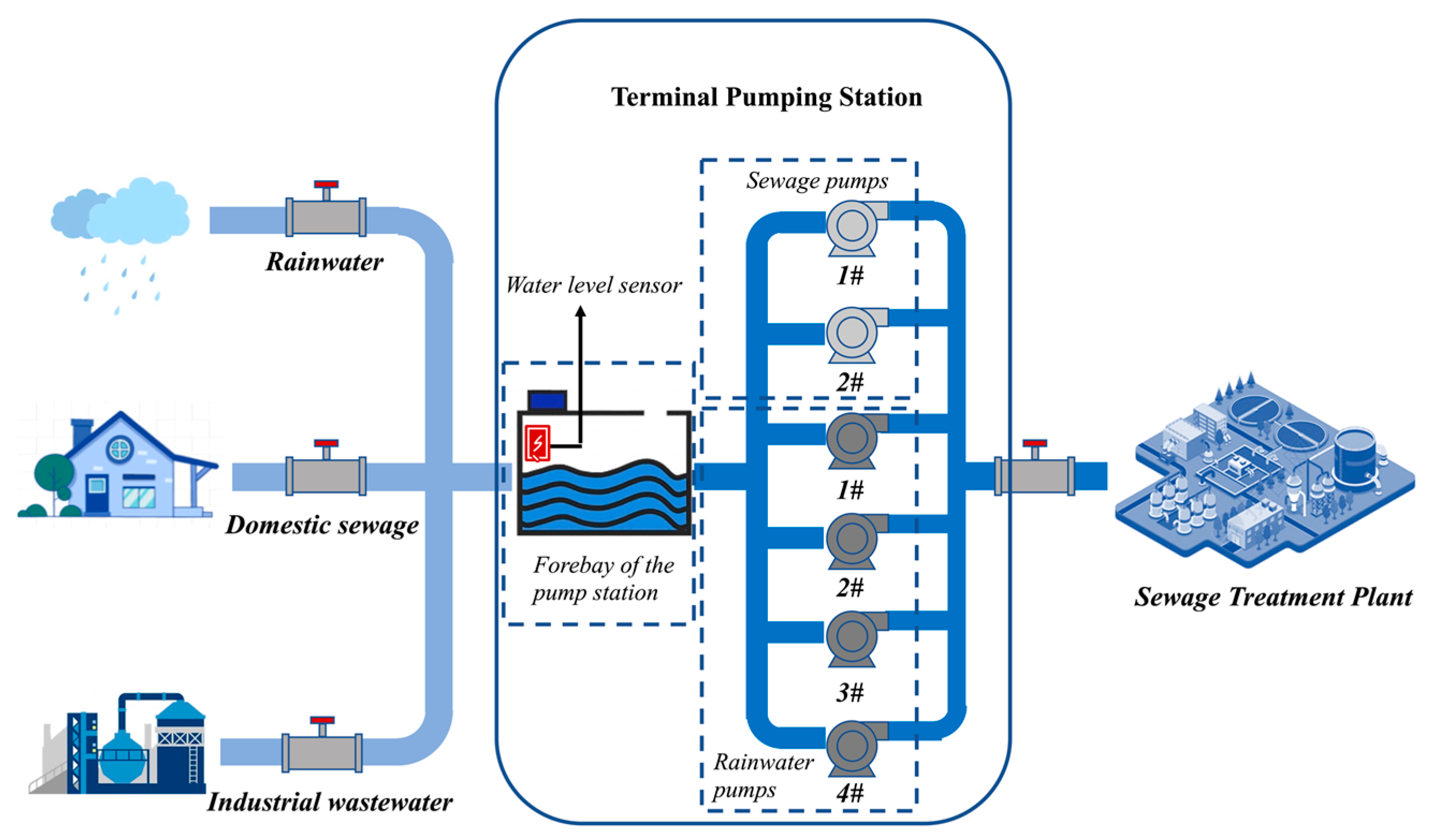
The research area is located in Huangpu District, Shanghai, China, and the schematic of the drainage system in this area is shown in Figure 4. This is a combined drainage system, covering a total area of 1.7 . The total length of the drainage system pipe network is about 55 , with 4067 pipes, 3808 inspection wells, and 1 terminal pumping station. The rainwater drainage capacity of the system is 12 , and the sewage interception capacity is 1.251 . On sunny days, the forebay of the pumping station receives domestic sewage and industrial wastewater in the city. When the water level of the forebay reaches a certain height, the sewage pumps will be turned on to transport the sewage in the forebay to the sewage treatment plant. On rainy days, the forebay also receives rainwater. Affected by the intensity of rainfall, the water level of the forebay tends to rise rapidly. At this time, the sewage pumps and an appropriate number of rainwater pumps will be turned on to quickly transport the sewage to the sewage treatment plant, to prevent the forebay from being flooded.
The data in this research are the forebay water level data of the terminal pumping station of the drainage system. The data spans from 1 January 2020 to 31 December 2020, with a sampling interval of 5 min. The dataset of the forebay water level contains 105,408 observations, and Table 1 shows the characteristics of this dataset with a resolution of 5 min.
In addition, this research also obtained the rainfall data and the number of rainwater pumps and sewage pumps in the same period of time, and the data collection interval is also 5 min.
3.2. Data Normalization
In this research, the interval for the forebay water level data of the pumping station is [−7.382, 6.452], the interval for the rainfall data is [0, 152.4], the interval for the number of rainwater pumps is [0, 4], and the interval for the number of sewage pumps is [0, 2]. The water level data and rainfall data are continuous, while the data for the number of pumps is discrete. The large difference in the dimensions of these features can impact the performance of the neural network and slow down its convergence, significantly affecting the training speed of the model.
The data normalization method used in this research is the MinMaxScaler [46], as shown in Equation (12):
where, is the normalized data; is the original data in the dataset; is the minimum value in the dataset; is the maximum value in the dataset; and are the maximum and minimum expected scaling values, respectively.
In this research, is set to 1 and is set to 0, so that each feature of the sample is linearly mapped to [0, 1].
3.3. Sample Processing
As mentioned earlier, the raw data cannot be directly used to train a neural network model, so the sliding window scheme is employed to establish the relationship between input and output, allowing it to be used for training the neural network model. This research also uses the sliding window scheme for sample processing, sliding the window by one time step at a time until all the data has been processed, in order to create supervised learning samples [47].
Firstly, the length of the output window was set according to the actual usage. Secondly, after determining the output window length, it was found through testing that an input window length that was either too long or too short would reduce the model’s ability to repair data. Therefore, for different data and models, a reasonable sliding window length should be set based on actual usage. The following are the specific sliding window settings in this research.
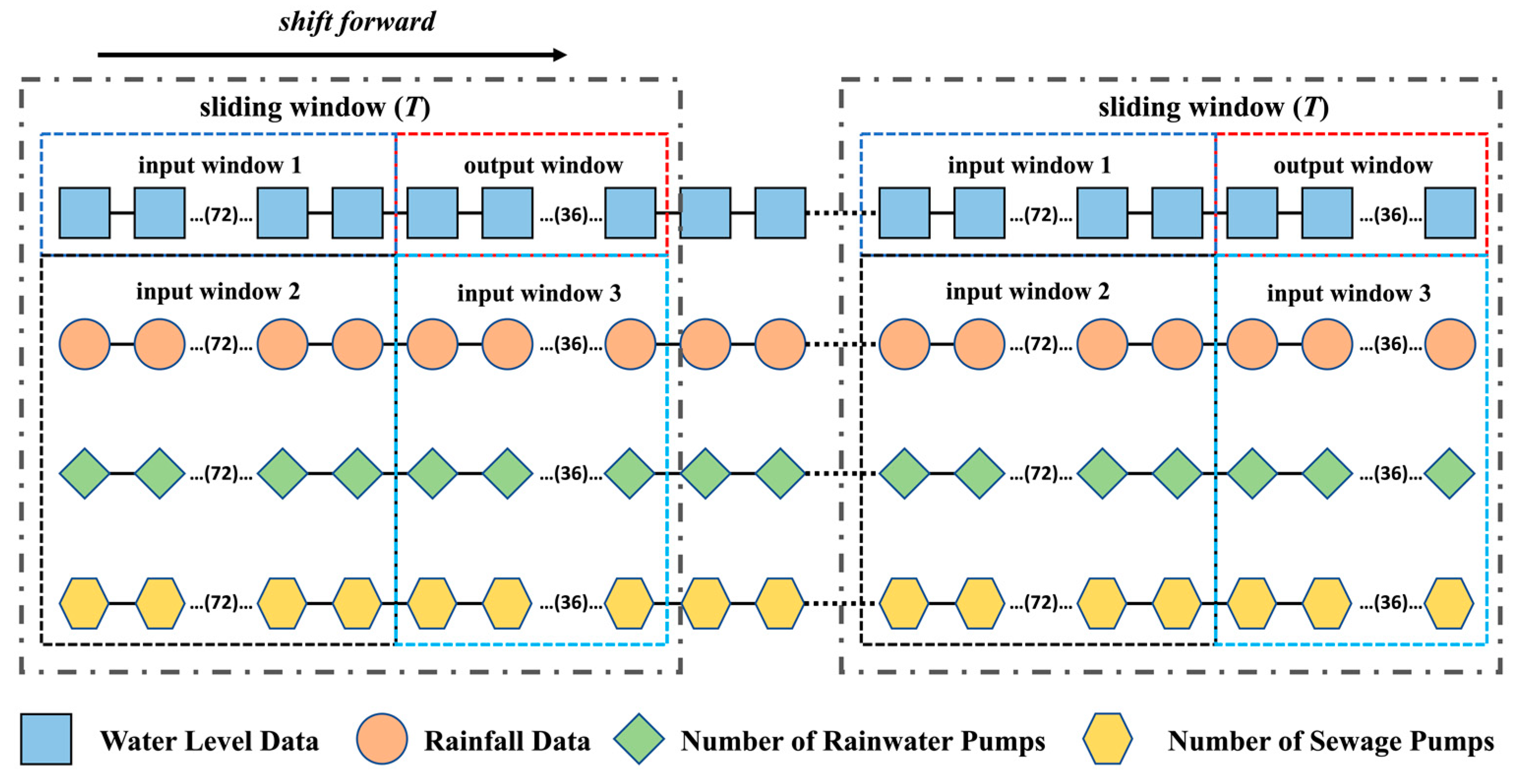
As illustrated in Figure 5, the sliding window in this research has a length of 108, corresponding to 9 h of monitoring data. The sliding window is divided into input window 1, input window 2, input window 3, and output window. By moving forward in time steps of 5 min, the sliding window divides the time series data into input and output combinations of length 108. By applying this process to the data from 1 January 2020 to 17 August 2020, a total of 66,133 training samples can be obtained. In each sample, input window 1 and input window 2 both have a length of 72, containing the water level data for 6 h before the repaired period and the rainfall data, as well as the number of rainwater pumps and sewage pumps, for 6 h before the repaired period, respectively. Input window 3 has a length of 36 and contains the rainfall data, as well as the number of rainwater pumps and sewage pumps, for the repaired period. The output window has a length of 36 and contains the repaired water level data for a 3 h period. The same approach is used to process the test dataset samples.
3.4. Model Development
A deep learning model (Con-GRU) based on one-dimension convolution (Conv1D) and gated recurrent unit (GRU) is proposed in this research, to learn the mapping relationship between the input and output of the training samples in Section 3.3. The Con-GRU model combines the strengths of both models by using the Conv1D layers to extract local features from the input data, and the GRU layer to capture temporal dependencies between these features. This allows the model to better capture complex patterns and dependencies in time series data, while avoiding the limitations of each model when used alone. The Con-GRU model is designed with the architecture to handle different types of data. The deep learning architecture that combines Conv1D and GRU has been successfully applied in the field of water supply research [11,48], demonstrating the effectiveness of this type of structure. In the case of optimizing the neural network structure and parameter configuration, the effectiveness of Con-GRU in the water level data repair process is guaranteed.
3.4.1. Con-GRU Model Design
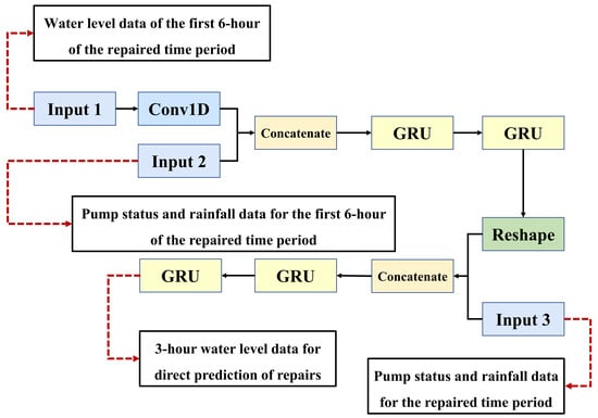
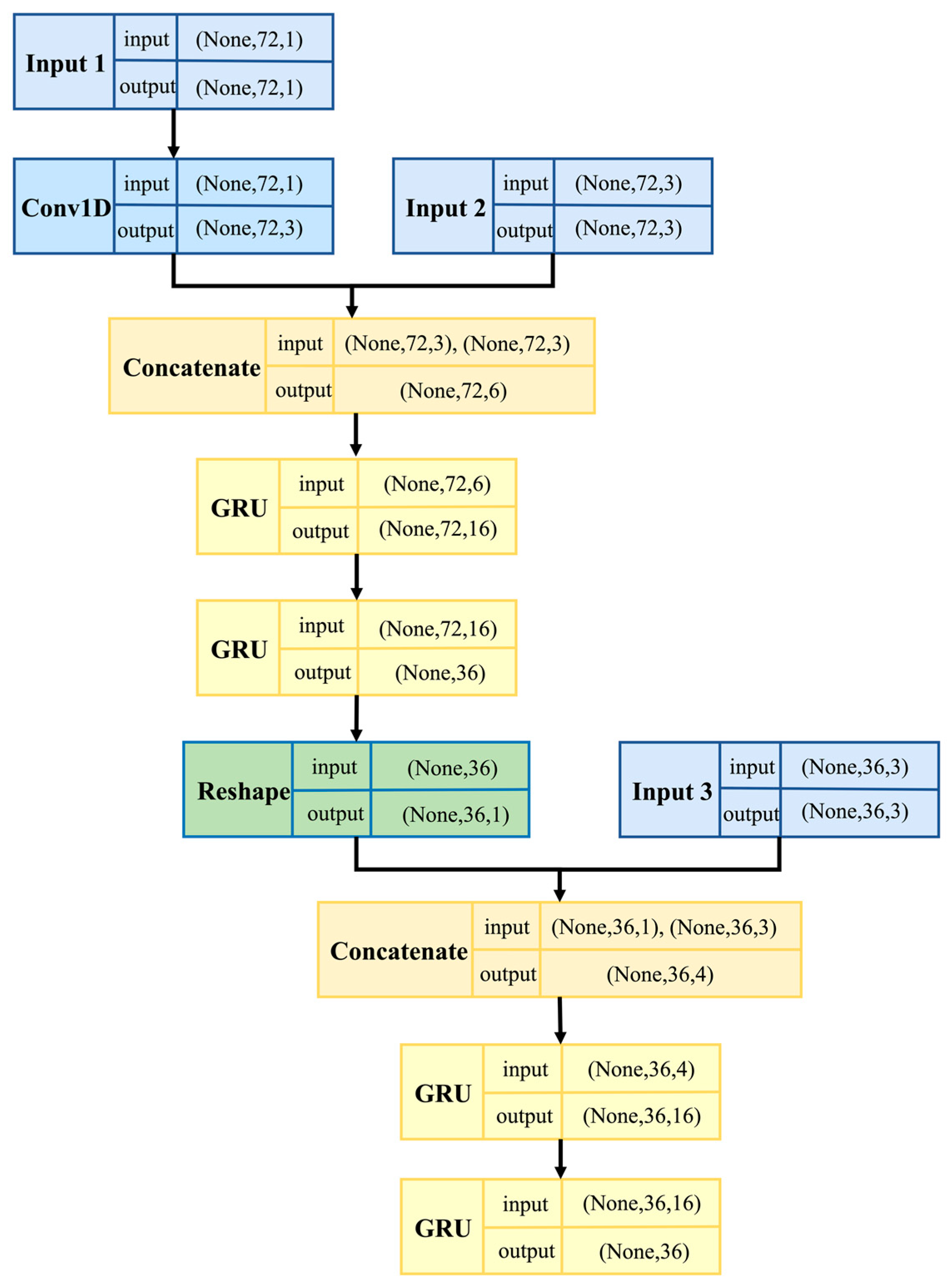
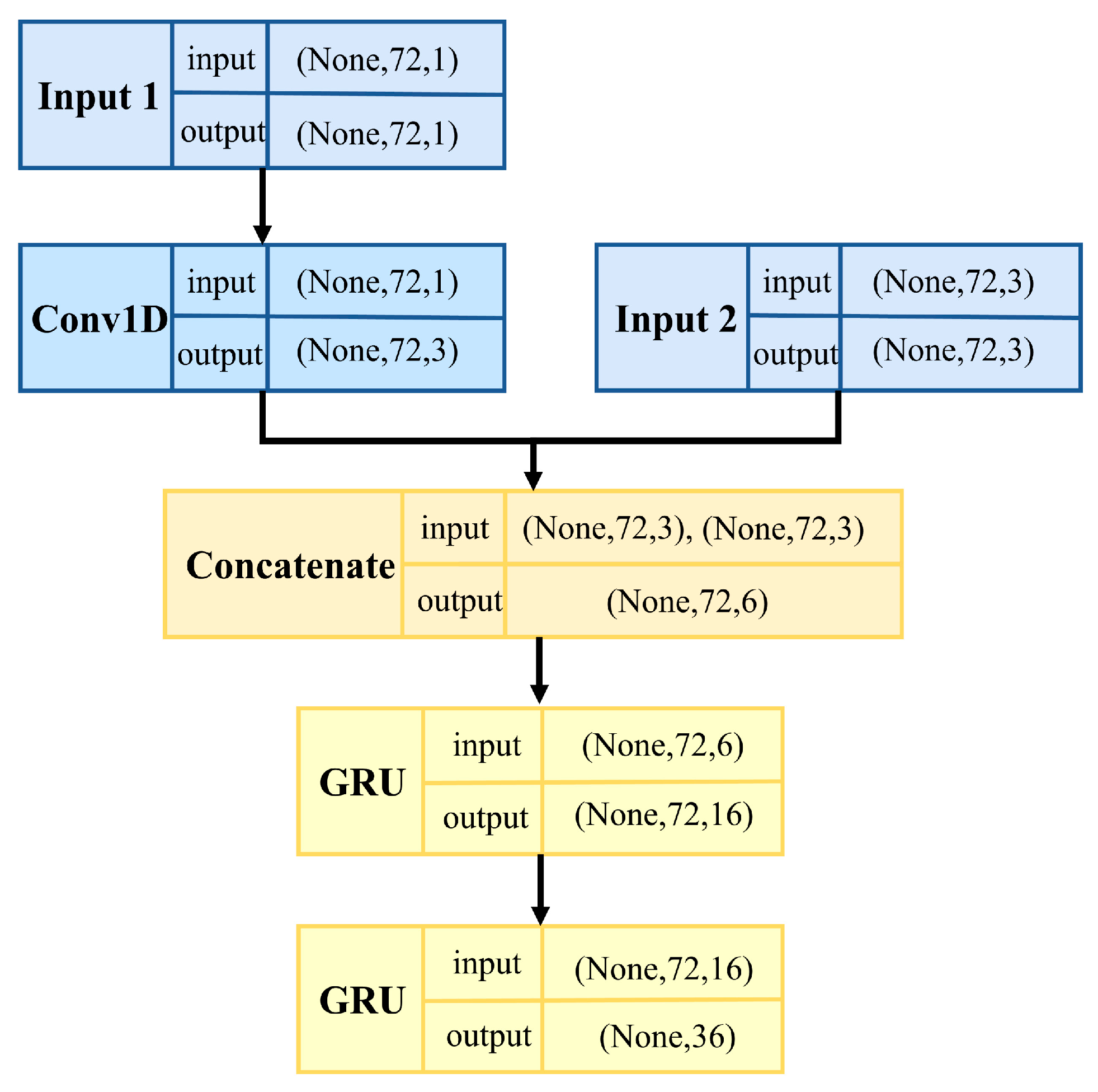
This research focuses on the repair of the water level data of the pumping station forebay. Deep learning is used to build a multistep prediction model of the water level data, which ensures the rationality of the monitoring data, and lays a data foundation for further use of the repaired data to build the hydraulic model. The Con-GRU model is shown in Figure 6.
Figure 6 not only illustrates the structure of the Con-GRU model, but also shows the data shape of the input and output for each layer of the model. It can be seen that the Con-GRU model has three input layers, corresponding to the data from input window 1, input window 2, and input window 3, as described in Section 3.3.
The input layer 1 receives the water level data for 6 h prior to the period to be repaired, and performs feature extraction using Conv1D with a convolution kernel length of 6 (extracting features for continuous half-hour water level data). The input layer 2 receives the rainfall data, as well as the number of rainwater pumps and sewage pumps, for 6 h prior to the period to be repaired, and combines these with the features extracted by Conv1D. Two layers of GRU, with 16 and 36 neurons, are then used to obtain the time relationship between the water level data, rainfall, number of rainwater pumps, and number of sewage pumps, in order to preliminarily predict the water level data within 3 h. The input layer 3 receives the rainfall data, number of rainwater pumps, and number of sewage pumps within 3 h during the period to be repaired, and fuses these with the preliminary water level prediction results from the above GRU layers. Finally, two layers of GRU, with 16 and 36 neurons, are used to extract time-dependent features of the fused features, resulting in the final prediction of the water level data for a 3 h period.
The reason for using the rainfall data, the number of rainwater pumps, and the number of sewage pumps within 3 h during the period to be repaired is that the water level data is affected by the above three data, and the Con-GRU model can obtain the control characteristics of the above three data for the water level. Therefore, in the process of repairing water level data, the preliminary water level value can be further regulated by using the three kinds of data, which can effectively calibrate the water level data information under real rainfall and switch pump status.
Since the Con-GRU model is based on the repair of water level monitoring data, it is best to propose more applicable deep learning models based on the DSMDR framework, according to the specific drainage monitoring data type.
3.4.2. Hyperparameter Configuration
The effectiveness of a prediction model is not only determined by its design, but also by the configuration of its hyperparameters. By setting the hyperparameters properly, the model is able to capture the underlying characteristics of the data and produce accurate forecasts. The Con-GRU model has four hyperparameters that need to be configured: (1) the size of the Conv1D window, cw; (2) the dimension of the output space of the first GRU layer, gd; (3) the learning rate of the model, lr; and (4) the batch size for training, bs.
To determine the optimal configuration of the hyperparameters, a combination of grid search and cross-validation methods are employed in this research [49]. Grid search is a method for exhaustively searching the space of possible hyperparameter combinations by specifying a range of values for each hyperparameter. The grid search algorithm evaluates the performance of the model for each combination of hyperparameter values within the specified range, using cross-validation to determine the average score for each combination. The combination with the highest average score is selected as the optimal choice, and the trained model is returned. By specifying the search range for each hyperparameter, grid search can be used to identify the optimal combination of hyperparameter values for a given model. In addition, this research sets appropriate ranges of hyperparameter variations based on existing research [48,50], which laid the foundation for finding the optimal hyperparameter configuration.
Table 2 presents the search range and the optimal configuration for the hyperparameters of the Con-GRU model. In addition to the hyperparameter configuration, 15% of the data in the training dataset is reserved for use as a validation dataset. This validation dataset is used to evaluate the performance of the model during training. The model is trained for a set number of epochs (in this case, 10) and the loss on the validation dataset is computed. If the loss on the validation dataset improves, the model’s parameters are saved. This process is repeated until the model has completed the specified number of training epochs. By evaluating the model on a validation dataset, we can ensure that the model is not overfitting to the training data, and is generalizing well to unseen data.
4. Results and Discussion
In this research, the data from 1 January 2020 to 17 August 2020 are used as the training and validation datasets, while the data from 18 August 2020 to 31 December 2020 are used as the test dataset. To evaluate the effectiveness of the Con-GRU model in repairing the water level data of the forebay, the performance of the LSTM and ANN models are also compared. The hyperparameters of the LSTM and ANN models are also optimized using the method described in Section 3.4.2. The performance of the models on the validation dataset is evaluated in Section 4.1, which only considers the repair of the 3 h data. In Section 4.2, the performance of the models on the validation dataset is also evaluated, but the repair of the water level data is assumed to be performed on a daily basis. After the models repair the first 3 h of data, the predicted repair values are used as the new inputs for the models to repair the second 3 h of data, and this process is repeated until the data for one day is repaired. In Section 4.3, the performance of the models on the test dataset is evaluated using the approach described in Section 4.2. Section 4.4 evaluates the impact of pump status and rainfall on the performance of the Con-GRU model in repairing the data.
4.1. Performance of 3 h Data Repair Results on the Validation Dataset
For the evaluation of the repaired 3 h data, the inputs to the models consist of actual monitoring data. One hundred samples were randomly selected from the validation dataset for evaluation, and Table 3 shows the average values of the models’ direct repair results indicators for the 3 h water level data in the above samples. It can be seen from the results that all three models have a repair effect on the 3 h level data, but the Con-GRU model significantly outperforms the other two models in terms of all the three prediction indicators (e.g., average NSE 0.8136). The Con-GRU model also performs best when considering model complexity. The two deep learning models (Con-GRU and LSTM) are significantly better than the ANN model, which also shows that the deep learning model has more obvious advantages in the repair of drainage monitoring data.
Furthermore, to further analyze the generalization ability of the models, the error distributions of the three indicators are depicted in Figure 7. It can be observed that the Con-GRU model has a better generalization ability compared to the other two models, as indicated by the tight boxes in the box plots. The NSE indicator for most of the samples for the three models is above 0.5, indicating that the models have a certain level of stability in repairing the water level data.
4.2. Performance of 1 Day Data Iteratively Repaired Results on the Validation Dataset
This section involves an iterative process in which the models use the repaired 3 h water level data as new input, making predictions and repairs until the data for a full day is successfully repaired.
Figure 8 shows the changes in the forebay water level of the pumping station on the validation dataset for 4 days, representing four different change modes. The change of the data on 6 March 2020 has a significant periodicity. In the case of using the real data from 18:00–23:55 on 5 March 2020, the subsequent water level data are all from the iterative repair of the models. It can be seen that if the data on 6 March is abnormal throughout the day, the models can still achieve perfect data repair. The data repair effect of the Con-GRU model is better than that of the ANN and LSTM models. The MAE, RMSE, and NSE of the Con-GRU model’s iteratively repaired data on 6 March are 0.3710, 0.4854, and 0.8820, respectively. The indicators of Con-GRU are better than the ANN model (0.4595, 0.6273, and 0.8028) and the LSTM model (0.5795, 0.7015, and 0.7535). It can still be seen from Figure 8 that the data repair effect of Con-GRU in other scenarios is also better than that of the ANN and LSTM models. The Con-GRU model has demonstrated an ability to accurately predict water levels based on rainfall data and pump status, suggesting that it has learned the relationship between these factors and water levels. This capability allows the model to effectively handle data repair scenarios in various conditions.
4.3. Performance of 1 Day Data Iteratively Repaired Results on the Test Dataset
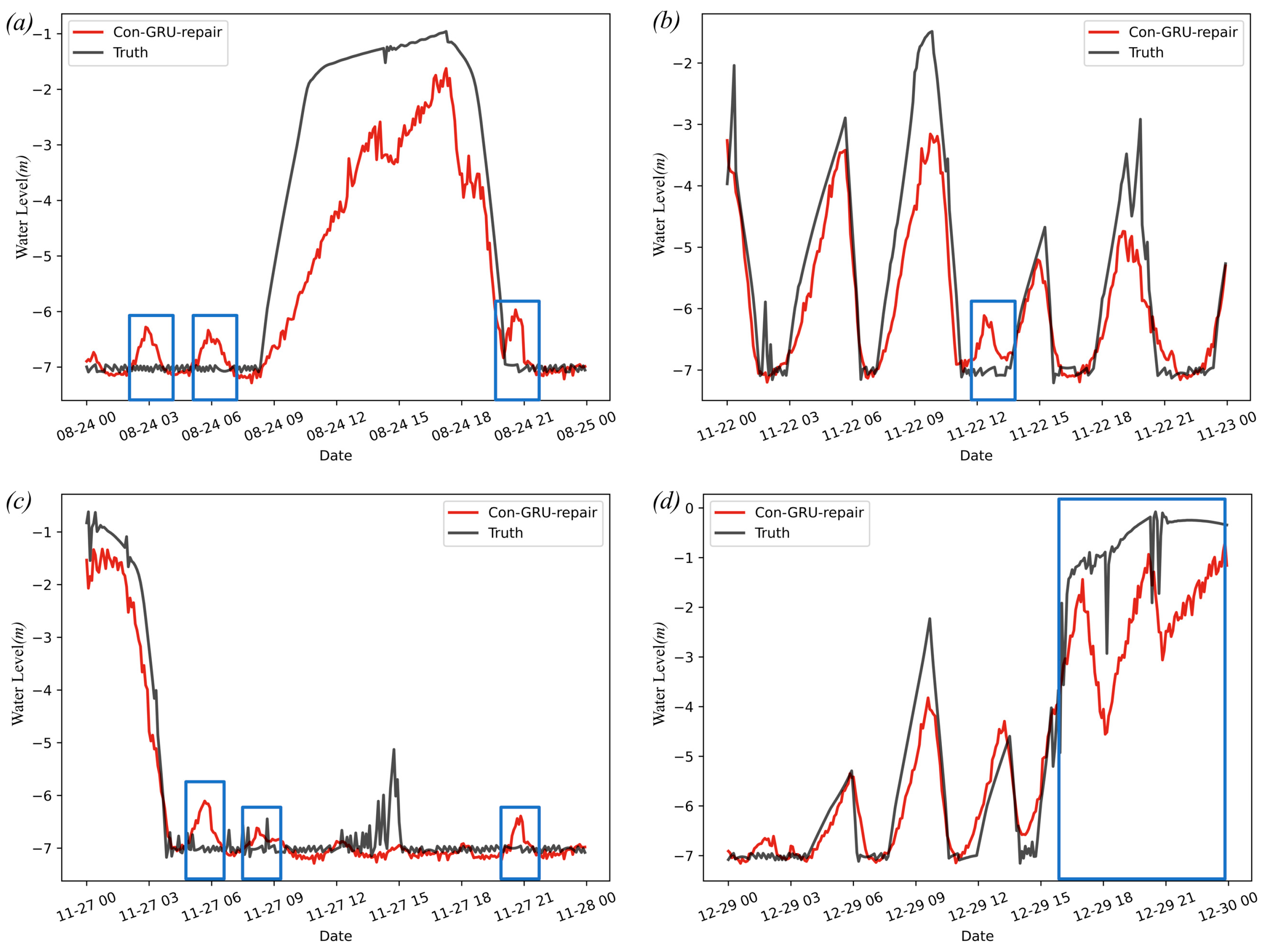
In Section 4.2, although the iterative prediction strategy is adopted by the Con-GRU model for data repair, the repaired data is still in the validation dataset. In order to further verify the effectiveness of the model for repairing water level data, the test dataset from 18 August 2020 to 31 December 2020 was evaluated in this case. As in Section 4.2, the four-day data with different change characteristics in the test dataset is first selected. Under the same assumption that the data of the day is abnormal, the Con-GRU model is used in iterative repair. The repair results are shown in Figure 9.
As an example, the Con-GRU model’s repair effect on the water level data for 24 August 2020 is generally consistent with the actual water level change, with MAE, RMSE, and NSE values of 0.7107, 1.0474, and 0.8409, respectively. However, the repaired data shown in the framed section of Figure 9a exhibits a different change pattern from the actual monitoring data for the time periods of 01:30–04:00, 05:00–07:00, and 20:00–21:00. Upon analysis of the pump operating conditions during these times, it was found that the only running sewage pump was turned off at 00:55, and remained off until 03:05. Under these circumstances, the forebay water level should have risen, but the actual level was recorded at approximately −7 m, which is not consistent with the pump being off. It is believed that this discrepancy was caused by abnormal data transmission. The Con-GRU model’s repaired data more accurately reflects the pump switching conditions in this time period, resulting in a water level change that is more consistent with the actual situation.
Similarly, such properties also exist in Figure 9b–d, where the NSE of the three cases are 0.8174, 0.9573, and 0.7981, respectively. Further analysis of the difference between the repaired data and the real monitoring data in Figure 9d shows that in the real situation, a sewage pump was turned on at 17:10 and lasted until 17:50. The real monitoring data did not reflect the drop of the water level, but the repaired data of the Con-GRU model can perfectly reflect it. The repaired water level data dropped from −2.096 m to −4.098 m during 17:10–17:50, which is in line with the characteristics of the water level change in the opened pump state. After that, from 18:20 to 20:15, the previously opened sewage pump was turned off under real conditions, and during this period, it was in the rainfall stage. The water level in the repaired data also increased from −4.065 m to −1.099 m, which was more consistent with the change mode compared with the real water level data. Then, from 20:20 to 20:50, another sewage pump was turned on according to the real scheduling situation, and the repaired water level data also dropped from −1.555 m to −3.061 m. Finally, in the real situation, the pump was closed, and the repaired water level data continued to rise on the basis of −3.061 m.
The above analysis demonstrates that the Con-GRU model is capable of effectively repairing abnormal water level data over extended periods of time, and producing repaired data that is more consistent with the pump status and rainfall conditions. This reflects the model’s strong robustness and adaptability to complex scenarios.
4.4. Influence of Pump Status and Rainfall on Repair Effect
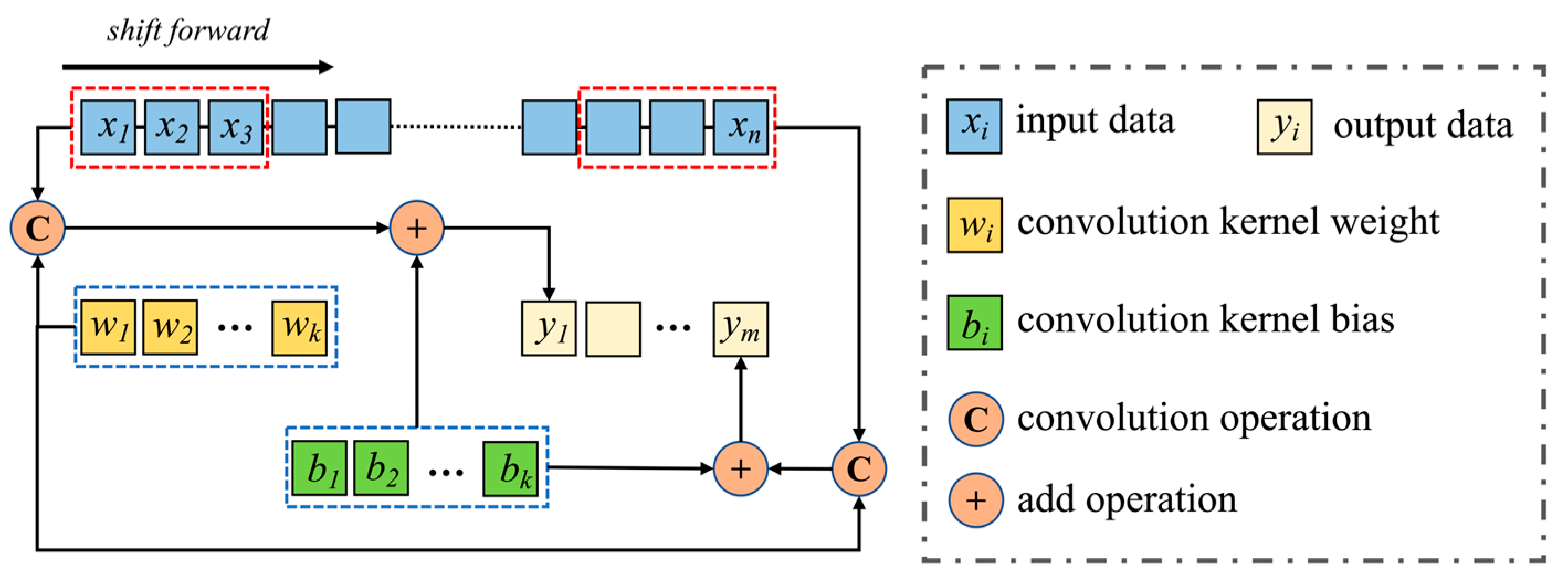
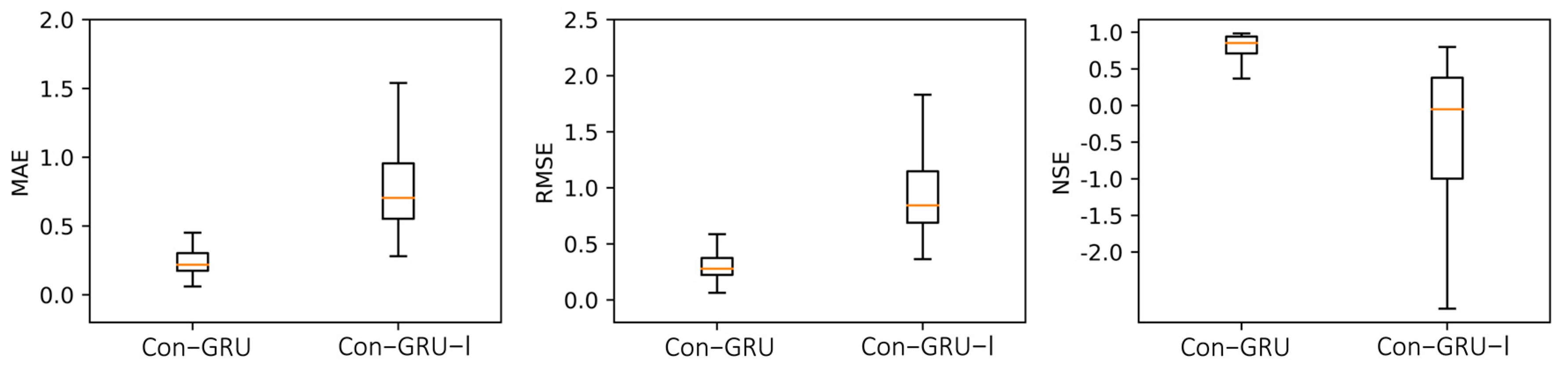
The Con-GRU model differs from traditional prediction models in that it incorporates both rainfall data and pump status from the corresponding period into the repair of the 3 h water level data, effectively using “future information” to improve the accuracy of the repair process. This section presents the Con-GRU-I model, the structure of which is illustrated in Figure 10. In contrast to the Con-GRU model, the Con-GRU-I model eliminates the input module for “future information” (i.e., input 3), allowing for an evaluation of the impact of input 3 on the data repair effect.
To compare the effectiveness of the Con-GRU model and the Con-GRU-I model in repairing 3 h data, 100 samples were randomly selected from the validation dataset for evaluation, as demonstrated in Figure 11. This follows the same procedure described in Section 4.1. The results show that the Con-GRU model generally performs better in terms of data repair compared to the Con-GRU-I model. Specifically, the inclusion of input 3 leads to an increase in the average values of the MAE, RMSE, and NSE indicators, from 0.8657, 1.0375, and −0.5495, to 0.2566, 0.3206, and 0.8025, respectively. This indicates that the rainfall data and pump status from the repaired period contribute to the improvement of the forebay water level data repair.
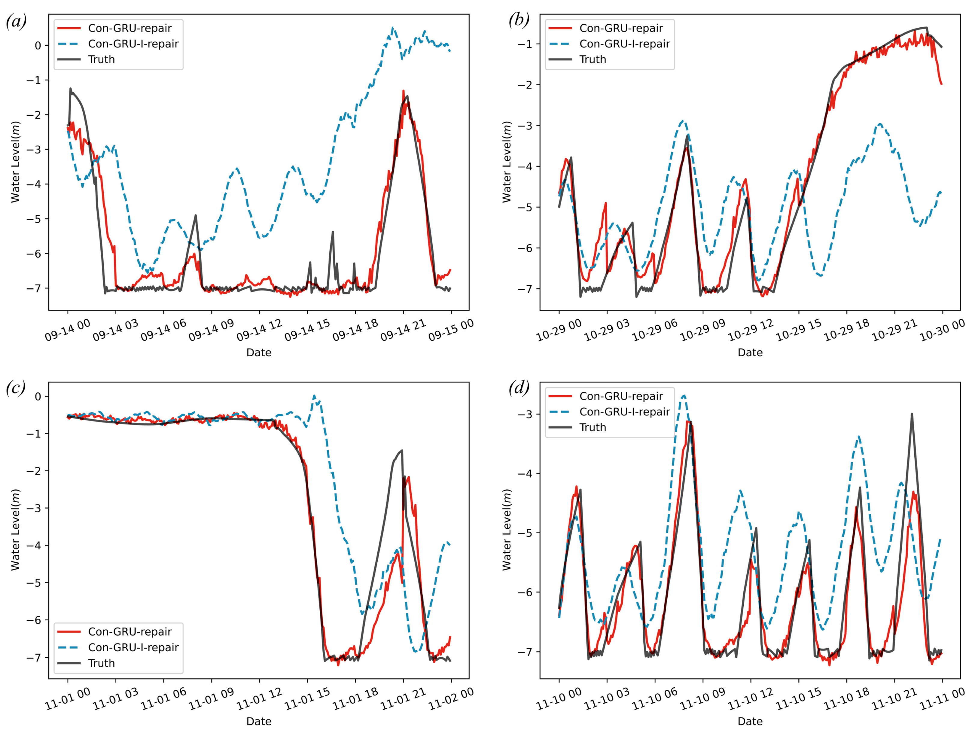
In this section, two models were used to iteratively repair water level data on the test dataset in order to assess the repair effectiveness of the models when the water level data was abnormal for one consecutive day. The Con-GRU model achieved the optimal MAE, RMSE, and NSE values of 0.0810, 0.0659, and 0.9703, respectively, while the Con-GRU-I model only achieved values of 0.1419, 0.1169, and 0.6025, respectively. Figure 12 compares the results of the two models in iteratively repairing one-day water level data. The results show that the Con-GRU model is significantly superior to the Con-GRU-I model in terms of repairing long-term water level data.
Figure 12a–d shows that the NSE indicators of the Con-GRU model are 0.8940, 0.9703, 0.9133, and 0.8722, respectively. The Con-GRU-I model can be broadly classified into three cases for iterative repair of data. Firstly, as shown in Figure 12a, the Con-GRU-I model is unable to effectively predict the change in real water level data within a day, resulting in a large difference between the repaired data change pattern and the actual water level change pattern. Secondly, as shown in Figure 12b, the Con-GRU-I model is able to capture the change pattern of the real water level data in the first half of the repair, but loses this ability in the second half. Within the time period of 00:00–15:00, the MAE value can reach 1.0476, while the MAE value for 15:00–24:00 is only 3.1867. Similarly, in Figure 12c, the MAE value for the Con-GRU-I model can reach 0.1438 in the time period of 00:00–12:00, while the NSE value for 12:00–24:00 is only 2.5543. One cause of the degradation of the performance of the Con-GRU-I model is the accumulation of errors due to iterative prediction, which leads to distorted results when attempting to repair the model. Additionally, the inclusion of rainfall data and pump status in the input to the model helps to correct for changes in the water level data, whereas the Con-GRU-I model lacks this information when attempting to repair the data. Thirdly, as shown in Figure 12d, when the water level data exhibits a periodic change pattern, the Con-GRU-I model is able to capture it. However, the Con-GRU-I model still performs worse than the Con-GRU model in terms of repairing the daily water level data, with an MAE and RMSE of only 1.1386 and 0.9560, respectively. In summary, the inclusion of rainfall data and pump status during the repair period has a significant impact on the repair of the forebay water level data. It not only helps the repair model capture the true change pattern of the data, but also helps to alleviate the accumulation of errors due to iterative prediction, thereby improving the accuracy and authenticity of the repaired data.
5. Conclusions
This research proposes a deep learning-based approach to drainage monitoring data repair, and evaluates it using pumping station forebay water level data. The proposed Con-GRU deep learning model for repairing forebay water level data in drainage systems outperforms the traditional ANN and LSTM models. By treating data repair as a predictive procedure, the Con-GRU model effectively utilizes “future information” such as rainfall data and pump status for the targeted time period, capturing the patterns of change in forebay water level data and improving the accuracy of the repair.
The DSMDR framework covers all the steps of using deep learning methods for drainage system monitoring data repair, providing a direction for the establishment of different methods under this framework. The forebay water level monitoring data repaired by the Con-GRU model is more consistent with the real switching pump status and rainfall conditions of the drainage system, making it more reliable for water modeling processes.
However, other factors such as holidays and temperature also affect changes in the forebay water levels, which may be addressed by incorporating additional input variables that are explanatory of the prediction results. Future research can explore the integration of these factors, and further improve the accuracy and applicability of the proposed framework. Overall, this research provides valuable insights into the development of effective and comprehensive methods for long-term abnormal data repair in drainage system monitoring data.
Author Contributions
Conceptualization, L.H., S.J. and L.C.; methodology, L.H.; software, L.H., C.S. and L.C.; validation, L.H., K.X. and J.N.; formal analysis, L.H., Z.C. and C.S.; investigation, J.N. and L.C.; resources, S.J.; data curation, S.J., Z.C. and L.C.; writing—original draft preparation, L.H.; writing—review and editing, L.H., K.X. and L.C.; visualization, L.H.; supervision, S.J., J.N. and L.C.; project administration, S.J. All authors have read and agreed to the published version of the manuscript.
Funding
This research received no external funding.
Institutional Review Board Statement
Not applicable.
Informed Consent Statement
Not applicable.
Data Availability Statement
Data available on request due to restrictions, e.g., privacy. The data presented in this study are available from the Shanghai Urban Construction Design and Research Institute (SUCDRI) authors.
Acknowledgments
We would like to express our gratitude to the Shanghai Urban Construction Design Research Institute for their support in providing data, and to the Smart Water Joint Innovation R&D Center of Tongji University for providing computational support.
Conflicts of Interest
The authors declare no conflict of interest.
References
- Eggimann, S.; Mutzner, L.; Wani, O.; Schneider, M.Y.; Spuhler, D.; Matthew, M.; Beutler, P.; Maurer, M. The Potential of Knowing More: A Review of Data-Driven Urban Water Management. Environ. Sci. Technol. 2017, 51, 2538–2553. [Google Scholar] [CrossRef] [PubMed]
- Zhang, A.; Song, S.; Wang, J.; Yu, P.S. Time series data cleaning: From anomaly detection to anomaly repairing. Proc. VLDB Endow. 2017, 10, 1046–1057. [Google Scholar] [CrossRef]
- Boubiche, D.E.; Pathan, A.K.; Lloret, J.; Zhou, H.; Hong, S.; Amin, S.O.; Feki, M.A. Advanced industrial wireless sensor networks and intelligent IoT. IEEE Commun. Mag. 2018, 56, 14–15. [Google Scholar] [CrossRef]
- Xu, Y.; Sun, Y.; Wan, J.; Liu, X.; Song, Z. Industrial big data for fault diagnosis: Taxonomy, review, and applications. IEEE Access 2017, 5, 17368–17380. [Google Scholar] [CrossRef]
- Su, X.; Shao, G.; Vause, J.; Tang, L. An integrated system for urban environmental monitoring and management based on the environmental internet of things. Int. J. Sustain. Dev. World Ecol. 2013, 20, 205–209. [Google Scholar] [CrossRef]
- Hill, D.J.; Minsker, B.S. Anomaly detection in streaming environmental sensor data: A data-driven modeling approach. Environ. Model. Softw. 2010, 25, 1014–1022. [Google Scholar] [CrossRef]
- Khani, M.J.; Shirmohammadi, Z. SRCM: An Efficient Method for Energy Consumption Reduction in Wireless Body Area Networks based on Data Similarity. Adhoc Sens. Wirel. Netw. 2022, 51, 173–187. [Google Scholar]
- Zhang, W.; Tan, G.; Ding, N. Traffic Information Detection Based on Scattered Sensor Data: Model and Algorithms. Adhoc Sens. Wirel. Netw. 2013, 18, 225–240. [Google Scholar]
- Čampulová, M.; Michálek, J.; Mikuška, P.; Bokal, D. Nonparametric algorithm for identification of outliers in environmental data. J. Chemom. 2018, 32, e2997. [Google Scholar] [CrossRef]
- Holešovský, J.; Čampulová, M.; Michálek, J. Semiparametric outlier detection in nonstationary times series: Case study for atmospheric pollution in Brno, Czech Republic. Atmos. Pollut. Res. 2018, 9, 27–36. [Google Scholar] [CrossRef]
- Chen, L.; Yan, H.; Yan, J.; Wang, J.; Tao, T.; Xin, K.; Li, S.; Pu, Z.; Qiu, J. Short-term water demand forecast based on automatic feature extraction by one-dimensional convolution. J. Hydrol. 2022, 606, 127440. [Google Scholar] [CrossRef]
- Akouemo, H.N.; Povinelli, R.J. Data improving in time series using ARX and ANN models. IEEE Trans. Power Syst. 2017, 32, 3352–3359. [Google Scholar] [CrossRef]
- Fauconnier, C.; Haesbroeck, G. Outliers detection with the minimum covariance determinant estimator in practice. Stat. Methodol. 2009, 6, 363–379. [Google Scholar] [CrossRef]
- Cai, L.; Thornhill, N.F.; Kuenzel, S.; Pal, B.C. Real-time detection of power system disturbances based on k-nearest neighbor analysis. IEEE Access 2017, 5, 5631–5639. [Google Scholar] [CrossRef]
- An, Q.; Tao, Z.; Xu, X.; El Mansori, M.; Chen, M. A data-driven model for milling tool remaining useful life prediction with convolutional and stacked LSTM network. Measurement 2020, 154, 107461. [Google Scholar] [CrossRef]
- Roberts, C.; Nair, M. Arbitrary discrete sequence anomaly detection with zero boundary LSTM. arXiv 2018, arXiv:1803.02395. [Google Scholar]
- Tariq, S.; Lee, S.; Shin, Y.; Lee, M.S.; Jung, O.; Chung, D.; Woo, S.S. Detecting anomalies in space using multivariate convolutional LSTM with mixtures of probabilistic PCA. In Proceedings of the 25th ACM SIGKDD International Conference on Knowledge Discovery & Data Mining, Anchorage, AK, USA, 4–8 August 2019; Association for Computing Machinery: New York, NY, USA, 2019; pp. 2123–2133. [Google Scholar]
- Su, Y.; Zhao, Y.; Niu, C.; Liu, R.; Sun, W.; Pei, D. Robust anomaly detection for multivariate time series through stochastic recurrent neural network. In Proceedings of the 25th ACM SIGKDD International Conference on Knowledge Discovery & Data Mining, Anchorage, AK, USA, 4–8 August 2019; Association for Computing Machinery: New York, NY, USA, 2019; pp. 2828–2837. [Google Scholar]
- Tan, F.H.S.; Park, J.R.; Jung, K.; Lee, J.S.; Kang, D. Cascade of one class classifiers for water level anomaly detection. Electronics 2020, 9, 1012. [Google Scholar] [CrossRef]
- Ye, F.; Liu, Z.; Liu, Q.; Wang, Z. Hydrologic time series anomaly detection based on flink. Math. Probl. Eng. 2020, 2020, 3187697. [Google Scholar] [CrossRef]
- Shao, P.; Ye, F.; Liu, Z.; Wang, X.; Lu, M.; Mao, Y. Improving iForest for Hydrological Time Series Anomaly Detection; Springer: Berlin/Heidelberg, Germany, 2020; pp. 170–183. [Google Scholar]
- Sun, J.; Lou, Y.; Ye, F. Research on anomaly pattern detection in hydrological time series. In Proceedings of the 2017 14th Web Information Systems and Applications Conference (WISA), Liuzhou, China, 11–12 November 2017; pp. 38–43. [Google Scholar]
- Xu, C.; Wang, J.; Hu, M.; Wang, W. A new method for interpolation of missing air quality data at monitor stations. Environ. Int. 2022, 169, 107538. [Google Scholar] [CrossRef]
- Wang, P.; Zhang, T.; Zheng, Y.; Hu, T. A multi-view bidirectional spatiotemporal graph network for urban traffic flow imputation. Int. J. Geogr. Inf. Sci. 2022, 36, 1231–1257. [Google Scholar] [CrossRef]
- Park, S.; Jung, S.; Jung, S.; Rho, S.; Hwang, E. Sliding window-based LightGBM model for electric load forecasting using anomaly repair. J. Supercomput. 2021, 77, 12857–12878. [Google Scholar] [CrossRef]
- Wang, M.; Kumar, S.S.; Cheng, J.C. Automated sewer pipe defect tracking in CCTV videos based on defect detection and metric learning. Autom. Constr. 2021, 121, 103438. [Google Scholar] [CrossRef]
- Guo, Z.; Leitão, J.P.; Simões, N.E.; Moosavi, V. Data-driven flood emulation: Speeding up urban flood predictions by deep convolutional neural networks. J. Flood Risk Manag. 2021, 14, e12684. [Google Scholar] [CrossRef]
- Mullapudi, A.; Lewis, M.J.; Gruden, C.L.; Kerkez, B. Deep reinforcement learning for the real time control of stormwater systems. Adv. Water Resour. 2020, 140, 103600. [Google Scholar] [CrossRef]
- Chen, K.; Wang, H.; Valverde-Pérez, B.; Zhai, S.; Vezzaro, L.; Wang, A. Optimal control towards sustainable wastewater treatment plants based on multi-agent reinforcement learning. Chemosphere 2021, 279, 130498. [Google Scholar] [CrossRef]
- Kratzert, F.; Herrnegger, M.; Klotz, D.; Hochreiter, S.; Klambauer, G. NeuralHydrology–interpreting LSTMs in hydrology. In Explainable AI: Interpreting, Explaining and Visualizing Deep Learning; Springer: Berlin/Heidelberg, Germany, 2019; pp. 347–362. [Google Scholar]
- Lees, T.; Reece, S.; Kratzert, F.; Klotz, D.; Gauch, M.; De Bruijn, J.; Kumar Sahu, R.; Greve, P.; Slater, M.; Dadson, S.J. Hydrological concept formation inside long short-term memory (LSTM) networks. Hydrol. Earth Syst. Sci. 2022, 26, 3079–3101. [Google Scholar] [CrossRef]
- Frame, J.M.; Kratzert, F.; Klotz, D.; Gauch, M.; Shelev, G.; Gilon, O.; Qualls, L.M.; Gupta, H.V.; Nearing, G.S. Deep learning rainfall–runoff predictions of extreme events. Hydrol. Earth Syst. Sci. 2022, 26, 3377–3392. [Google Scholar] [CrossRef]
- Klotz, D.; Kratzert, F.; Gauch, M.; Keefe Sampson, A.; Brandstetter, J.; Klambauer, G.; Hochreiter, S.; Nearing, G. Uncertainty estimation with deep learning for rainfall–runoff modeling. Hydrol. Earth Syst. Sci. 2022, 26, 1673–1693. [Google Scholar] [CrossRef]
- Song, W.; Gao, C.; Zhao, Y.; Zhao, Y. A time series data filling method based on LSTM—Taking the stem moisture as an example. Sensors 2020, 20, 5045. [Google Scholar] [CrossRef]
- Ren, H.; Cromwell, E.; Kravitz, B.; Chen, X. Using deep learning to fill spatio-temporal data gaps in hydrological monitoring networks. Hydrol. Earth Syst. Sci. Discuss. 2019, 1–20. [Google Scholar] [CrossRef]
- Kulanuwat, L.; Chantrapornchai, C.; Maleewong, M.; Wongchaisuwat, P.; Wimala, S.; Sarinnapakorn, K.; Boonya-aroonnet, S. Anomaly detection using a sliding window technique and data imputation with machine learning for hydrological time series. Water 2021, 13, 1862. [Google Scholar] [CrossRef]
- Yang, J.; Li, J. Application of deep convolution neural network. In Proceedings of the 2017 14th International Computer Conference on Wavelet Active Media Technology and Information Processing (ICCWAMTIP), Chengdu, China, 15–17 December 2017; pp. 229–232. [Google Scholar]
- LeCun, Y.; Boser, B.; Denker, J.; Henderson, D.; Howard, R.; Hubbard, W.; Jackel, L. Handwritten digit recognition with a back-propagation network. In Advances in Neural Information Processing Systems 2; Morgan Kaufmann: Burlington, MA, USA, 1989; Volume 2. [Google Scholar]
- Bouvrie, J. Notes on Convolutional Neural Networks. 2006. Available online: http://web.mit.edu/jvb/www/papers/cnn_tutorial.pdf (accessed on 3 November 2022).
- Cheng, H.; Xie, Z.; Shi, Y.; Xiong, N. Multi-step data prediction in wireless sensor networks based on one-dimensional CNN and bidirectional LSTM. IEEE Access 2019, 7, 117883–117896. [Google Scholar] [CrossRef]
- Teng, S.; Chen, G.; Liu, Z.; Cheng, L.; Sun, X. Multi-sensor and decision-level fusion-based structural damage detection using a one-dimensional convolutional neural network. Sensors 2021, 21, 3950. [Google Scholar] [CrossRef]
- Hochreiter, S.; Schmidhuber, J. Long short-term memory. Neural Comput. 1997, 9, 1735–1780. [Google Scholar] [CrossRef]
- Cho, K.; Van Merriënboer, B.; Bahdanau, D.; Bengio, Y. On the properties of neural machine translation: Encoder-decoder approaches. arXiv 2014, arXiv:1409.1259. [Google Scholar]
- Bandara, K.; Bergmeir, C.; Smyl, S. Forecasting across time series databases using recurrent neural networks on groups of similar series: A clustering approach. Expert Syst. Appl. 2020, 140, 112896. [Google Scholar] [CrossRef]
- Zhang, D.; Hølland, E.S.; Lindholm, G.; Ratnaweera, H. Hydraulic modeling and deep learning based flow forecasting for optimizing inter catchment wastewater transfer. J. Hydrol. 2018, 567, 792–802. [Google Scholar] [CrossRef]
- Hossein Javaheri, S. Response Modeling in Direct Marketing: A Data Mining Based Approach for Target Selection. 2008. Available online: https://www.diva-portal.org/smash/record.jsf?pid=diva2%3A1024362&dswid=3350 (accessed on 15 November 2022).
- Smyl, S. Forecasting Short Time Series with LSTM Neural Networks. 2016. Available online: https://gallery.azure.ai/Tutorial/Forecasting-Short-Time-Series-with-LSTM-Neural-Networks-2 (accessed on 5 January 2023).
- Pu, Z.; Yan, J.; Chen, L.; Li, Z.; Tian, W.; Tao, T.; Xin, K. A hybrid Wavelet-CNN-LSTM deep learning model for short-term urban water demand forecasting. Front. Environ. Sci. Eng. 2023, 17, 22. [Google Scholar] [CrossRef]
- Bergstra, J.; Bengio, Y. Random search for hyper-parameter optimization. J. Mach. Learn. Res. 2012, 13, 281–305. [Google Scholar]
- Guo, G.; Liu, S.; Wu, Y.; Li, J.; Zhou, R.; Zhu, X. Short-term water demand forecast based on deep learning method. J. Water Resour. Plan. Manag. 2018, 144, 04018076. [Google Scholar] [CrossRef]
Figure 1.
The process framework of drainage system monitoring data repair.

Figure 2.
One-dimensional convolution operation.

Figure 3.
The calculation process of GRU: (a) calculation of reset gate; (b) calculation of update gate; (c) calculation of candidate hidden state; (d) calculation of hidden state.
Figure 3.
The calculation process of GRU: (a) calculation of reset gate; (b) calculation of update gate; (c) calculation of candidate hidden state; (d) calculation of hidden state.

Figure 4.
The schematic of the drainage system in Huangpu District.

Figure 5.
The sample processing process of the research data.

Figure 6.
The structure of the Con-GRU model.

Figure 7.
Comparison of three models on the validation dataset for 3 h data repair results.

Figure 8.
Comparison of three models in iterative repair on validation dataset: (a) results of data repair on 6 March 2020; (b) results of data repair on 10 March 2020; (c) results of data repair on 23 April 2020; (d) results of data repair on 18 July 2020.
Figure 8.
Comparison of three models in iterative repair on validation dataset: (a) results of data repair on 6 March 2020; (b) results of data repair on 10 March 2020; (c) results of data repair on 23 April 2020; (d) results of data repair on 18 July 2020.

Figure 9.
Comparison of the Con-GRU model in iterative repair on test dataset: (a) results of data repair on 24 August 2020; (b) results of data repair on 22 November 2020; (c) results of data repair on 27 November 2020; (d) results of data repair on 29 December 2020.
Figure 9.
Comparison of the Con-GRU model in iterative repair on test dataset: (a) results of data repair on 24 August 2020; (b) results of data repair on 22 November 2020; (c) results of data repair on 27 November 2020; (d) results of data repair on 29 December 2020.

Figure 10.
The structure of the Con-GRU-I model.

Figure 11.
Comparison of the Con-GRU model and Con-GRU-I model on the validation dataset for 3 h data repair results.
Figure 11.
Comparison of the Con-GRU model and Con-GRU-I model on the validation dataset for 3 h data repair results.

Figure 12.
Comparison of the Con-GRU model and Con-GRU-I model in iterative repair on test dataset: (a) results of data repair on 14 September 2020; (b) results of data repair on 29 October 2020; (c) results of data repair on 1 November 2020; (d) results of data repair on 10 November 2020.
Figure 12.
Comparison of the Con-GRU model and Con-GRU-I model in iterative repair on test dataset: (a) results of data repair on 14 September 2020; (b) results of data repair on 29 October 2020; (c) results of data repair on 1 November 2020; (d) results of data repair on 10 November 2020.


Table 1.
The descriptive statistics of the forebay water level data.
| Mean Level (m) | Maximum (m) | Minimum (m) | Standard Deviation | Skewness | Kurtosis |
|---|---|---|---|---|---|
| −5.502 | 6.452 | −7.382 | 2.187 | 1.586 | 2.051 |
Table 2.
The hyperparameter search range and optimal configuration of the Con-GRU model.
| Hyperparameter | Search Range | Optimal Configuration |
|---|---|---|
| cw | [2, 4, 6, 8, 10, 12] | 6 |
| gd | [10, 12, 14, 16, 18] | 16 |
| lr | ranging from 0.0005 to 0.04 with an increase of 0.0005 | 0.001 |
| bs | [256, 512, 1024, 2048] | 1024 |
Table 3.
Average indicators values of three models from 100 samples.
| Model | MAE (m) | RMSE (m) | NSE | AIC | BIC |
|---|---|---|---|---|---|
| ANN | 0.3981 | 0.4827 | 0.7791 | 221,622.3 | 510,494.1 |
| LSTM | 0.4168 | 0.5045 | 0.7613 | 96,271.2 | 221,850.8 |
| Con-GRU | 0.2843 | 0.3558 | 0.8136 | 27,579.3 | 63,772.9 |
Disclaimer/Publisher’s Note: The statements, opinions and data contained in all publications are solely those of the individual author(s) and contributor(s) and not of MDPI and/or the editor(s). MDPI and/or the editor(s) disclaim responsibility for any injury to people or property resulting from any ideas, methods, instructions or products referred to in the content. |
© 2023 by the authors. Licensee MDPI, Basel, Switzerland. This article is an open access article distributed under the terms and conditions of the Creative Commons Attribution (CC BY) license (https://creativecommons.org/licenses/by/4.0/).
Share and Cite
MDPI and ACS Style
He, L.; Ji, S.; Xin, K.; Chen, Z.; Chen, L.; Nan, J.; Song, C. Application of Deep Learning in Drainage Systems Monitoring Data Repair—A Case Study Using Con-GRU Model. Water 2023, 15, 1635. https://doi.org/10.3390/w15081635
AMA Style
He L, Ji S, Xin K, Chen Z, Chen L, Nan J, Song C. Application of Deep Learning in Drainage Systems Monitoring Data Repair—A Case Study Using Con-GRU Model. Water. 2023; 15(8):1635. https://doi.org/10.3390/w15081635
Chicago/Turabian StyleHe, Li, Shasha Ji, Kunlun Xin, Zewei Chen, Lei Chen, Jun Nan, and Chenxi Song. 2023. "Application of Deep Learning in Drainage Systems Monitoring Data Repair—A Case Study Using Con-GRU Model" Water 15, no. 8: 1635. https://doi.org/10.3390/w15081635
Note that from the first issue of 2016, this journal uses article numbers instead of page numbers. See further details here.