
Modeling Fate and Transport of Nutrients and Heavy Metals in the Waters of a Tropical Mexican Lake to Predict Pollution Scenarios
 , and
, and 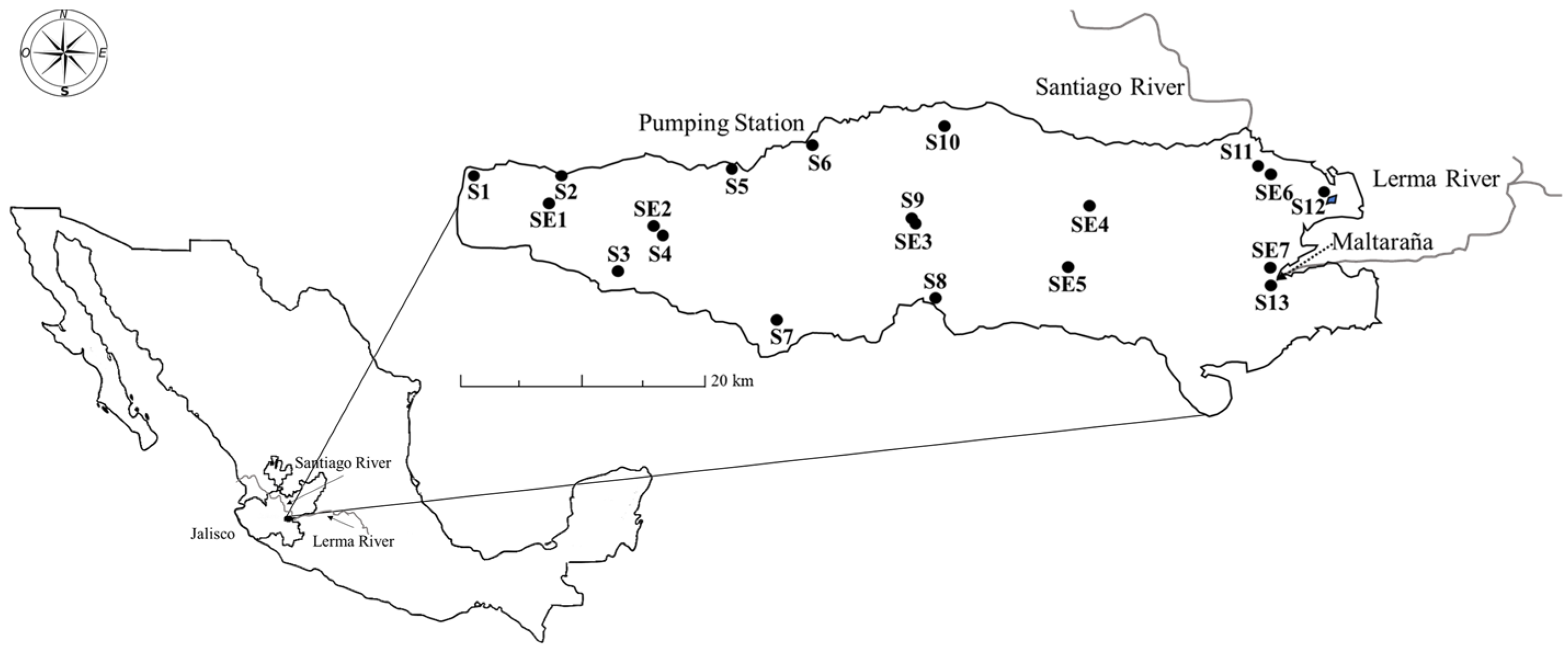
Abstract
:1. Introduction
2. Materials and Methods
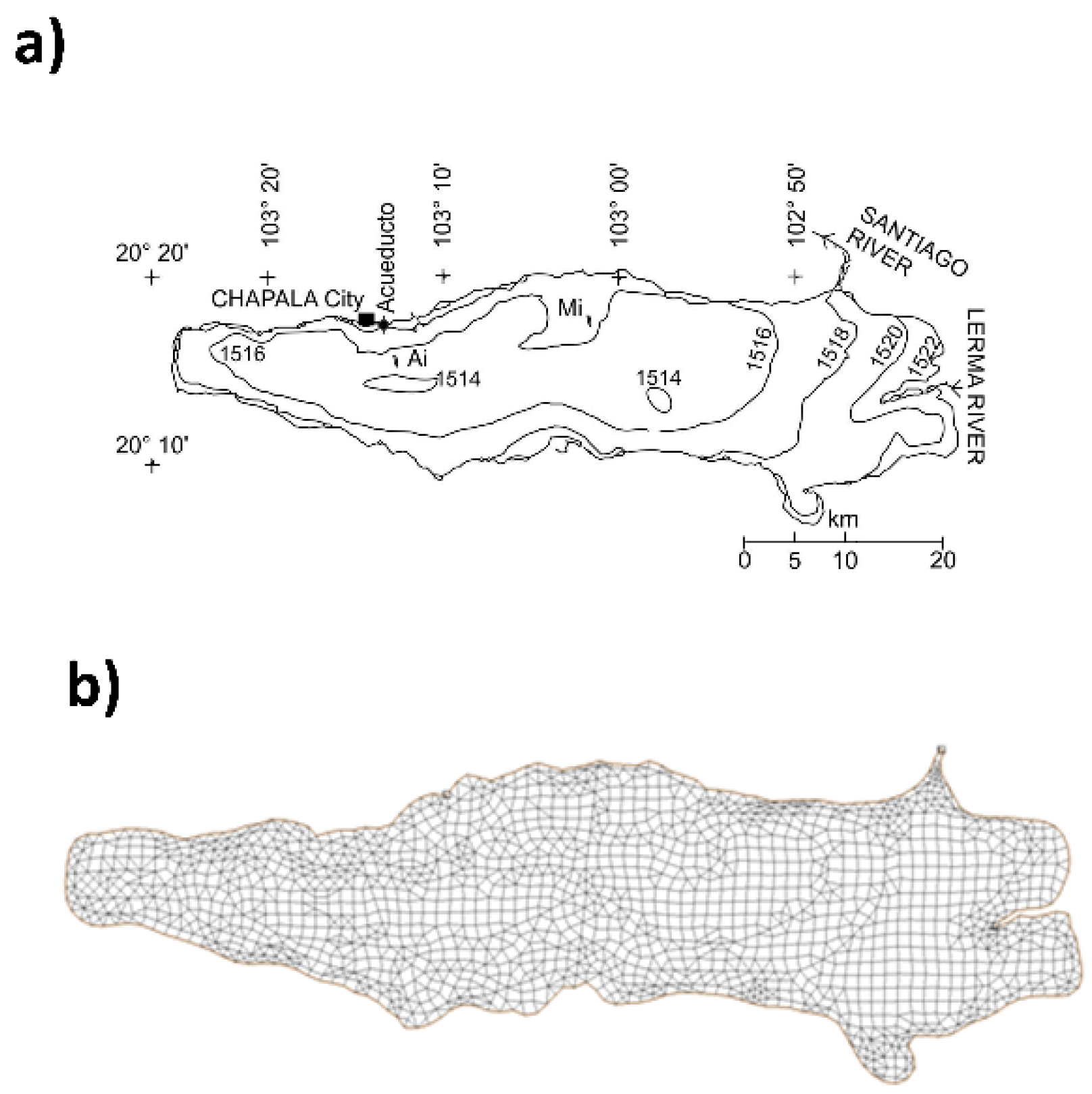
2.1. Study Area
2.2. Water Sampling
2.3. Nutrient Analysis
2.4. Metal Analysis
2.5. Measurement of Hydraulic Parameters
2.6. Fate and Transport Models of Pollutants
2.6.1. Governing Equations
Rate of momentum out of control volume ± Sum of forces acting on control volume
2.6.2. Model Setup
2.7. Model Calibration Procedures
2.8. Model Validation
3. Results and Discussion
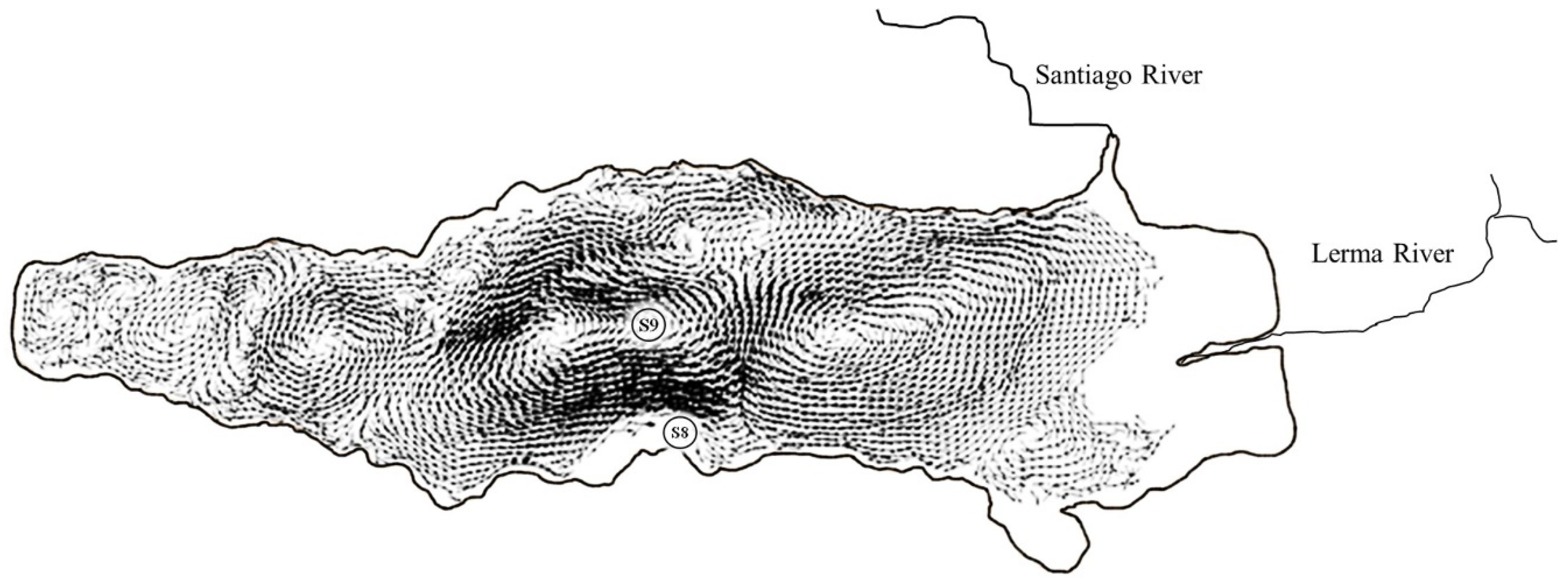
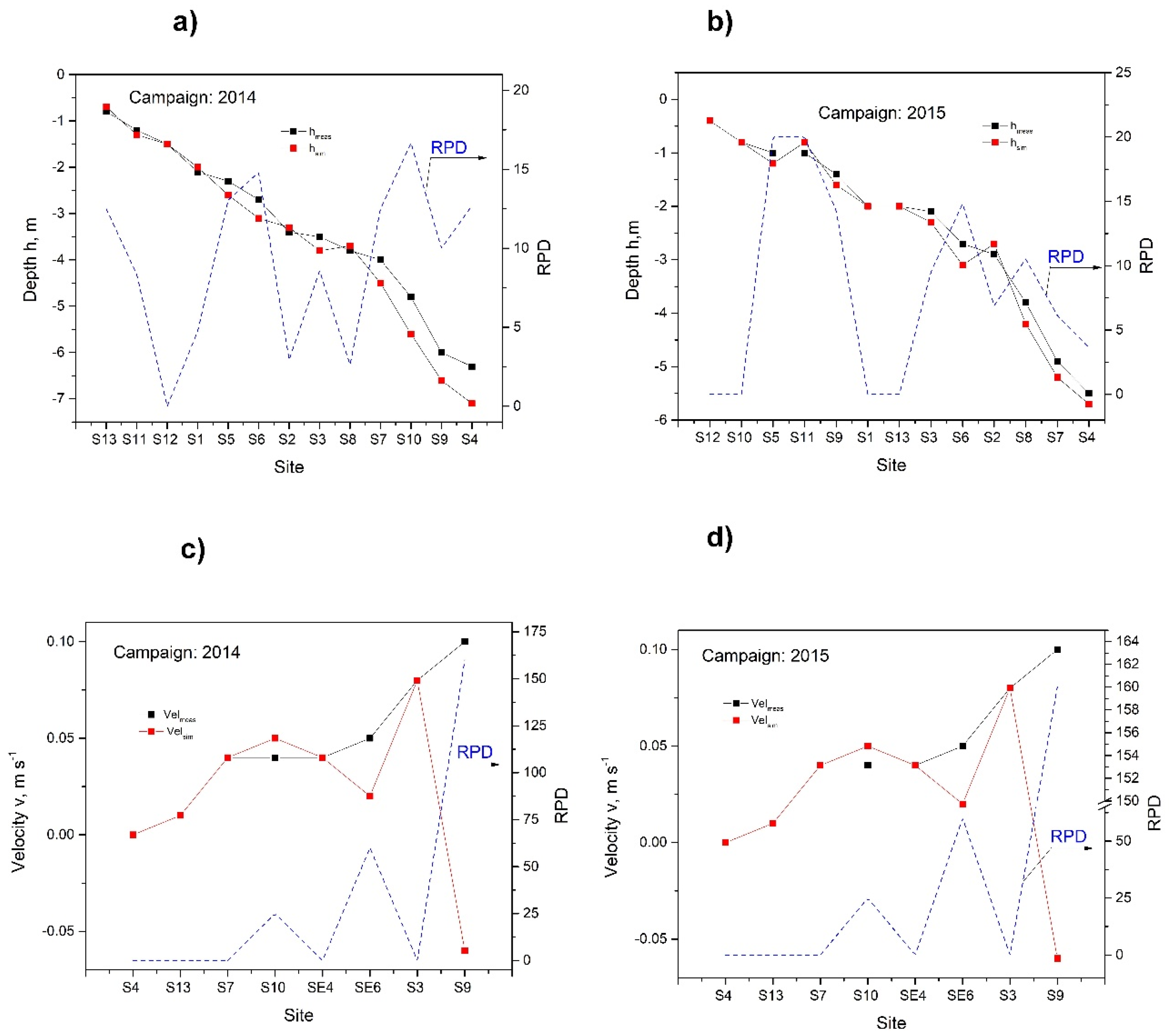
3.1. Hydraulic Model Calibration Results
3.2. Calibration Results of Model Coefficients
3.3. Pollutant Simulations
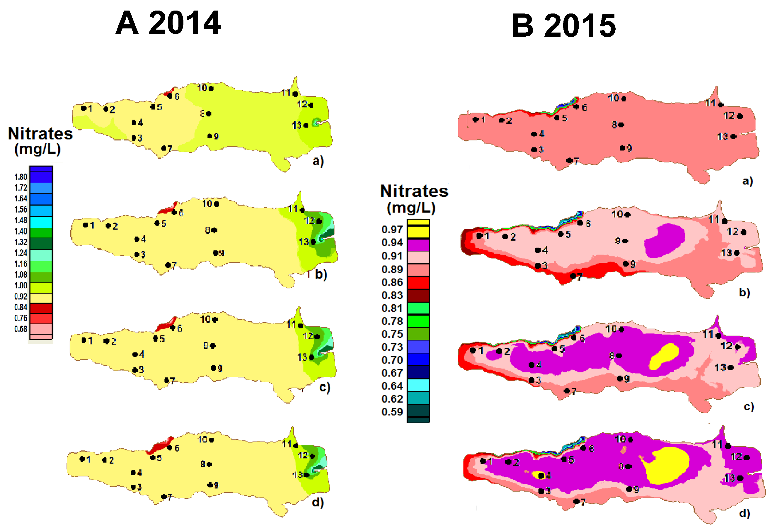
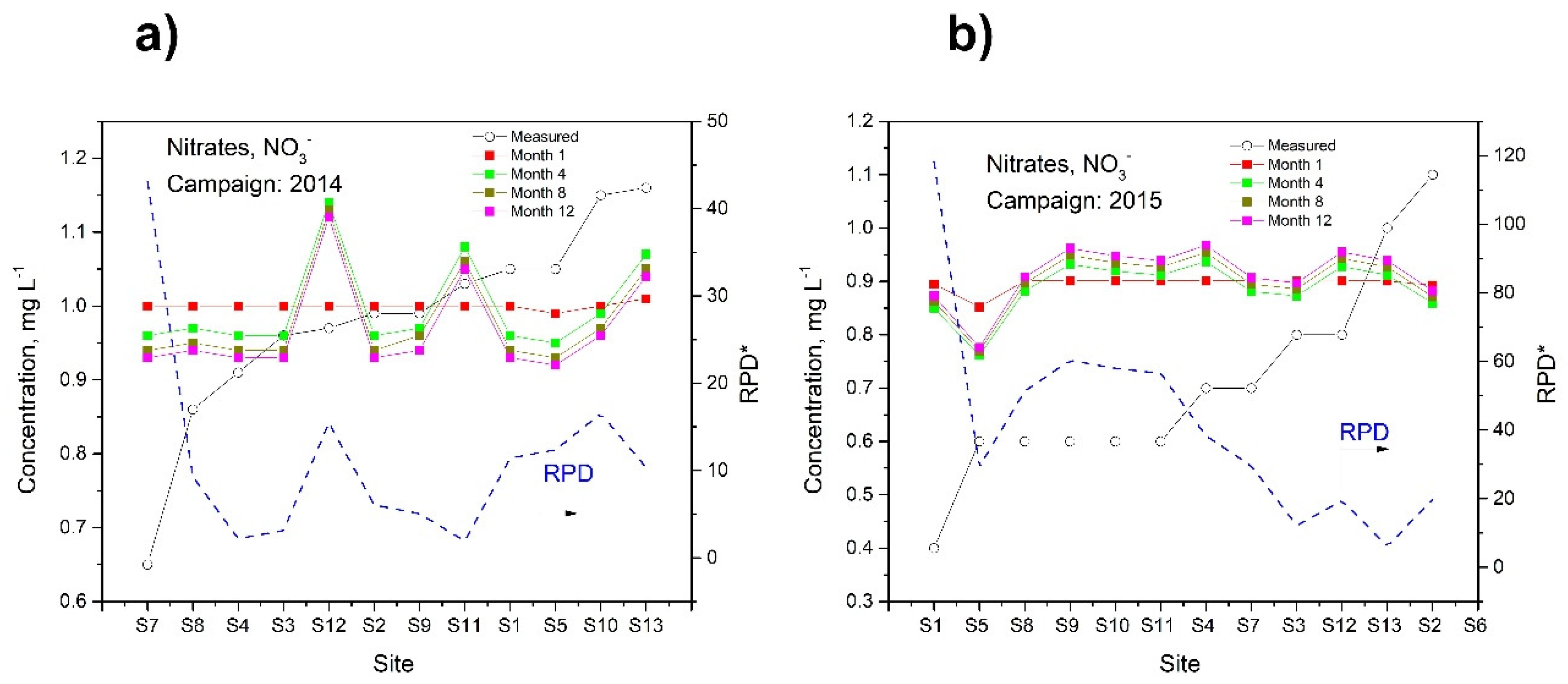
3.3.1. Nitrates
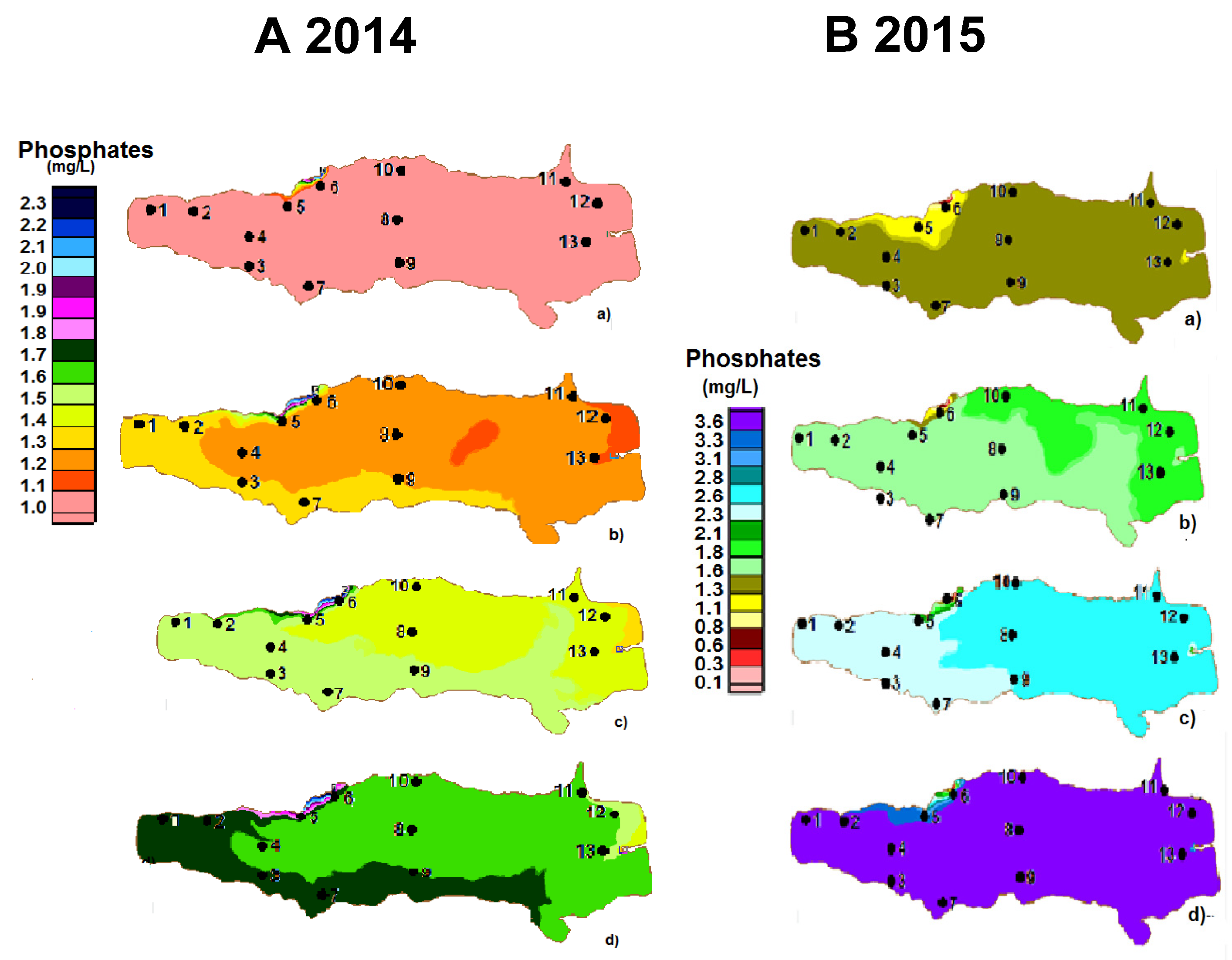
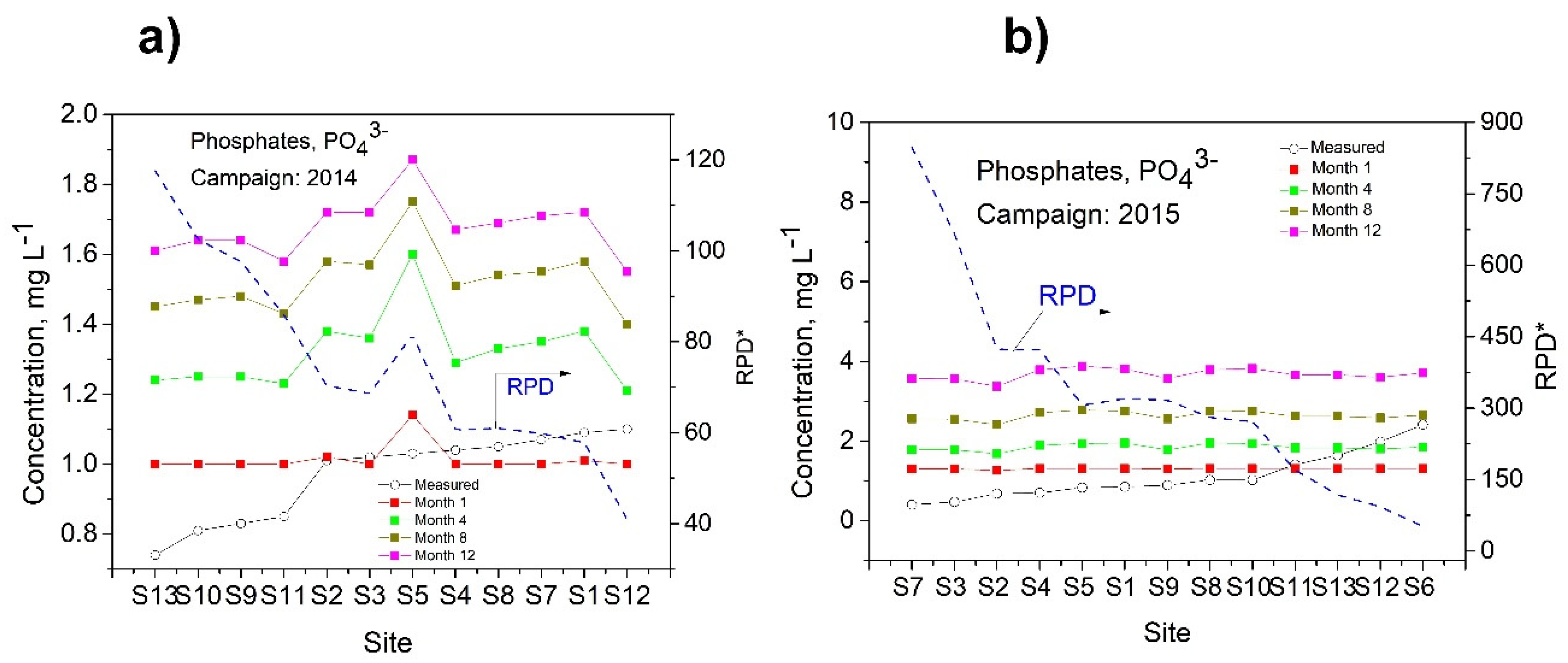
3.3.2. Phosphates
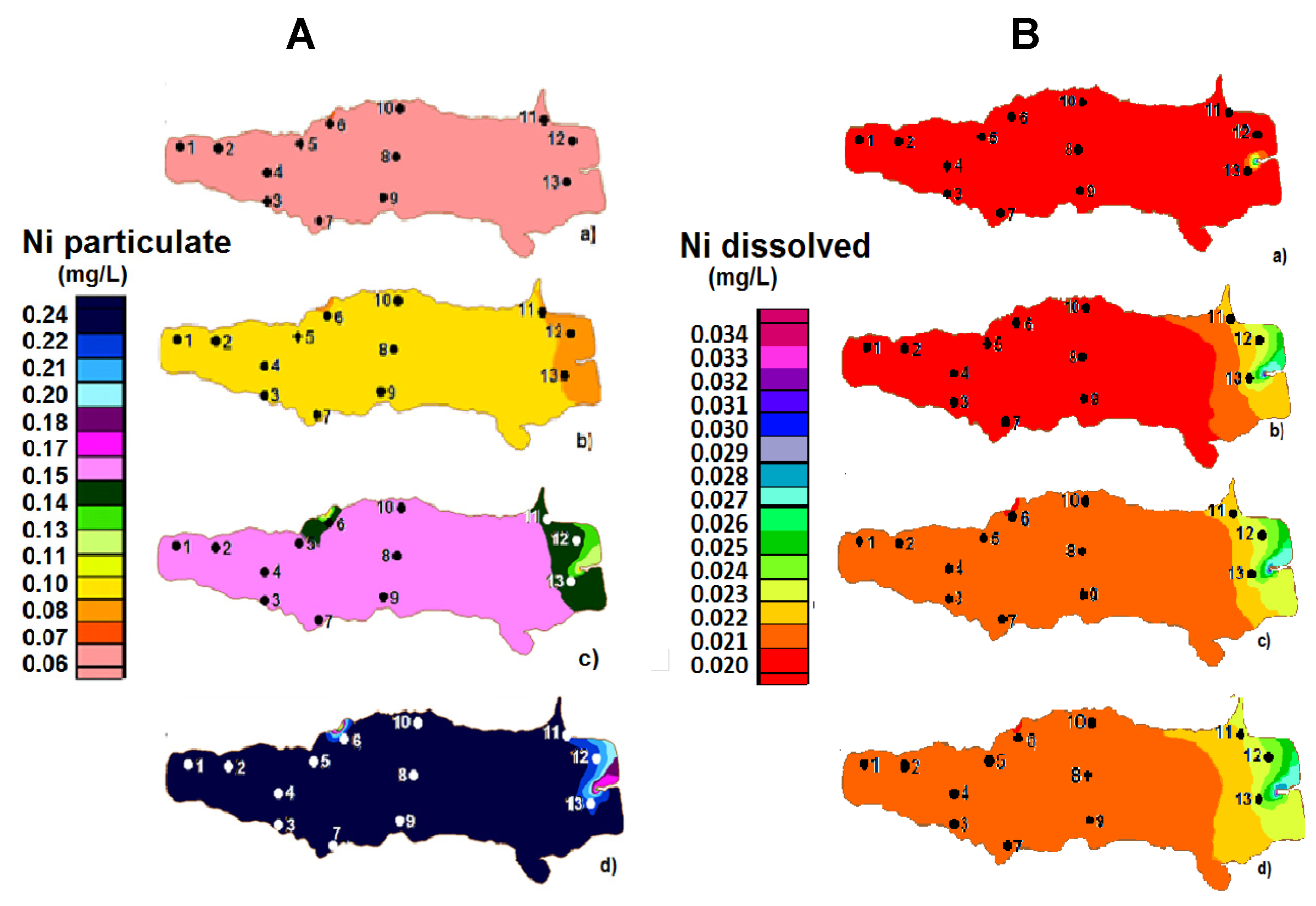
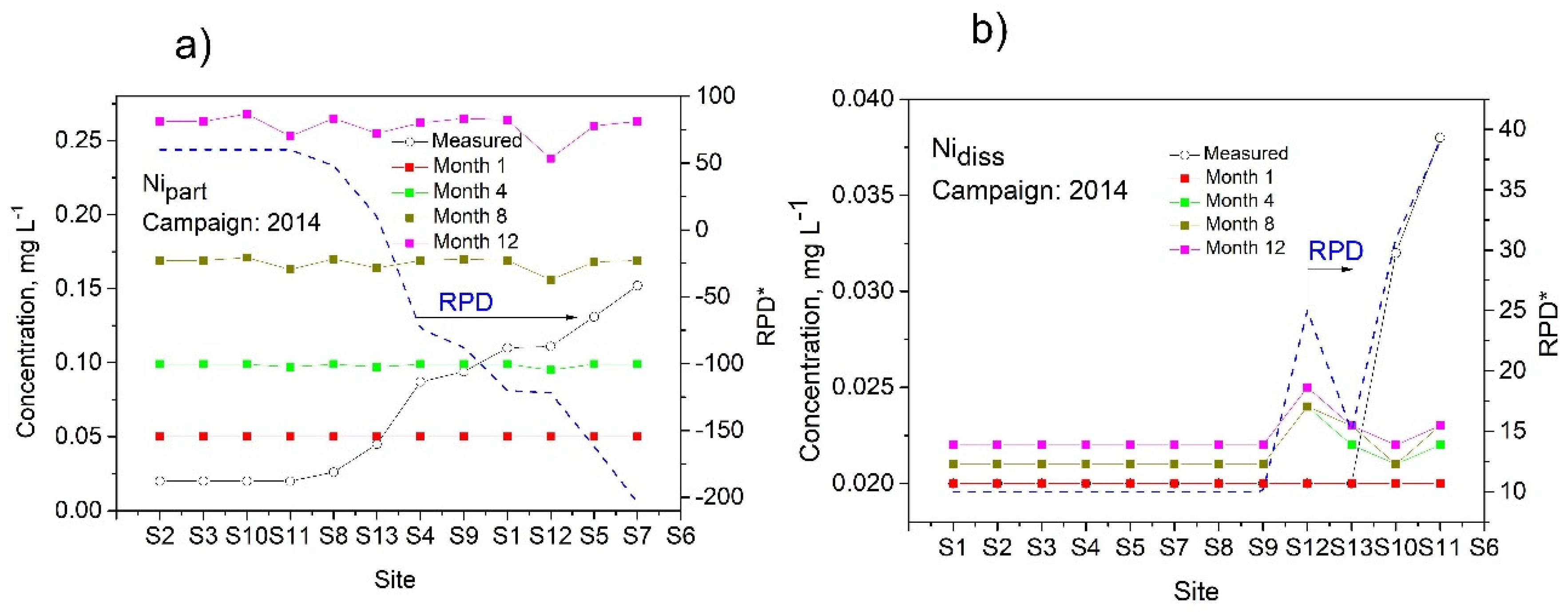
3.3.3. Nickel
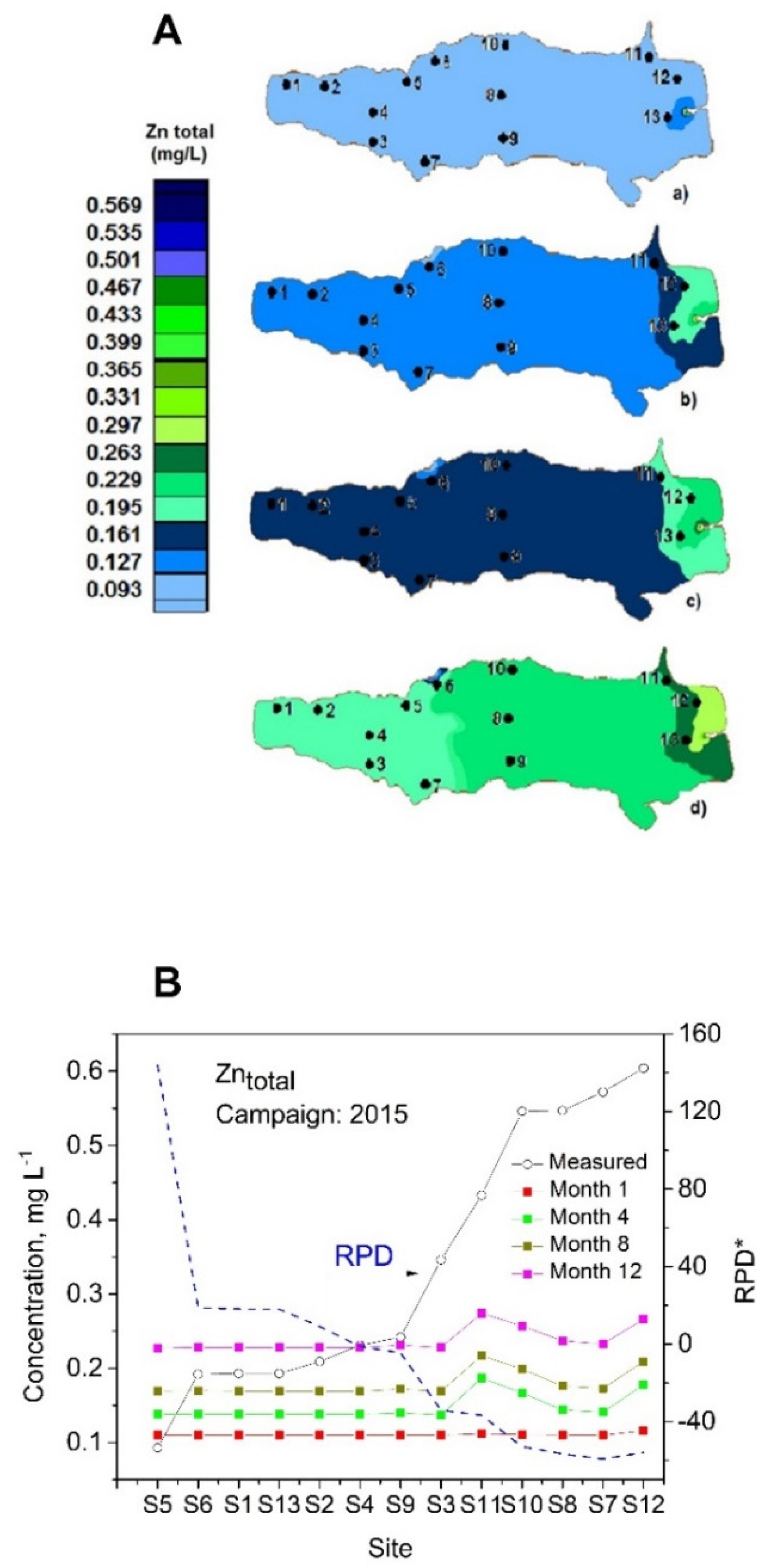
3.3.4. Zinc
4. Discussion
5. Conclusions
Supplementary Materials
Author Contributions
Funding
Data Availability Statement
Acknowledgments
Conflicts of Interest
References
- UN-Water. Global Annual Assessment of Sanitation and Drinking Water. 2010. Available online: http://whqlibdoc.who.int/publications/2010/9789241599351_eng.pdf (accessed on 3 March 2022).
- CNA. Agua en el Mundo, Cap 8. Water in the World. Chapter 8. 2011. Available online: http://www.conagua.gob.mx/conagua07/contenido/documentos/sina/capitulo_8.pdf (accessed on 12 March 2022).
- Hansen, A.M.; van Afferden, M. Modeling cadmium concentration in water of Lake Chapala, Mexico. Aquat. Sci. 2004, 66, 266–273. [Google Scholar] [CrossRef]
- Van Afferden, M.; Hansen, A.M. Forecast of lake volume and salt concentration in Lake Chapala, Mexico. Aquat. Sci. 2004, 66, 257–265. [Google Scholar] [CrossRef]
- Ma, L.; Lin, B.-L.; Chen, C.; Horiguchi, F.; Eriguchi, T.; Li, Y.; Wang, X. A 3D-hydrodynamic model for predicting the environmental fate of chemical pollutants in Xiamen Bay, southeast China. Environ. Pollut. 2019, 256, 113000. [Google Scholar] [CrossRef]
- Cowan-Ellsberry, C.; McLachlan, M.S.; Arnot, J.A.; MacLeod, M.; McKone, T.; Wania, F. Modeling exposure to persistent chemicals in hazard and risk assessment. Integr. Environ. Assess. Manag. 2009, 5, 662–679. [Google Scholar] [CrossRef]
- Liu, H.; Gopalakrishnan, S.; Browning, D.; Sivandran, G. Valuing water Quality change using a coupled economic-hydrological model. Ecol. Econ. 2019, 161, 32–40. [Google Scholar] [CrossRef]
- Hansen, A.M.; Maya, P. Adsorption-desorption behaviors of Pb and Cd in Lake Chapala, Mexico. Environ. Int. 1997, 23, 553–564. [Google Scholar] [CrossRef]
- Schneider, L.; Maher, W.A.; Floyd, J.; Potts, J.; Batley, G.E.; Gruber, B. Transport and fate of metal contamination in estuaries: Using a model network to predict the contributions of physical and chemical factors. Chemosphere 2016, 153, 227–236. [Google Scholar] [CrossRef]
- Ajiwibowo, H. Numerical model of sedimentation and water quality in Kerinci Lake. Int. J. GEOMATE 2018, 15, 77–84. [Google Scholar] [CrossRef]
- Jennings, A.A. Modelling sedimentation and scour in small urban lakes. Environ. Model. Softw. 2003, 18, 281–291. [Google Scholar] [CrossRef]
- Hillman, G.; Rodriguez, A.; Pagot, M.; Tyrrell, D.; Corral, M.; Oroná, C.; Möller, O. Simulación hidrodinámica bidimensional en la Laguna de los Patos, Brasil. MEC Comput. 2004, 23, 1233–1244. (In Spanish) [Google Scholar]
- Kuoe, J.; Shimadera, H.; Matsuo, T.; Kondo, A. Evaluation of thermal stratification and flow field reproduced by a three-dimensional hydrodynamic model in Lake Biwa, Japan. Water 2018, 10, 47. [Google Scholar] [CrossRef]
- Hansen, A.M.; van Afferden, M. Toxic substances. In The Lerma-Chapala Watershed: Evaluation and Management; Hansen, A.M., van Afferden, M., Eds.; Kluwer Academic/Plenum-Publishers: New York, NY, USA, 2001; Chapter 4. [Google Scholar]
- Jaishankar, M.; TTseten NAnbalagan BB Mathew, K.N. Beeregowda. Toxicity, mechanism and health effects of some heavy metals. Interdiscip. Toxicol. 2014, 7, 60–72. [Google Scholar] [CrossRef]
- Scott, C.A.; Silva-Ochoa, P.; Florencio-Cruz, V.; Wester, P. The Lerma-Chapala Watershed: Evaluation and Management; Hansen, A.M., van Afferden, M., Eds.; Kluwer Academic/Plenum Publishers: New York, NY, USA, 2001; Chapter 13. [Google Scholar]
- INEGI. Área Metropolitana de Guadalajara. 2020. Available online: https://www.jalisco.gob.mx/es/jalisco/guadalajara (accessed on 15 March 2022).
- SIAPA. Informe de Actividades y Resultados. Enero-diciembre de 2014. (Inform of Activities and Results. January–December 2014). 2014. Available online: https://www.siapa.gob.mx/sites/default/files/doctrans/informe_anual_2014_0.pdf (accessed on 10 March 2022). (In Spanish).
- Aparicio, J. Hydrology of the Lerma-Chapala watershed. In The Lerma-Chapala Watershed: Evaluation and Management; Hansen, A.M., van Afferden, M., Eds.; Kluwer Academic/Plenum Publishers: London, UK, 2001; pp. 3–30. [Google Scholar]
- Trujillo-Cardenas, J.L.; Saucedo-Torres, N.P.; Zárate del Valle, P.F.; Ríos-Donato, N.; Mendizábal, E.; Gómez-Salazar, S. Speciation and Sources of Toxic Metals in Sediments of Lake Chapala, Mexico. J. Mex. Chem. Soc. 2010, 54, 79–87. [Google Scholar] [CrossRef]
- DOF (Diario Oficial de la Federación). NMX-AA-014-1980: Cuerpos Receptores-Muestreo; DOF: Mexico, 1980. (In Spanish) [Google Scholar]
- Rice, E.W.; Baird, R.B.; Eaton, A.D.; Clesceri, L.S. (Eds.) Standard Methods for the Examination of Water and Wastewater, 22nd ed.; APHA, AWWA, WEF: Baltimore, MD, USA, 2012. [Google Scholar]
- USEPA. METHOD 3051 Microwave Assisted Acid Digestion of Siliceous and Organically Based Matrices. 2006. Available online: https://www.epa.gov/sites/production/files/2015-12/documents/3051a.pdf (accessed on 25 February 2022).
- US Army Corps of Engineers—Waterways Experiment Station Hydraulics Laboratory. RMA2, RMA4 WES Version 4.3; WesTech Systems Inc.: New York, NY, USA, 1997. [Google Scholar]
- Norton, W.R.; King, I.P. Operating Inst Ctions for the Computer Program RMA-2V; Resource Management Associates: Lafayette, CA, USA, 1997. [Google Scholar]
- Geankoplis, C.J. Transport Processes and Separation Process Principles, 4th ed.; Pearson: Boston, IN, USA, 2018. [Google Scholar]
- López Galván Edgar. Dissertation: Determinación de la Movilidad geo Hidrodinámica de Cd, Cu, Cr, Fe, Mn y Pb en la presa José Antonio Alzate en el Estado de México, México; Universidad Autónoma Metropolitana, Unidad Azcapotzalco: Mexico City, Mexico, 2010. (In Spanish) [Google Scholar]
- Corwin, D.L.; Vaughan, P.J.; Loague, K. Modeling Nonpoint Source Pollutants in the Vadose Zone with GIS. Environ. Sci. Technol. 1997, 31, 2157–2175. [Google Scholar] [CrossRef]
- Dickenson, J.A.; Sansalone, J.J. Discrete Phase Model Representation of Particulate Matter (PM) for Simulating PM Separation by Hydrodynamic Unit Operations. Environ. Sci. Technol. 2009, 43, 8220–8226. [Google Scholar] [CrossRef]
- CNA (Water National Commission). Bathymetric Map. Secretaria de Medio Ambiente y Recursos Naturale; CNA: Mexico City, Mexico, 2000. (In Spanish)
- Hosseiny, H. Implementation of heuristic search algorithms in the calibration of a river hydraulic model. Environ. Model. Softw. 2022, 157, 105537. [Google Scholar] [CrossRef]
- Abdullah, J.; Julien, P.Y. Distributed flood simulations on a small tropical watershed with the TREX model. J. Flood Eng. (JFE) 2014, 5, 17–37. [Google Scholar]
- Abdullah, J.; Muhammad, N.S.; Julien, P.Y.; Ariffin, J.; Shafie, A. Flood flow simulations and return period calculation for Kota Tinggi watershed, Malaysia. J. Flood Risk Manag. 2018, 11, S766–S782. [Google Scholar] [CrossRef]
- Filonov, A.E. On the dynamical response of Lake Chapala, Mexico to lake breeze forcing. Hydrobiologia 2002, 467, 141–157. [Google Scholar] [CrossRef]
- WMO (World Metrological Organization). Guide to Hydrological Practice, 6th ed.; No. 168; World Metrological Organization: Geneva, Switzerland, 2008; Volume I. [Google Scholar]
- López, D.L.; Gierlowski-Kordesch, E.; Hollenkamp, C. Geochemical Mobility and Bioavailability of Heavy Metals in a Lake Affected by Acid Mine Drainage: Lake Hope, Vinton County, Ohio. Water Air Soil Pollut. 2010, 213, 27–45. [Google Scholar] [CrossRef]
- Fortin, C.; Couillard, Y.; Vigneault, B.; Campbell, P.G.C. Determination of Free Cd, Cu and Zn Concentrations in Lake Waters by In Situ Diffusion Followed by Column Equilibration Ion-exchange. Aquat. Geochem. 2010, 16, 151–172. [Google Scholar] [CrossRef]
- De Anda, J.; Shear, H.; Maniak, S.; Riedel, G. Phosphorous balance in Lake Chapala (Mexico). J. Great Lakes Res. 2000, 26, 129–140. [Google Scholar] [CrossRef]
- Roldan-Perez, G.; Ramirez Restrepo, J.J. Fundamentos de Limnología Neotropical, 2nd ed.; Editorial Universidad de Antioquia: Medellín, Colombia, 2008; pp. 244–246. (In Spanish) [Google Scholar]
- Pauer, J.J.; Auer, M.T. Nitrification in the water column and sediment of a hypereutrophic lake an adjoining river system. Water Res. 2000, 34, 1247–1254. [Google Scholar] [CrossRef]
- Chapra, S.C. Surface Water-Quality Modeling; McGraw-Hill International Editions: Singapore, 1997. [Google Scholar]
- De Anda, J.; Maniak, U. Alterations of the hydrologic regime and their effects in the phosphorus and phosphates in lake chapala, Mexico. Interciencia 2007, 32, 2. Available online: http://ve.scielo.org/scielo.php?script=sci_arttext&pid=S0378-18442007000200007 (accessed on 12 March 2022).
- Ryding, S.O.; Rast, W. The Control of Eutrophication of Lakes and Reservoirs; Man and the Biosphere Series; UNESCO/Parthenon: París, France, 1989; Volume 1, 314p.


Disclaimer/Publisher’s Note: The statements, opinions and data contained in all publications are solely those of the individual author(s) and contributor(s) and not of MDPI and/or the editor(s). MDPI and/or the editor(s) disclaim responsibility for any injury to people or property resulting from any ideas, methods, instructions or products referred to in the content. |
© 2023 by the authors. Licensee MDPI, Basel, Switzerland. This article is an open access article distributed under the terms and conditions of the Creative Commons Attribution (CC BY) license (https://creativecommons.org/licenses/by/4.0/).
Share and Cite
Alvarez-Bobadilla, J.I.; Murillo-Delgado, J.O.; Badillo-Camacho, J.; Barcelo-Quintal, I.D.; Valle, P.F.Z.-d.; Reynaga-Delgado, E.; Gomez-Salazar, S. Modeling Fate and Transport of Nutrients and Heavy Metals in the Waters of a Tropical Mexican Lake to Predict Pollution Scenarios. Water 2023, 15, 1639. https://doi.org/10.3390/w15091639
Alvarez-Bobadilla JI, Murillo-Delgado JO, Badillo-Camacho J, Barcelo-Quintal ID, Valle PFZ-d, Reynaga-Delgado E, Gomez-Salazar S. Modeling Fate and Transport of Nutrients and Heavy Metals in the Waters of a Tropical Mexican Lake to Predict Pollution Scenarios. Water. 2023; 15(9):1639. https://doi.org/10.3390/w15091639
Chicago/Turabian StyleAlvarez-Bobadilla, Jorge I., Jorge O. Murillo-Delgado, Jessica Badillo-Camacho, Icela D. Barcelo-Quintal, Pedro F. Zárate-del Valle, Eire Reynaga-Delgado, and Sergio Gomez-Salazar. 2023. "Modeling Fate and Transport of Nutrients and Heavy Metals in the Waters of a Tropical Mexican Lake to Predict Pollution Scenarios" Water 15, no. 9: 1639. https://doi.org/10.3390/w15091639