New Software for the Techno–Economic Analysis of Small Hydro Power Plants

Guzović, Zvonimir; Barbarić, Marina; Bačelić Medić, Zlatko; Degiuli, Nastia

doi:10.3390/w15091651

Open AccessArticle

New Software for the Techno–Economic Analysis of Small Hydro Power Plants

by

Zvonimir Guzović

^*,

Marina Barbarić

,

Zlatko Bačelić Medić

and

Nastia Degiuli

Faculty of Mechanical Engineering and Naval Architecture, University of Zagreb, Ivana Lučića 5, 10000 Zagreb, Croatia

^*

Author to whom correspondence should be addressed.

Water 2023, 15(9), 1651; https://doi.org/10.3390/w15091651

Submission received: 3 March 2023 / Revised: 7 April 2023 / Accepted: 12 April 2023 / Published: 23 April 2023

(This article belongs to the Special Issue Sustainable Development of Water, Energy, and Environment Systems)

Download

Browse Figures

Versions Notes

Abstract

:

Project SMART (Strategies to Promote Small-Scale Hydro Electricity Production in Europe) from the Intelligent Energy Europe (IEE) program, in which 7 institutions from 5 European states participate, pointed to the important barriers for the expansion of small hydro power plants (SHP) in Europe. One of the main barriers is the lack of suitable methodology and software able to create a clear view of the SHP potential in the given territory, as well as a complete techno-economic analysis for certain locations. Worldwide, there are a certain number of software for this purpose, and will be presented in this paper. However, in practical application for concrete cases, they show certain disadvantages. For example, one software is not able to take into account all the specifics of watercourses and plants; another does not have the option of selecting all types of turbines; in others, the calculation models are based on a limited number of equations that do not describe all possible cases; in some, economic analysis is oversimplified, etc. The aim of this paper is to develop software that is more comprehensive than any existing software. A new software for the techno-economic analysis of SHP is developed using Python and will be presented in this paper. The software is very useful for experts in the field of SHP, but also much wider, for decision-makers, potential investors, and stakeholders, especially in developing countries. It will improve water resources management, disseminate opportunities to investors, and increase the interest of stakeholders to invest in SHP, resulting in their wider use. The software is tested on location for SHP in the Republic of Croatia by comparison with the results obtained by the usual classical calculation. The agreement of the results is satisfactory.

Keywords:

renewable energy; small hydro power plants (SHP); SMART project; techno–economic analysis; new software (tool)

1. Introduction

Today, the world is entering a new era [1,2]:

Climate change represents the most pressing existential threat to humanity;
An era of low-carbon energy, characterized by dramatic changes in the energy supply–demand relationship;
About 770 million people still do not have access to clean, affordable, and reliable electricity, and almost one in three people do not have access to safely managed drinking water;
The Paris Agreement also includes the transition from fossil to renewable energy sources;
As a renewable energy, hydropower plays an essential role in decarbonization of the energy system (especially small hydro power plants (SHP)) and play an important role for the global energy supply;
Driven by the increasing demand for energy and global climate change, many countries have given priority to hydropower development in the expansion of their energy sectors.

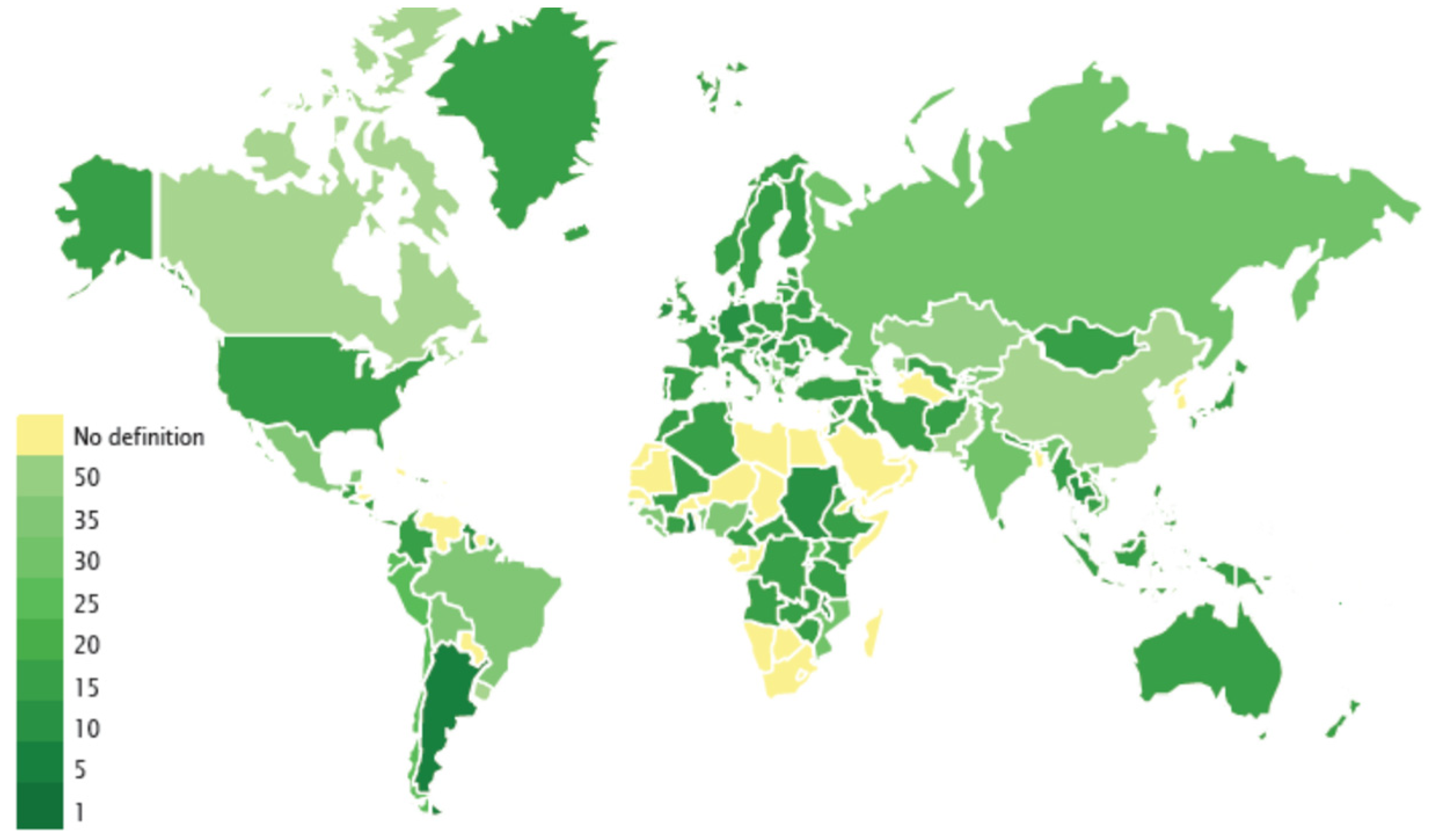
There is still no universal international definition for SHP, but it is generally defined by generating capacity with upper limits varying from 10 to 50 MW. In particular, SHP by definition in many countries refers to plants with power below 10 MW, as presented in Figure 1 [1].

Characteristics of SHP are [3,4]:

A mature technology which can easily be designed, operated, and maintained locally;
Economically feasible and has minimal impact on the environment;
Contributes greatly to solving the problem of rural electrification, improving living standards and production conditions, promoting rural economic development, alleviating poverty, as well as reducing emissions;
Favoured by the international community, especially by developing countries;
Has the lowest electricity generation prices of all offgrid technologies, and the flexibility to be adapted to various geographical and infrastructural circumstances.

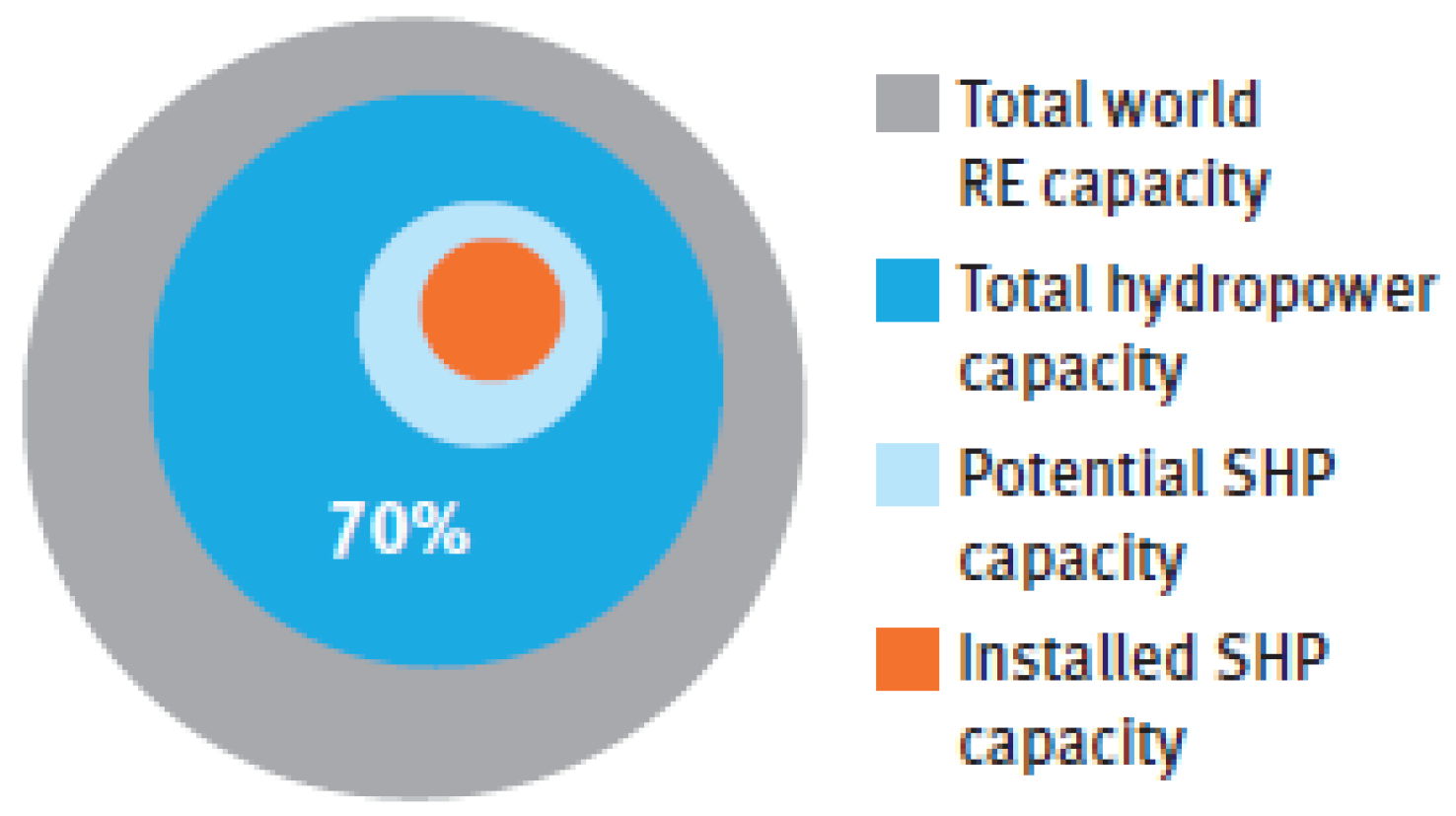
The global installed SHP capacity for plants up to 10 MW is estimated at 78 GW [1]. SHP represents only approximately 1.5% of the world’s total electricity installed capacity, 4.5% of the total renewable energy capacity, and 7.5% (<10 MW) of the total hydropower capacity [1]. Despite the appeal and benefits of SHP solutions, much of the world’s SHP potential remains untapped (66%), especially in developing countries as shown in Figure 2 [1].

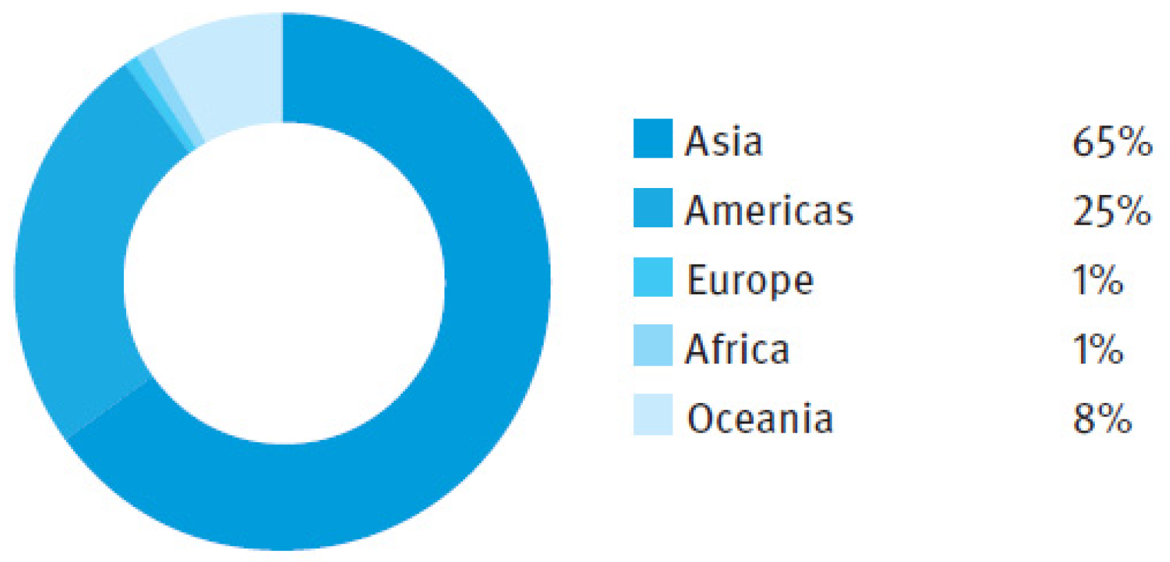
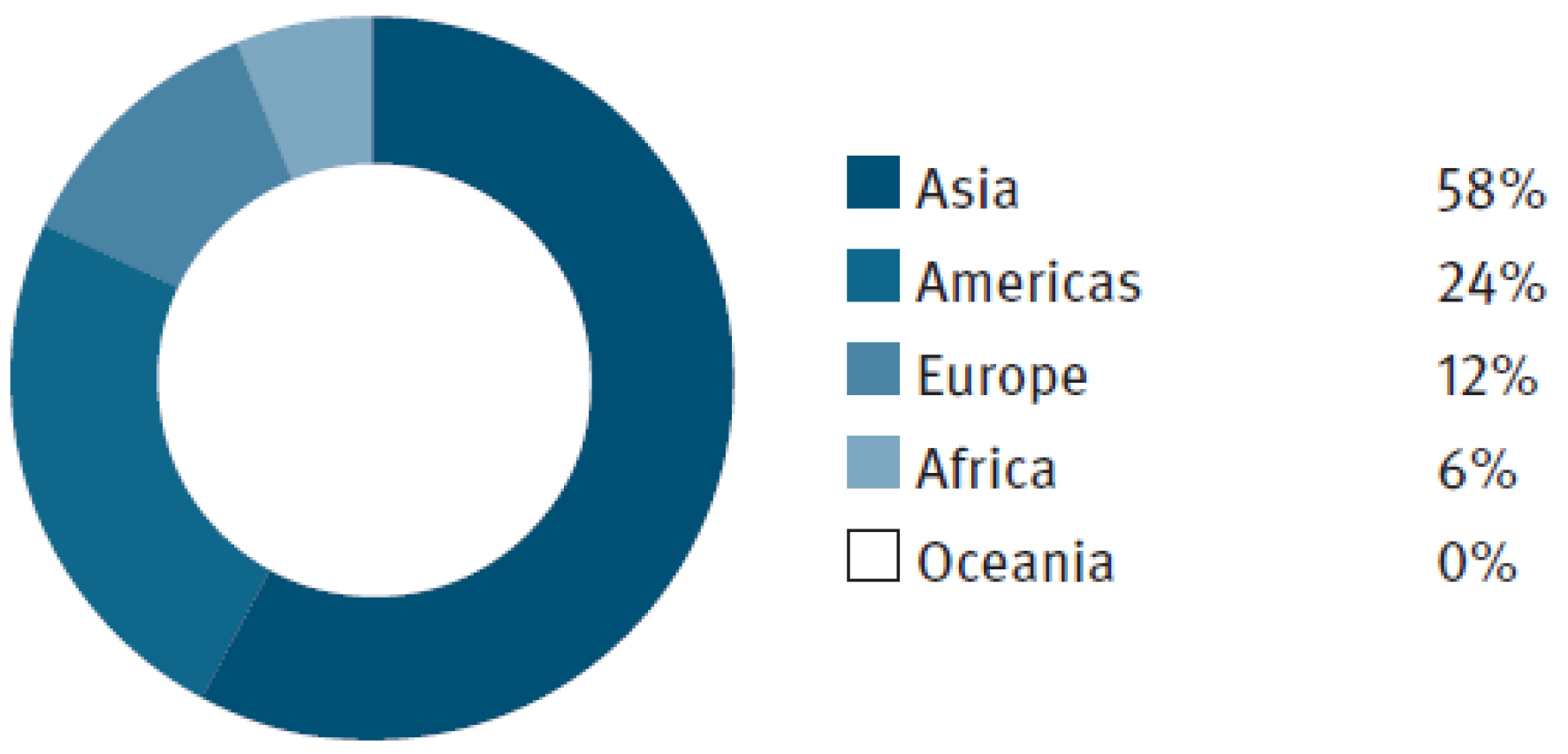
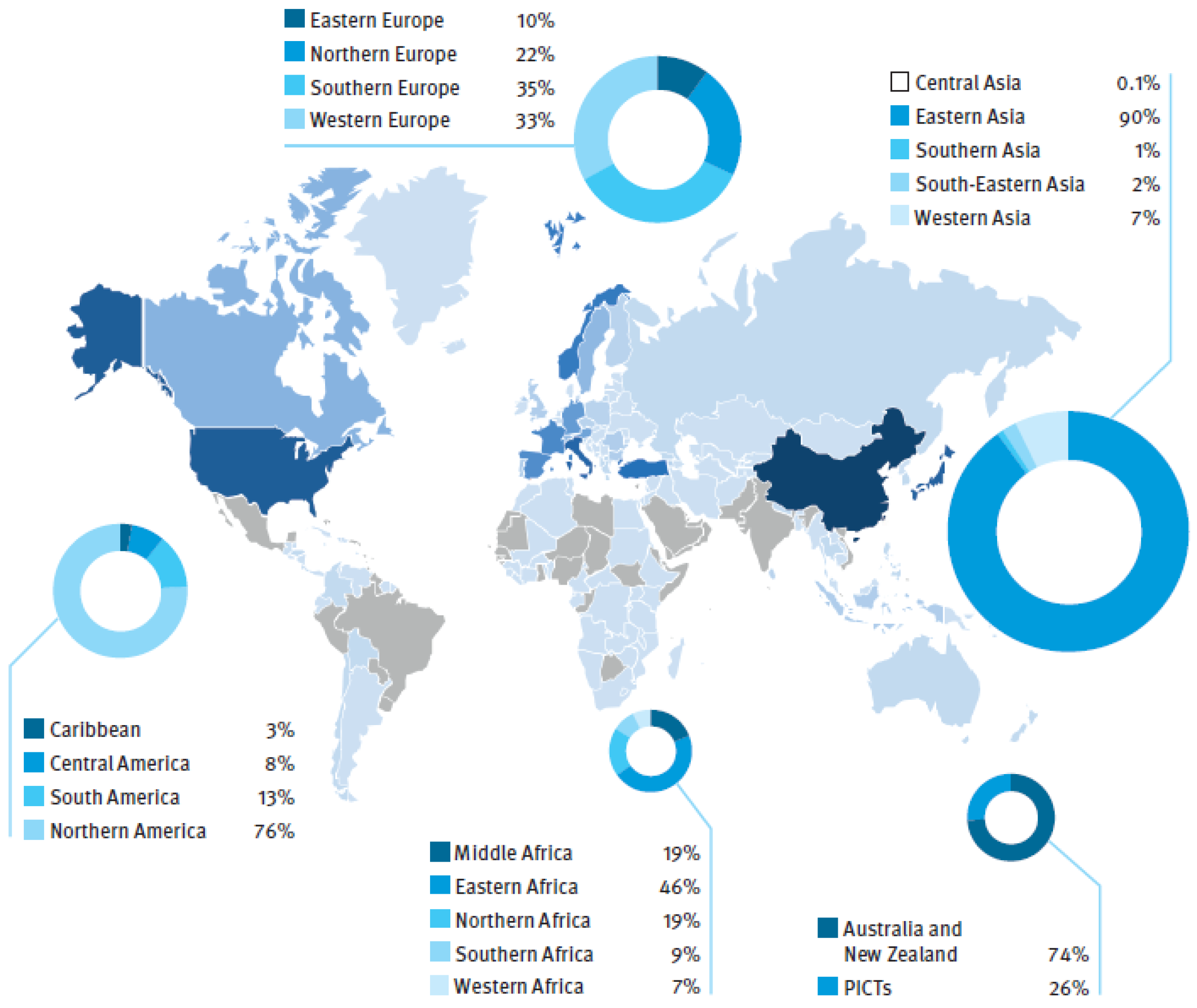
Asia continues to have the largest installed capacity and potential for SHP up to 10 MW, as shown in Figure 3 [1].

Europe has 88% of its potential already developed, as shown in Figure 4 [1].

The top six countries—China, the United States of America (USA), Japan, Italy, Norway, and Turkey—account for 67% of the world’s total installed capacity of SHP [1]. China with 54% of the world’s total installed capacity (definition of up to 10 MW) has more than four times the SHP installed capacity of Italy, Japan, Norway, and the USA combined [1]. Figure 5 presents installed SHP up to 10 MW capacities worldwide [1].

The Congress Draft of the San José Declaration on Sustainable Hydropower (World Hydropower Congress 7–24 September 2021) stated that “Sustainable hydropower is a clean, green, modern and affordable solution to climate change. Going forward, the only acceptable hydropower is sustainable hydropower [5]”. The question is: can SHP be sustainable [6,7]?

The assessment of hydropower sustainability was modeled in [8]. To assess run-of-river SHP potential in South Sudan, the Soil and Water Assessment Tool (SWAT) model was used in [9]. Recently, the potential for the exploitation of excess (and wasted) energy sources in existing hydropower facilities has been increasingly considered in Europe [10].

The assessment of SHP sites for development represents a relatively high proportion of overall project costs [11,12,13]. A high level of experience and expertise is required to accurately conduct this assessment. The methodology and analysis of risk factors for the initial cost assessment of hydropower is proposed in [14], to enable project developers to identify critical areas for detailed investigations. A quantification of the ecological impact of SHP based on the integrated approach is presented in [15]. A case study on the implementation of a hydropower plant in Switzerland, concentrated mostly on the effectiveness of policies for increasing use of renewable energy, is presented in [16]. The reasons behind the slow progress of the hydropower sector in Pakistan were investigated and presented in [17], while a case study of status and potential of SHP in Southern African development community was presented in [18]. Results regarding local views on run-of-river hydropower in German, Portuguese, and Swedish case studies, which are relevant for hydropower operators and policymakers, are presented in [19]. However, in the conclusion of the paper, it is pointed out that further investigation is required for specific national case studies not discussed in the work.

Over the last several decades, a variety of computer-based assessment tools (software) have been developed, which enable a prospective developer to make an initial assessment of the economic feasibility of a project before spending substantial sums of money. These software range from simple first estimates to quite sophisticated programs. However, a reliable assessment of real economically feasible potential implies some “on the ground” surveying of possible sites and their electricity generation potential. Thus, the appearance of Geographic Information System (GIS) software has been of enormous use as a way of capturing the range of information required. These technologies can store spatial catchment information of a proposed SHP site in a GIS database and use it for decisions on whether to proceed with SHP plant development. GIS tools coupled with a hydrological tool is proposed in [20] to detect potential locations for a run-of-river plant.

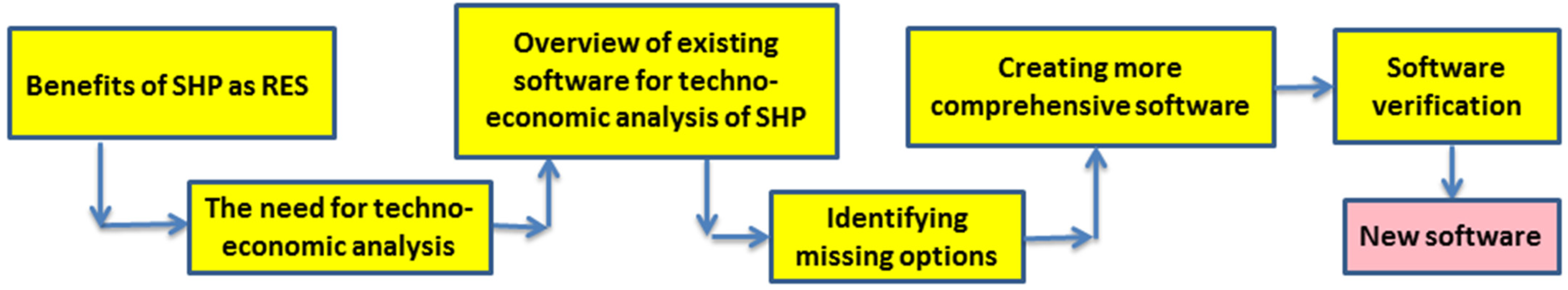
Although there are a certain number of software packages, which will be presented in this paper, project SMART has detected the lack of suitable, complete methodology and software (tools) for techno-economic analysis of SHP for certain locations. Every one of them shows certain disadvantages, and they are not able to take into account all the specifics of watercourses. For example, one software is not able to take into account all the specifics of watercourses and plants (e.g., derivation channel of open type with different cross-sections); another does not have the option of selecting all types of turbines (e.g., novel very low head turbines) and different numbers of installed turbines; in others, calculation models are based on a limited number of equations that do not describe all possible cases (e.g., calculation of minimum biological flow, pressure losses in individual components, etc.); in some, economic analysis is oversimplified, etc. The aim of this paper is to develop software that is more comprehensive than any existing software, which is indicated by the equations given in the appendix, on which individual modules are based. In this way, it replaces the simultaneous use of multiple software. New software for the techno-economic analysis of SHP is developed using Python and will be presented in this paper. The interface of the software is also designed to allow appropriate application. The software is very useful for experts in the field of SHP, but also much wider for decision-makers, potential investors, and stakeholders, especially in developing countries where “Engineers without Borders” are involved in this type of project. It will improve water resources management, disseminate opportunities to investors, and increase the interest of stakeholders to invest in SHP, resulting in their wider use. The software is tested on location for SHP in the Republic of Croatia by comparison with the results obtained by the usual classical calculation. The agreement of the results is satisfactory. The diagram in Figure 6 illustrates the whole idea of new software development presented in this paper.

2. Existing Software for the Analysis of SHP

Software for the techno-economic analysis of SHP are often developed for specific conditions in countries around the world, and currently no single tool has been found that has been shown to meet all the requirements for preliminary analysis of SHP. Accordingly, two or more software are often used to harmonize the obtained data, technical and economic, in order to obtain complete and satisfactory results [21]. In order to reveal the advantages and disadvantages of the tools available on the market, an analysis and description of each tool is presented below.

2.1. Conventional Software Tools for SHP Assessment

Computer software designated for SHP assessment can be integrated or not into GIS (i.e., using the spatial data of a catchment). To assess river flow, there are two main approaches: the flow duration curve (FDC) and the simulated streamflow (model) methods. A less accurate intermediate approach is based on the mean annual flow (MAF), which can also be used in some programs. Table 1 summarizes the software packages applied for hydropower studies [11].

2.1.1. SMART Mini-Hydro

SMART Mini-Hydro [22] is a software for techno-economic analysis of SHP developed as part of the SMART project, co-financed by the Intelligent Energy Europe program. SMART Mini-Hydro is a tool in MS Office Excel format, and therefore has certain limitations; however, it contains a large amount of calculation modules.

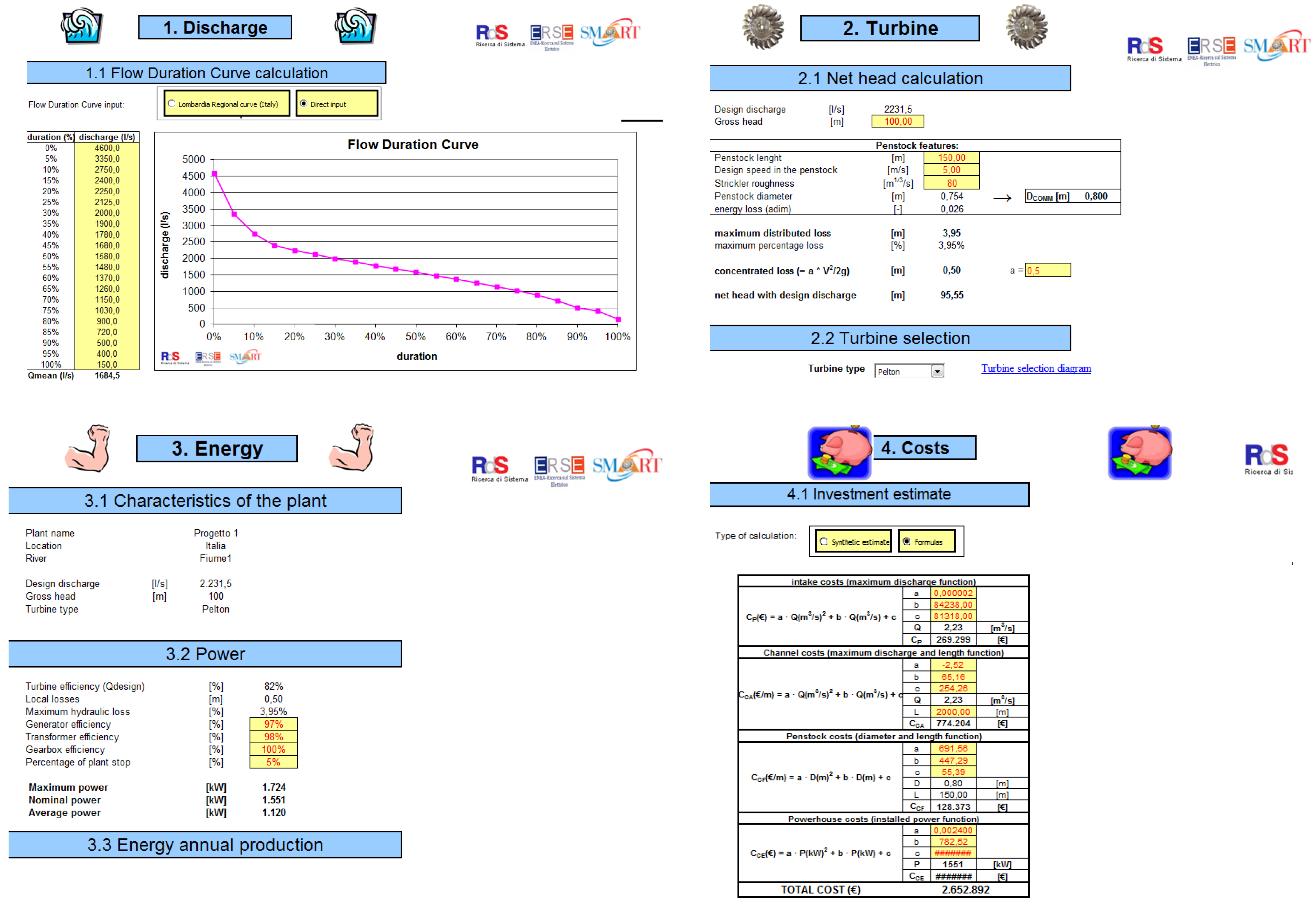
The tool consists of modules divided according to the calculation of relevant parameters—flow, geodesic head, turbine, produced electricity, costs and economic analysis, as shown in Figure 7 [22]. In more detail, work in the tool begins by defining the flow duration curve according to the defined intervals, after which the tool displays the curve graphically. Below are the calculations of the flow of the biological minimum, the net flow, and the entry or calculation of the designed flow of a SHP. This is followed by the calculation of flow losses and the calculation of the geodetic head. Finally, the calculation of technical parameters and the amount of electricity produced ends after selecting the desired type of turbine. The cost calculation and financial analysis are quite concise, and only the basic costs of the intake (function of flow), pipelines (function of diameter and length), and powerhouse (function of installed turbine power) are calculated.

The advantages of this tool are certainly the detailed calculation procedures of technical parameters and a very good presentation of the obtained results; however, in some parts, the presentation of individual calculation steps is missing for a better understanding of the tool and the SHP. Additionally, the absence of an integrated diagram for turbine selection, which is set in the tool as an external reference, is considered a drawback, and the user is not able to see the exact parameters of a SHP on the diagram. In addition to the above, the calculation procedure for determining flow losses in open channels that are used in Croatia is missing.

2.1.2. RETScreen International Clean Energy Project Analysis Software

RETScreen International Clean Energy Project Analysis Software is a tool developed for the purpose of promoting projects of renewable energy sources and energy efficiency and unifies budgeting procedures for making techno-economic analyses of various technologies and projects [23,24].

The tool also includes databases for renewable energy projects where users can see the specifics of each created case. Furthermore, the tool includes the characteristics of the necessary machines in order to obtain the most accurate calculation of technical and economic parameters. The tool is available in a large number of world languages.

The RETScreen Small Hydro Project model can be used at any location to evaluate grid-connected, isolated-grid, or off-grid SHP projects. The tool offers the possibility to select the size of the turbines, as well as the number of turbines required, whether it is a large-, medium-, or micro-SHP project. The problem with RETScreen appears when trying to discover the methodology used to calculate quantities in hydropower projects. In addition, since it is a tool for various projects of renewable energy sources, some details that would need to be shown in the preliminary analysis are excluded.

2.1.3. Small Hydropower Plant Software—NTNU

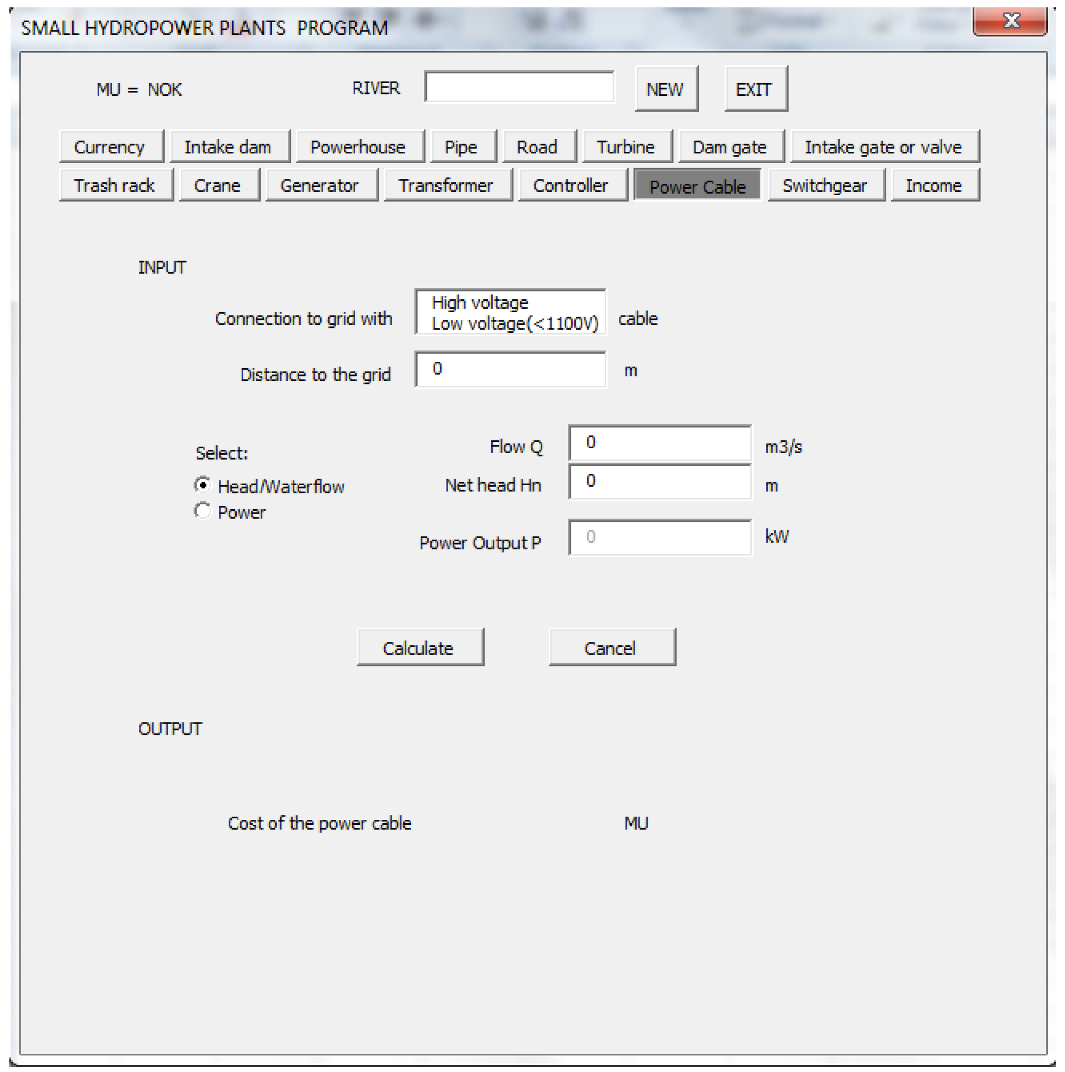
This software [22] was also developed as part of the SMART project and represents a significant step towards the calculation of the costs of the considered plant. The tool is based on the MS Office Excel program package, and a separate user interface has been developed for use, which significantly simplifies the use of the tool, as shown in Figure 8 [22].

The tool is able to create a detailed calculation of all parts of a SHP, with specific application to the territory of Norway. Although very easy to use, the tool does not offer the possibility of more detailed calculation of the technical parameters of the planned plant, which can be cited as the main drawback. Furthermore, the tool lacks calculation procedures that would enable the calculation of economic parameters of specific components, for example, new types of turbines that are coming into use. The tool offers the possibility of plant optimization taking into account both the technical and economic parameters of the planned plant.

2.1.4. HydroHELP Design Cost Tool

The HydroHELP Design Cost Tool [25] is a series of tools developed for use in calculating parameters that allow the engineer to make a preliminary estimate of a SHP with a minimum amount of location data. The tool is intended for relatively experienced engineers with guidelines for creating an analysis. All tools in the HydroHELP series were created using the MS Office Excel software package. The tools do not include analysis of hydrological or financial data.

Currently, the HydroHELP series consists of four tools:

HydroHELP 1.4 for turbine selection;
HydroHELP 2.4 for Francis turbines;
HydroHELP 3.4 for impulse turbines;
HydroHELP 4.4 for Kaplan turbines.

The calculation procedure begins with a turbine selection tool that suggests the most suitable turbine to the user for the defined parameters of flow, net drop, and number of turbines in a SHP. After this step, according to the tool recommendation, the user is directed to calculation tools for a specific type of turbine—for calculation of Francis turbines, for calculation of impulse turbines, and for calculation of Kaplan turbines.

The above tools guide the user through the calculation and design process while offering the best options for all components. Input hydrological data are taken from maps and site visits without geotechnical investigations. The tools have been successfully tested on several projects.

2.1.5. Integrated Method for Power Analysis (IMP 5.0)

IMP [26,27] is a computer tool for site assessment for SHP projects. By using the IMP tool in combination with meteorological and topographic data, it is possible to create a quick assessment of a potential location. The tool includes electricity generation estimation, flood frequency curve creation, and fish habitat analysis.

IMP is usable for users without experience in SHP to discover potential locations for projects, for learning, and for experts in the field of SHP. The IMP tool, as mentioned earlier, consists of:

models for flood frequency analysis;
models for the analysis of the flow duration curve (FDC) and hourly and daily flow values based on data on precipitation, temperatures, and the description on the left;
a simulation model for estimating electricity production from the collected data on a daily or annual level;
fish habitat analysis module.

2.1.6. PEACH Software

This tool is dedicated to preliminary studies of hydropower sites [28,29]. It considers all technical engineering methods, usually used at these preliminary stages, and also deals with economic and financial analysis of hydropower schemes.

2.1.7. The Hydropower Evaluation Software (HES)

This tool enables the user to account for environmental, legal, and institutional constraints in the USA [30]. It uses environmental attributes and federal land code data to generate a project environmental suitability factor.

2.2. GIS Applications for Evaluating Hydropower Potential

The latest computer-based packages have integrated GIS tools or vice versa—some of them are a part of GIS. Table 2 presents GIS-based Small Hydropower Atlases on the Internet [11].

2.2.1. NVE Atlas

To fully understand the potential for small hydro (50 kW to 10 MW), the Norwegian Water and Energy Directorate (NVE) developed a new method for resource mapping using GIS technology between 2002 and 2004 [31,32,33,34]. The method involved identifying waterfalls with the potential for hydro development and then adding available hydrological data and cost figures for intakes, waterways, and power stations. ArcGIS standard hydrologic analysis was used to derive runoff. Certain limitations were set with regard to the river slope, elevation, run-off volume, maximum usable flow, installed power, and production. The plant design was fixed automatically as soon as the head and flow were known, and the power output and generation capacity was automatically calculated.

2.2.2. The Rapid Hydropower Assessment Model (RHAM)

Developed by KWL [35], it is used to assess the run-of-river hydroelectric potential for the province of British Columbia (BC), Canada, for an area of approximately 950 thousand square kilometres [36]. Over 8000 potential hydroelectric opportunities were identified. A powerful geographic information systems-based computer model enabled the assessment to be completed in four months. RHAM is developed using an ArcGIS 9.2 platform with the Spatial Analyst extension from ESRI Canada. GIS data sources incorporated into the model included DEM data from Natural Resources Canada and hydrology data from the B. C. Ministry of Environment.

2.2.3. The Virtual Hydropower Prospector (VHP)

It is a GIS application designed to assist users in locating and assessing natural stream water energy resources in the United States [37,38]. It was developed as part of the Small Hydropower Resource Assessment and Technology Development Project conducted at the Idaho National Laboratory (INL) with the support of the USA Department of Energy Wind and Hydropower Technologies Program. The intended use of VHP is to obtain a broad overview of water energy resources in an area of interest or to perform a preliminary development feasibility assessment of particular sites of interest. The location of features and the associated attribute information are for indication only. Actual on-site locations, measurements, and evaluations must be undertaken to verify information presented by VHP and assess true development feasibility.

2.2.4. Hydrobot

It is a combined GIS and financial assessment tool to identify micro-hydro schemes [39]. It was first conceived as a university project and operated as a series of processes rather than a single model. The model was first used for a study commissioned by the Forum for Renewable Energy Development in Scotland on behalf of the Scottish Government to assess the nation’s remaining hydro potential [40]. Hydrobot can be applied to any land area within Scotland and the top sites supplied to those developers. Hydrobot is based on a surface flow model derived from elevation data in a 10 m × 10 m grid across the whole of Scotland. Every watercourse has been modelled to give the FDC at any point. The accuracy of the predicted flows has been tested against measured flows away from established gauging stations and also examined by the Scottish Environmental Protection Agency.

2.2.5. VAPIDRO ASTE

A methodology to evaluate the residual hydropower potential in Italy, taking into account the current uses (such as irrigation and drinking water), with a numerical technique coupled with a GIS was proposed. It is an interactive GIS and web-based map, called VAPIDRO ASTE [22,41]. VAPIDRO ASTE is a numerical tool that allows for the evaluation of the residual potential hydropower energy and all possible alternatives concerning the sites for hydroelectric plants along the drainage network. The model applied through GIS technology coupled the hydrological and hydrographical characteristics of nearly 1500 interconnected sub-basins and rainfall maps. Maps of maximum and residual hydropower potential were produced and were found to be quite helpful tools to support the power authorities’ decision makers and other stakeholders in creating energy master plans and in implementing SHP.

3. New Software (Tool) for Techno-Economic Analysis of SHP

The techno-economic analysis of SHP includes the consideration of hydrological parameters with the aim of exploiting a certain water flow for the purpose of electricity production and defining the estimated technical and assumed economic parameters. Through analysis, it is possible, with certain assumptions, to obtain preliminary energy results and economic results by establishing functional dependence on energy results.

With such analyses, it is possible to obtain information about the hydrological parameters of a certain water flow (flow, design flow, biological minimum flow, etc.), losses in the planned plant (flow losses in pipelines or channels), turbine type, turbine target parameters, plant power, and the total available annual amount of electricity that can be produced. It is necessary to emphasize that with this analysis it is not possible to obtain detailed results for each individual part of a SHP, but rather approximate results that can differ to a certain extent from those obtained by calculation and proper dimensioning of individual components of a SHP. The primary goal of such analyses is to obtain preliminary results that will provide the user with a more detailed insight into the possibilities of exploiting the targeted water flow, i.e., its energy potential. As will be shown in the following chapters, the software (tool) is flexible when it comes to certain calculation modifications according to user requirements, and the graphical interface is made simple and user-friendly. The software is designed to guide the user through the process of creating a techno-economic analysis of the planned SHP, indicating the parameters that the user must enter. Moreover, the transparency of calculating procedures enables the user to have a deeper understanding of the topic and to quickly obtain results for the planned plant.

In the modules for economic analysis, the parameters relevant to the project assessment and decision-making on the implementation of the project are calculated. Of course, the assessment of the investment in such cases, without the obtained data, will depend on the pre-entered equations that are listed in the methodological overview of the software in the appendix. Inaccuracies introduced by approximations and the application of equations can give a completely wrong picture of investment costs; therefore, the software allows for corrections of each of the cost groups in order to enable a more accurate calculation of costs. When considering this segment of software, it is necessary to take into account that obtaining accurate data is a demanding task, and that it depends solely on previously acquired experiences and preferred suppliers of equipment and/or works and services.

Detailed analyses of each component of a SHP require a large amount of knowledge, experience, and time, as well as quality data that the user is able to properly change with the aim of optimizing the plant, whether it is optimization of the technical part of the process or optimization of investment costs.

3.1. Software Structure

Structurally, the software is designed in such a way that it guides the user through the calculation of all relevant parameters, and that by entering certain required data, it simultaneously displays solutions, which greatly contributes to the possibility of optimizing the planned plant. The need for user interaction and data entry is minimized by applying equations that significantly simplify the calculation process. Of course, with such a method, certain deviations will appear in the calculation; however, it is recognized that the level of accuracy of the results provided by the software meets the ultimate purpose—the analysis of the potential of a certain water flow.

The first version of the software was developed primarily for use in Croatia. It was developed in Microsoft Office Excel which has significant limitations, but still offers quite satisfactory possibilities for structuring such a software. The second version of the software (v.2.0.), that will be presented in this paper, has been developed in Python. The method and equations are given and explained in the appendix. The standard Python GUI Interface, Tkinter, was used, as well as some standard libraries to perform mathematical operations: NumPy and NumPy financial. The second version of the software has been expanded with some additional features and adapted for international use. The transparency of the calculation process itself gives the user better insight into all the parameters of the planned plant and requires a certain level of prior knowledge in order to use it properly.

The software algorithm consisting of seven modules is shown in Figure 9. The modules are Net/designed flow module, Net head module, Turbine module, Energy production module, Investment module, Financial and economic module, and Sensitivity analyse module.

3.2. Net/Designed Flow Module

The net flow module is structured in such a way that it guides the user through the calculation procedure and the determination of the design flow Q_DES, which is the relevant quantity for further calculation. By calculating and visualizing all the necessary values, the entire procedure is facilitated. In Appendix A, Appendix B and Appendix C, there is an explanation of the calculation process in this module.

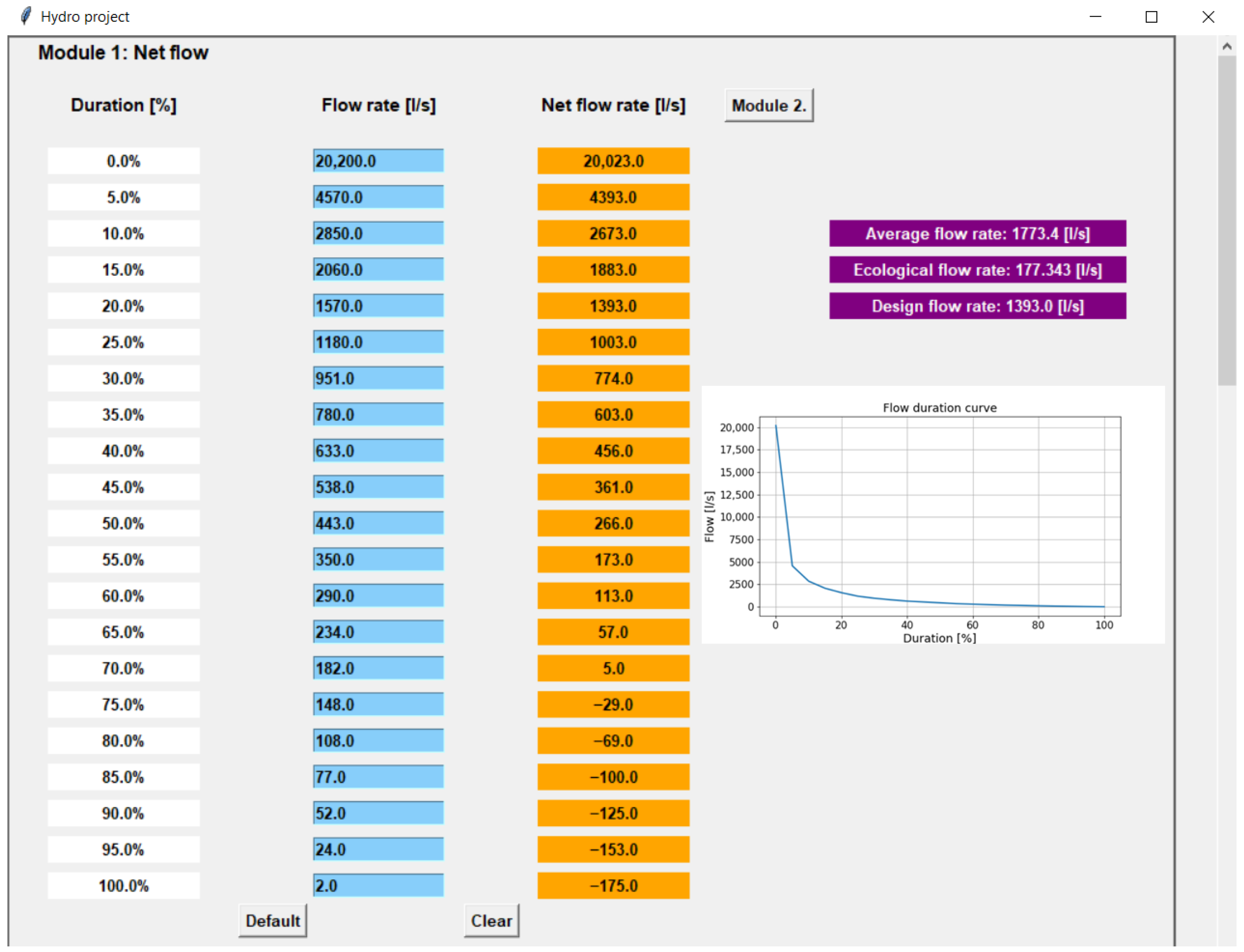
The calculation procedure begins with the entry of data for the flow duration curve (FDC), where the data of the flow duration curve from 0–100% is entered in the cells provided for this with a step of 5% [42]. After entering all values, the FDC is graphically displayed and the average flow rate Q_AV is calculated. The user interface of the calculation procedure for the FDC and average flow is presented in Figure 10.

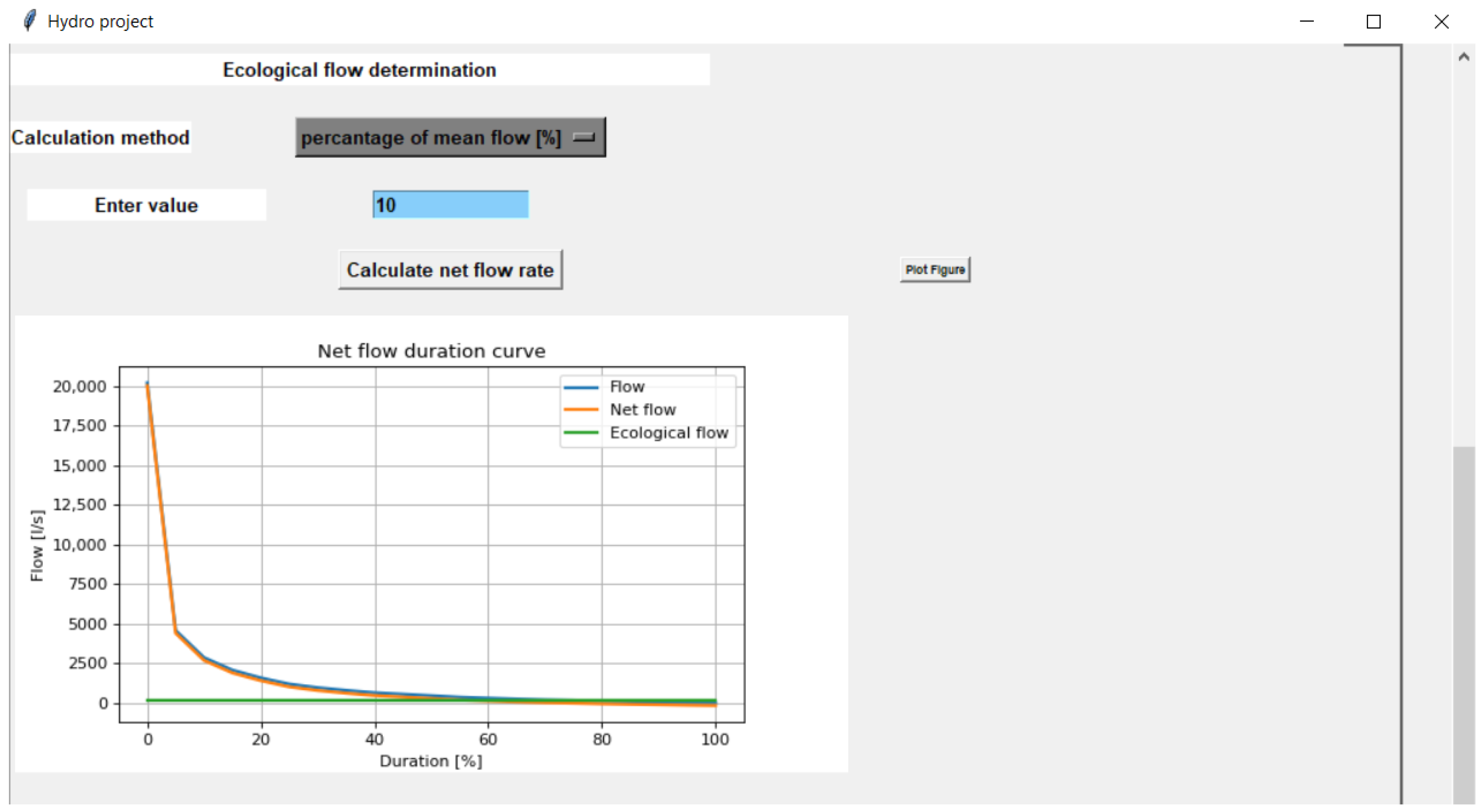
The ecological flow Q_ECO is an item that must be included in the calculation procedure since it is necessary to meet the ecological requirements [43]. Some of the methods that can be used in the calculation are given in Appendix B. The user interface for calculation of the ecological flow is presented in Figure 11.

In the software, it is possible to choose the method of calculating the flow of the ecological minimum, and it is up to the user to decide which method to use. The ecological minimum flow can be calculated in two ways:

According to the desired share in the calculated average flow.
Direct user input of the desired value.

The selection of the two mentioned methods of calculating the flow of the ecological minimum takes place using the drop-down menu.

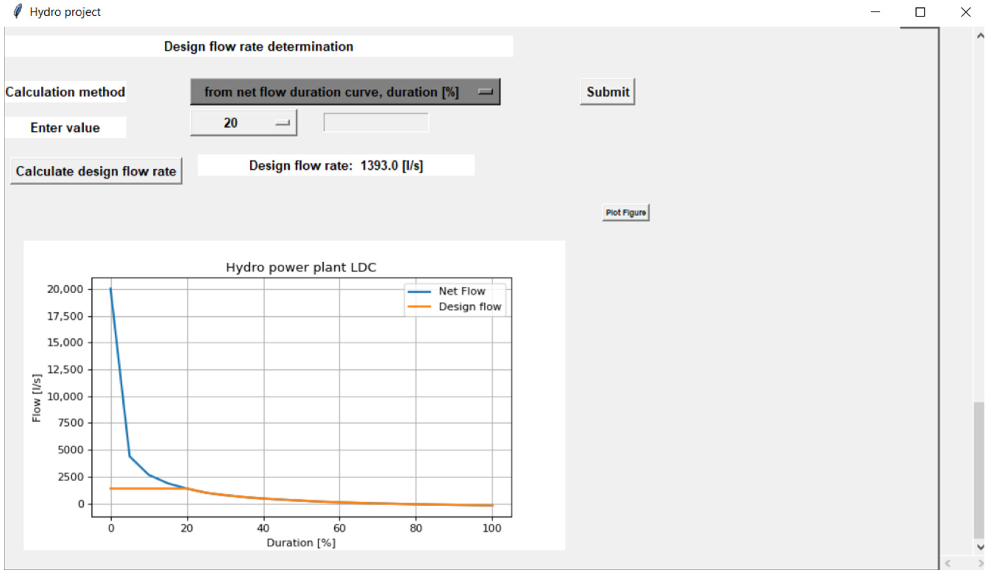
Further calculation includes the calculation of the net flow (the flow entered in the flow duration curve minus the flow of the ecological minimum at each moment of the flow duration) and defining the value of the designed flow.

The user has the option of choosing two methods of calculating the design (project) flow Q_DES, as shown in Figure 12:

Direct manual input of the designed flow value.
Calculation of the value of the designed flow according to the duration in the flow duration curve.

Regardless of the method chosen for determining the design flow, the software graphically displays curves to the user, based on which the correctness of the data can be observed.

3.3. Net Head Module

In the net head module, the task is to determine the flow losses in the supply structures [44,45,46,47], in accordance with methodology presented in Appendix D. The input data for the calculation includes the natural geodetic head h_GEO that the user enters, and the previously calculated design flow Q_DES.

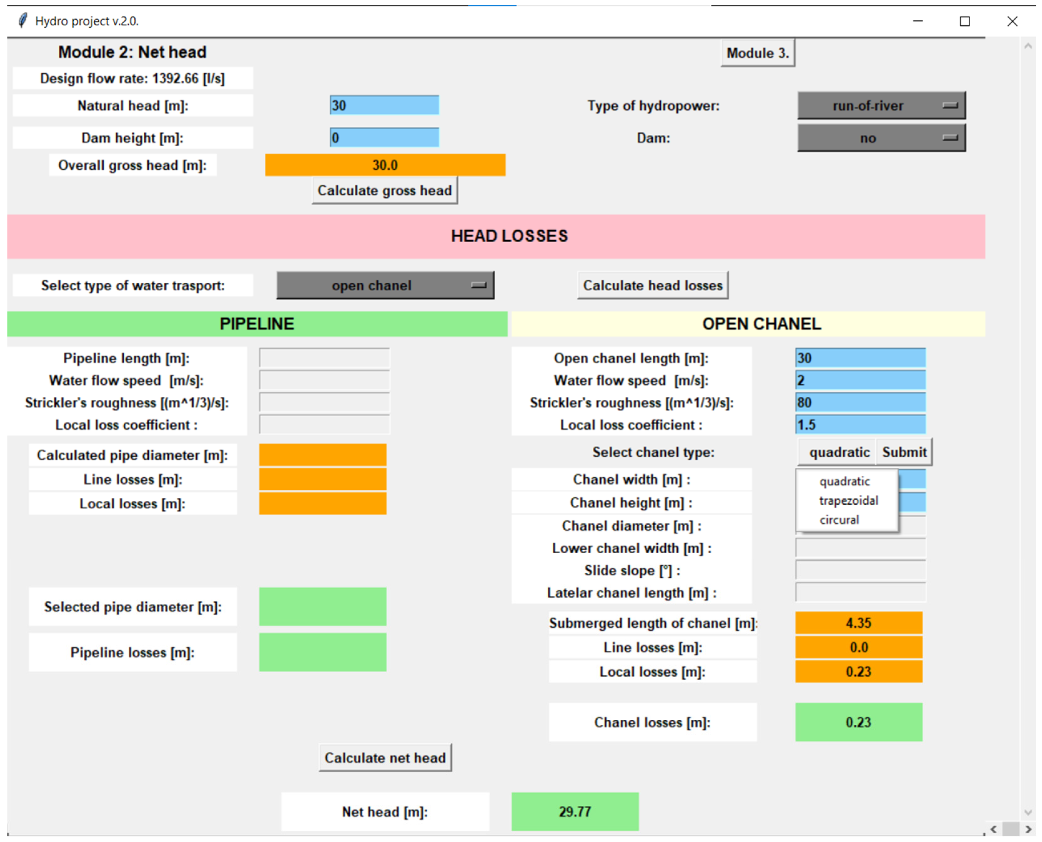
The first step in this calculation module is the selection of the type of power plant, i.e., run-of-the-river or diversion SHP. If it is run-of-the-river SHP, depending on the location conditions, it is not necessary to calculate the head losses. If it is a diversion SHP, it is necessary to calculate the flow losses since the lengths of the supply structures can often be very large. It is possible to increase the natural geodesic head with a dam, which is also made possible by the software. The next step in the calculation is the entry of the measured geodetic head at the location. To this value, if the user has chosen the existence of a dam, the value of the hydraulic height of the dam is added to obtain the total value of the geodetic head. By selecting and entering these parameters, it is possible to continue with the calculation of flow losses, where it is necessary to choose the actual type of structure— channel or tunnel—with an open water surface or under pressure. The selection is made before the loss calculation itself, and the user is enabled to calculate the selected option. When calculating the losses of pressure in channels/tunnels, the user is required to enter the length of the channel/tunnel, the design velocity, roughness, and the coefficient of local losses. Based on these data, the diameter of the pipeline, as well as line and local flow losses, are calculated. The sum of these two losses gives the total losses, and they are subtracted from the given total geodetic head. It is the same with the calculation for supply structures with an open water face, with the difference that it is necessary to specify the dimensions of the channel/tunnel since the losses depend on the shape of the cross-section and other relevant parameters. It is left to the user to choose which cross-section will be used; it is possible to choose between square, circular, and trapezoidal cross-sections. It should be noted here that for the same imposed conditions of designed flow and geodesic head, the losses in supply structures with an open water face will be lower compared with the losses calculated in pressurized supply structures.

The user interface of the calculation procedure for flow losses, i.e., net head h_NET is presented in Figure 13.

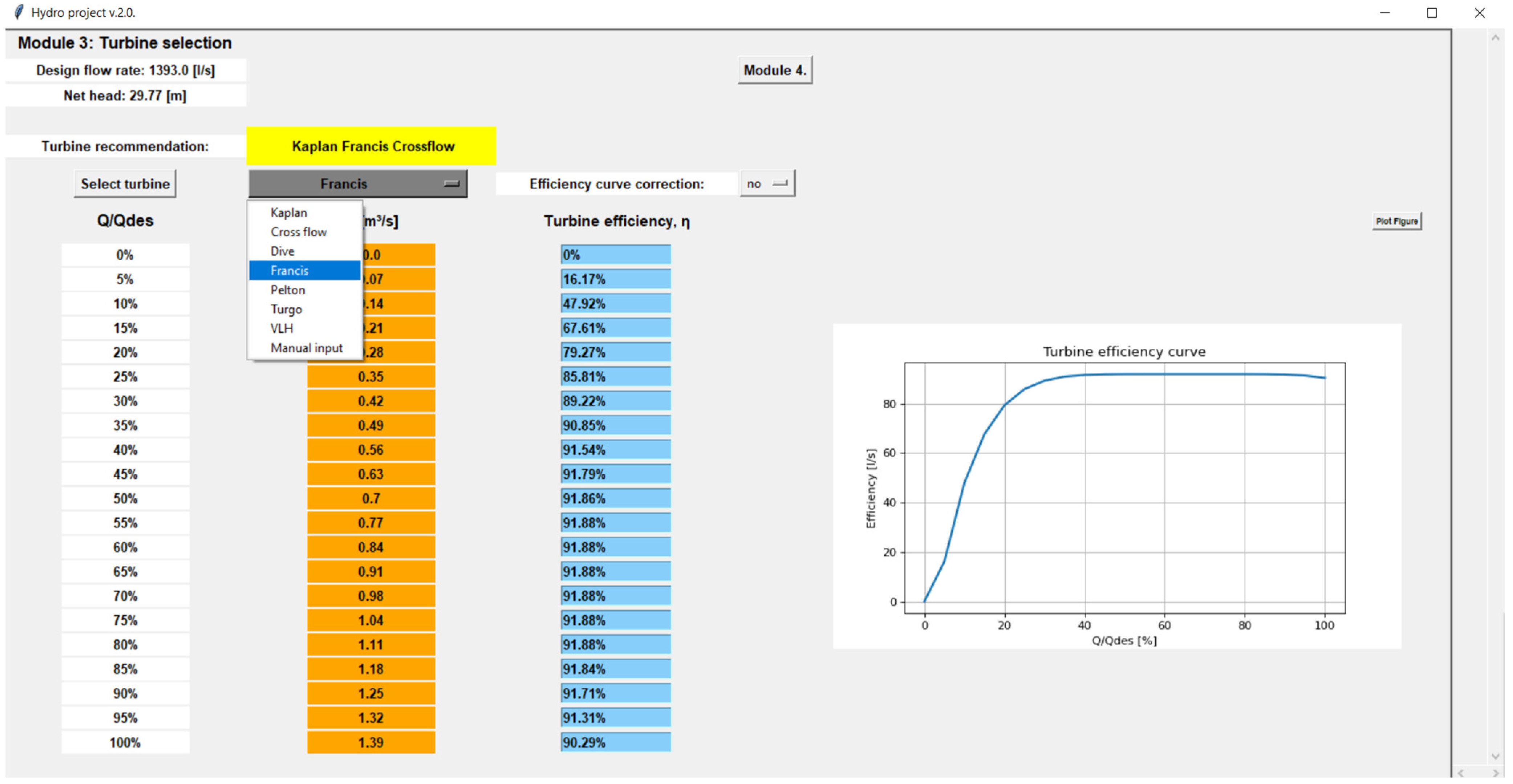
3.4. Turbine Module

In this software module, the user determines the desired type of turbine in accordance with the parameters of the geodetic head and the design flow, with an overview of all relevant parameters of each type of turbine that can be selected in the software. By choosing the appropriate turbine, the user directly affects the resulting power of the plant, and the investment costs related to the plant itself. In order to simplify the turbine selection process for the user, two possible ways of consideration are available. The first includes the proposal of turbines whose working area corresponds to the parameters of the geodetic head and the design flow, and the second is the selection of the appropriate type of turbine according to the turbine selection diagram.

After deciding on the appropriate turbine for application in a specific case, the user is required to define the type of turbine via a drop-down menu. By selecting one of the offered types of turbines, the user can view data on the efficiency of the turbine, i.e., the efficiency curve of the turbine. Such a curve shows the efficiency of the selected turbine at a certain percentage point of the designed flow, which defines all relevant parameters. The data used for the efficiency curve of the turbines used in the software may differ from the actual data due to the existence of a large number of different machines belonging to the same turbine group. Due to this, the user is enabled to correct the previously entered data of the efficiency curve of the turbine if they have a higher quality data set or data obtained directly from the manufacturer. The correction is applied through the drop-down menu and by opening the possibility of entering the efficiency value for a certain percentage of the design flow.

The user is also able to choose the number of turbines that are planned up to a maximum value of 10 turbines. For each of the turbines, it is necessary to enter what proportion of the design flow they take, and what is the minimum flow through each individual turbine. By entering the specified parameters, a diagram is displayed on which for each selected turbine the surface of the share of flow that they take over at a particular moment of the flow’s duration is drawn. The user interface of the turbine module for users (decision-makers, potential investors, and stakeholders) is presented in Figure 14.

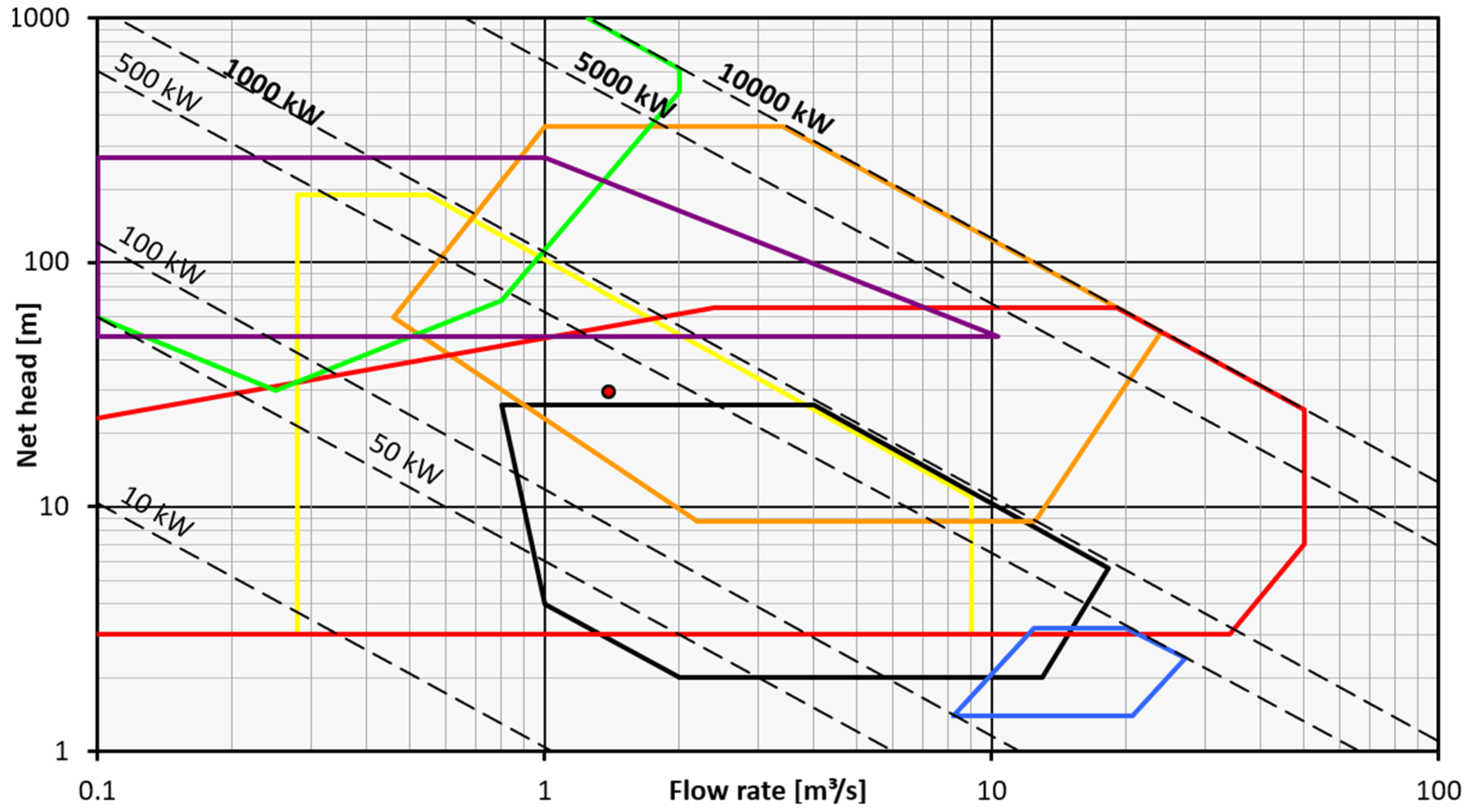
3.5. Turbine Selection Module

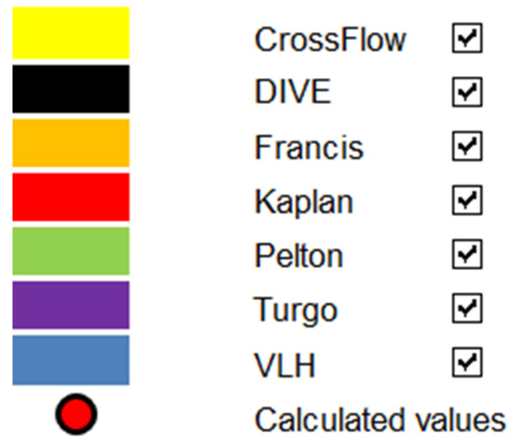
The turbine selection module is directly related to the previous turbine module and serves as an auxiliary module to guide the user in selecting the appropriate turbine according to the turbine selection diagram, i.e., the declared working areas of individual types of turbines. The data used to create the turbine selection diagram was taken from data on individual types of turbines, as well as measured or calculated values of previously available turbine selection diagrams. Deviations in the entered values of the diagram for the selection of turbines are possible; however, it is estimated that the values are accurate enough to correctly decide on the appropriate type of turbine in a particular case. Nonetheless, it is necessary to take into account that the actual data of the turbine manufacturer may differ and go outside the marked working areas of the particular type of turbine. Since collecting data on all individual turbines of each manufacturer of the same type of turbine is not possible, a solution is resorted to that fits and significantly simplifies the process of selecting the appropriate machine. It should also be noted that with some turbines, the operating area is determined according to the manufacturer’s data. Examples of this include the DIVE and VLH turbines, where data on the working area is publicly available on the Internet addresses of individual manufacturers. The turbine selection diagram is made in logarithmic scale on both axes, where the abscissa axis indicates the flow and the ordinate axis the geodesic head that can be used. As can be seen below, the basic possibilities of displaying sizes in the diagram have been extended by programming code to achieve a higher level of interaction with the user. The diagram contains all the turbines that can be used in the software, the lines indicating the power of the turbines, and the display of previously calculated or entered operating parameters of the plant (design flow and geodetic head). The mentioned parameters are entered or calculated in the previously described software modules and are taken as such to represent the possible operating point of the plant. A higher level of interaction is achieved by adding programming code that allows the user to “hide” the characteristics of all turbines shown on the diagram. Specifically, the initial presentation of the diagram with the characteristics of all turbines seems quite confusing due to the large number of lines, and it seems quite a difficult task to determine in which operating area the operating point of the plant falls, as shown in Figure 15. Precisely for this reason, it is possible to “hide” the characteristics of each individual turbine, which makes the selection of the appropriate turbine significantly simpler. The mentioned function of the module is made possible, as mentioned earlier, by adding the corresponding program code which, with the help of the associated checkbox elements, removes the characteristic or displays it in the diagram.

In the diagram above, the turbines are marked with different colors according to the legend in Figure 16.

The data used for the turbine selection diagram is also the starting point for the function by which the software automatically suggests to the user the turbines that can be used according to the operating point parameters of the SHP. For example, for the parameters shown in the diagram above, the software suggests the use of Francis- or Turgo-type turbines, which corresponds to the visual representation in the diagram. This procedure provides the user with a further simplification of the selection of an appropriate turbine and serves as the first step for orientation. The result of this function is printed in the turbine module. This module contains a quick link to return to the turbine module.

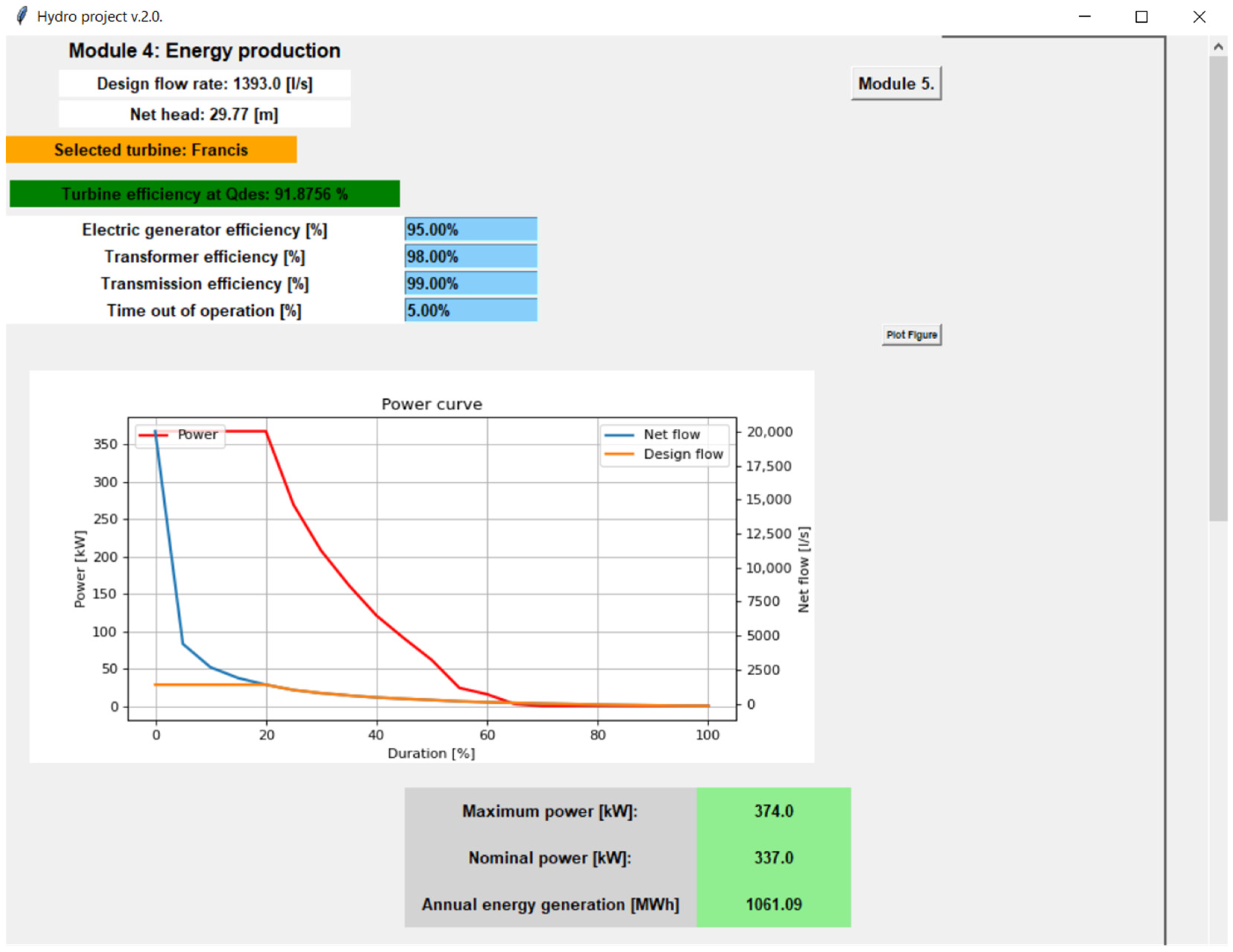
3.6. Energy Production Module

The energy production module calculates the final annual amount of electricity produced.

Before calculating the total amount of energy produced during the year, the user is shown all the parameters of the plant for each individual turbine, depending on the number of turbines selected. Net head and flow inputs are taken from previous calculations, as well as turbine data. The user is required to define the efficiency of the components that affect the energy production after the turbine:

Generator efficiency;
Transformer efficiency;
Transmission efficiency.

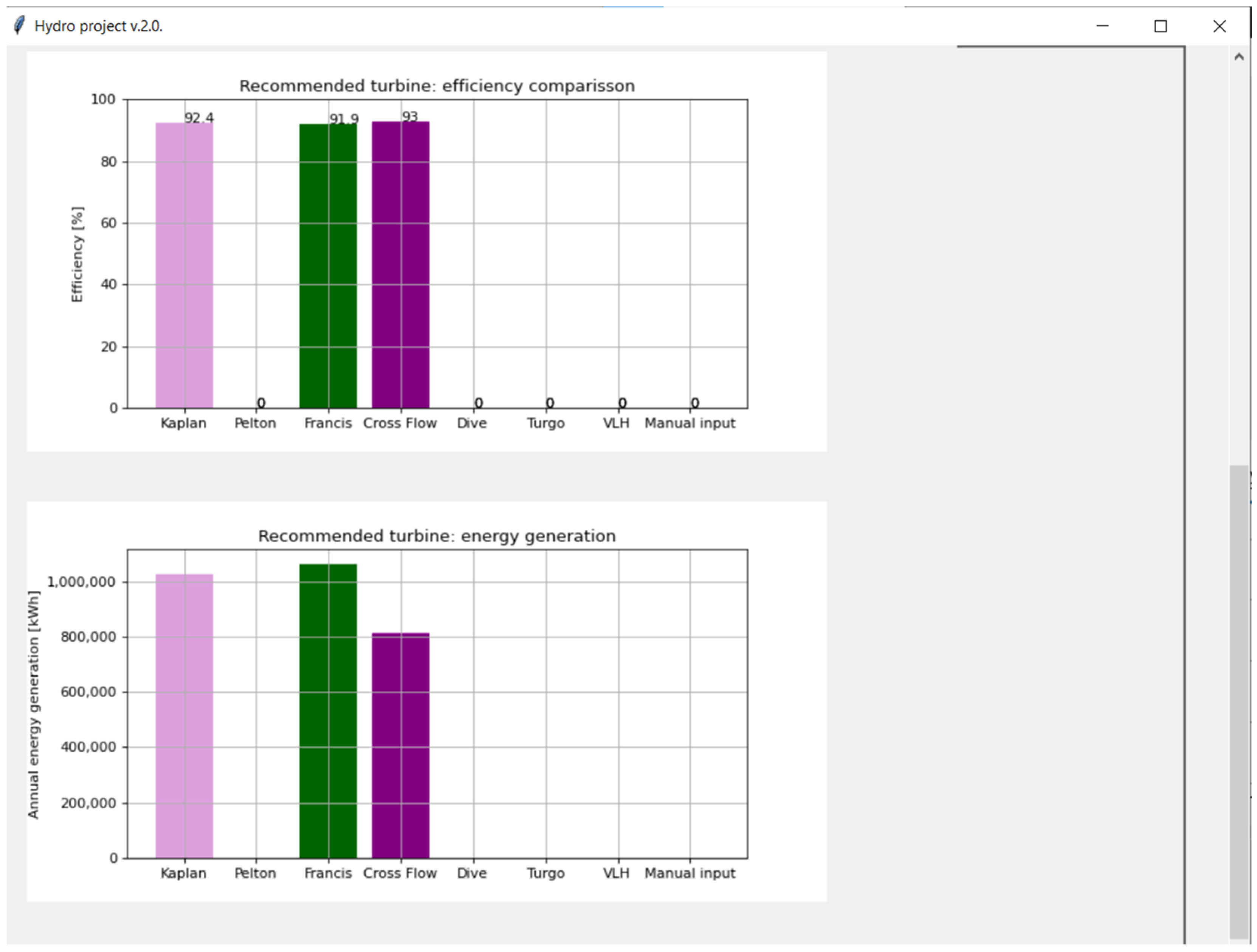
Additionally, it is necessary to define the time during which a SHP is out of operation, since the total amount of energy produced is calculated for 100% availability of the plant. In the further steps of this module, the user is not required to enter any further parameters. In the continuation of the module, it is possible to display all relevant parameters of the plant, as well as a comparison of the plant with the selected turbine and a plant with other turbines that can operate in the defined area (net flow and net head).

More about the energy production module can be found in Appendix E. The user interface of the energy production module is presented in Figure 17.

3.7. Investment Module

By estimating the investment costs based on the entered and calculated technical parameters, the basis for further economic analysis and evaluation of the project is realized. Investment costs are divided into groups and the following are considered [44,45,46,47]:

Dam construction costs;
Costs of construction of the catchment structure;
Construction costs of the power plant building;
Turbine, generator and transformer costs;
Costs of supply and drainage structures;
Costs of other mechanical and electrical equipment;
Cost of work, services, and design.

Due to the relatively large possibility of error in the calculation of the cost of each individual group, the user is left with the option of correcting the cost of each group according to the desired/obtained data. Of course, equally, even with corrected data, there is a possibility of making an error in the investment calculation. Entering other parameters is actually not necessary, since the calculation of investment costs itself is automated, but it depends on the wishes of the user. More about the investment module can be found in Appendix F.

3.8. Financial and Economic Module

The financial and economic module is included in the tool to display all relevant parameters of the financial and economic evaluation of the plant. This module requires a relatively large number of data to enter since there are a large number of parameters that depend on the user’s judgment. The module uses the data obtained from the previous investment module for the calculation of cash flows in selected time periods, while defining other necessary data.

Other required data for entry includes data on the credit, expected lifetime of the plant, plant costs, plant production, and income generated based on prices from the Tariff System for the production of energy from renewable sources.

Changes in costs over time are also included in the calculation in order to get as realistic a picture and display of results as possible. Of course, costs that are considered not to be included in the calculation should be set to zero.

More about the financial and economic module can be found in Appendix F.

The user interface of the analysis module for users (decision-makers, potential investors, and stakeholders) in Croatia is presented in Figure 18.

3.9. Sensitivity Module

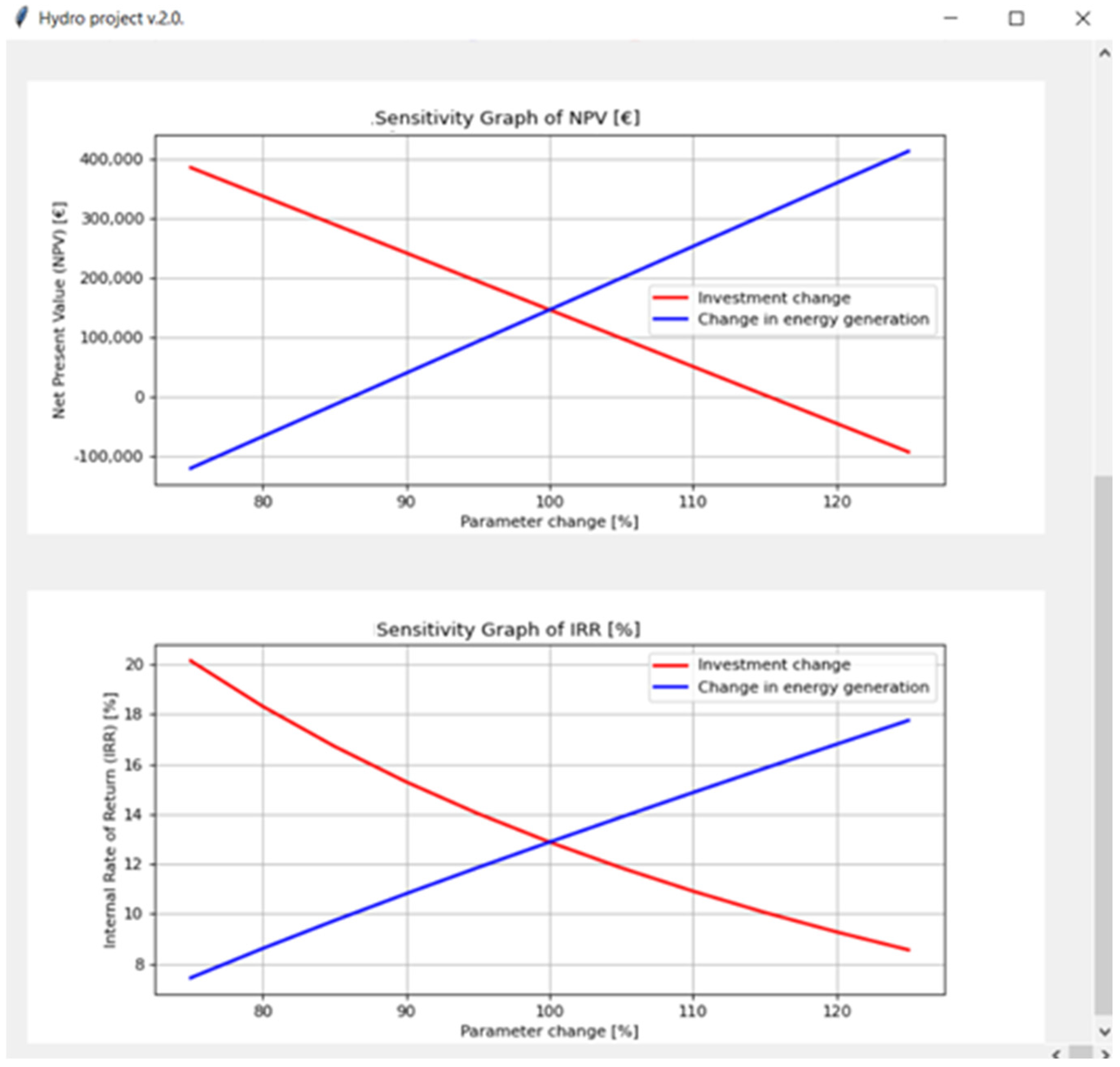
The sensitivity analysis of the plant produces results with a change in relevant plant parameters, for example, changes in income from the plant’s production or changes in the price of the plant’s investment. With this approach, the allowed economic margins of the plant are displayed, and the best and worst outcomes are shown in accordance with the given data. In the sensitivity analysis, for the sake of simplicity, the intervals of changes in income from electricity production and changes in the price of plant investment are predetermined and cannot be changed. The tool automatically displays the movement of the internal rate of return, the net present value, and the investment payback period in relation to the change of the previously mentioned input parameters that are changed.

The user interface of the sensitivity module is presented in Figure 19.

4. Software Verification

In order to determine the level of accuracy of the software, it is necessary to obtain an example on which the developed methodology and tool will be tested. The example with the corresponding calculation of technical and economic parameters is taken from [22], since it contains all the necessary parameters for input into the software. It is also possible to check and compare the obtained results with previously calculated data.

4.1. SHP Korana 1

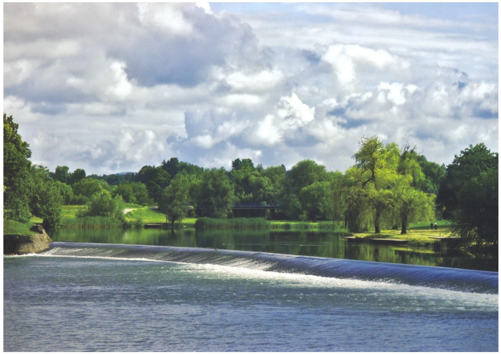
The SHP Korana 1 is located in the immediate vicinity of the Karlovac town on the Korana River, as shown in Figure 20 [22]. The Korana River flows out of the Plitvice Lakes, and its course is about 134.2 km long with a height drop of 425 m, with an average drop of 3.17‰ [22]. The Korana River has a smaller number of tributaries and a relatively stable flow of water and does not have a torrential character.

Historically speaking, a hydromill was built on the site in 1856 to be replaced by an industrial SHP during the Second World War, with the construction of a powerhouse and an overflow dam. With the aforementioned construction of the dam, a total head of almost 2.8 m is realized. Due to the weather factor, the dam had to be renovated in order to obtain satisfactory conditions again. This location has exceptional potential for the implementation of a SHP project at relatively low costs since the dam has been reconstructed and the foundations of the power plant building and the turbine chamber are in usable condition. According to [22], the plant type is run of the river with low-head.

4.2. Input Data

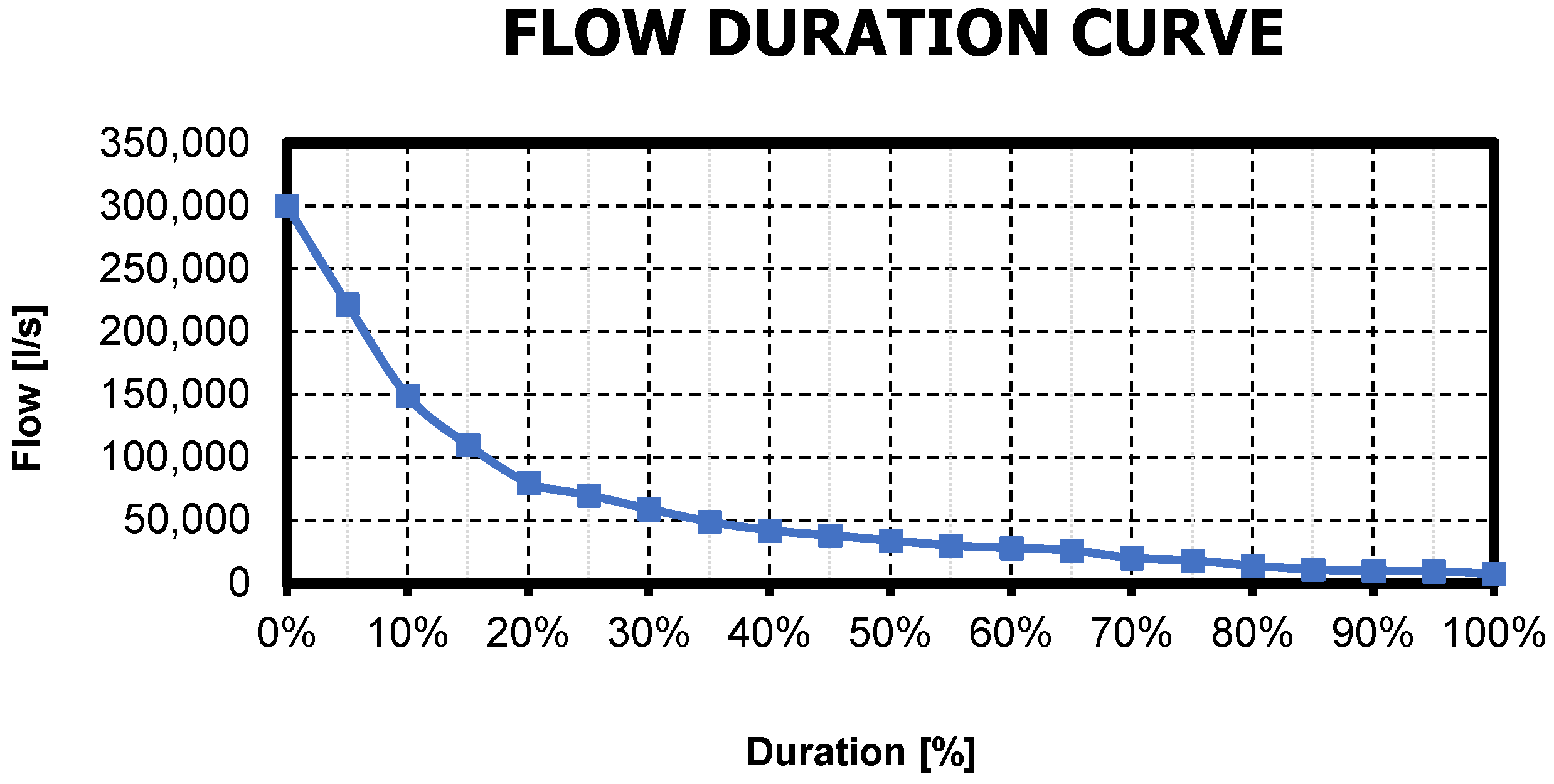
To evaluate the performance and accuracy of the results that will be obtained with the developed software, the same input data as in [22] were taken, including data on the flow duration curve, the design flow, and the available geodetic head. The selected location has a relatively stable flow with slower changes and is therefore suitable for exploiting the available hydropower potential. The measured and calculated flow values range from 300 to 7.5 m³, with an average flow value of 63.2 m³. The flow duration curve for the location is presented in Figure 21 [22].

Since this location involves the revitalization of the existing plant, and the parts that determine the maximum flow through the plant are in good condition, the maximum value of the design flow will not change, and the previously selected value of the design flow of the plant of 17 m³/s will be kept. The preliminary calculation will be made with the value of the geodetic head according to the data from [22], whose value is 2.7 m. This calculation will show the accuracy of the software and indicate any necessary corrections.

4.3. Results

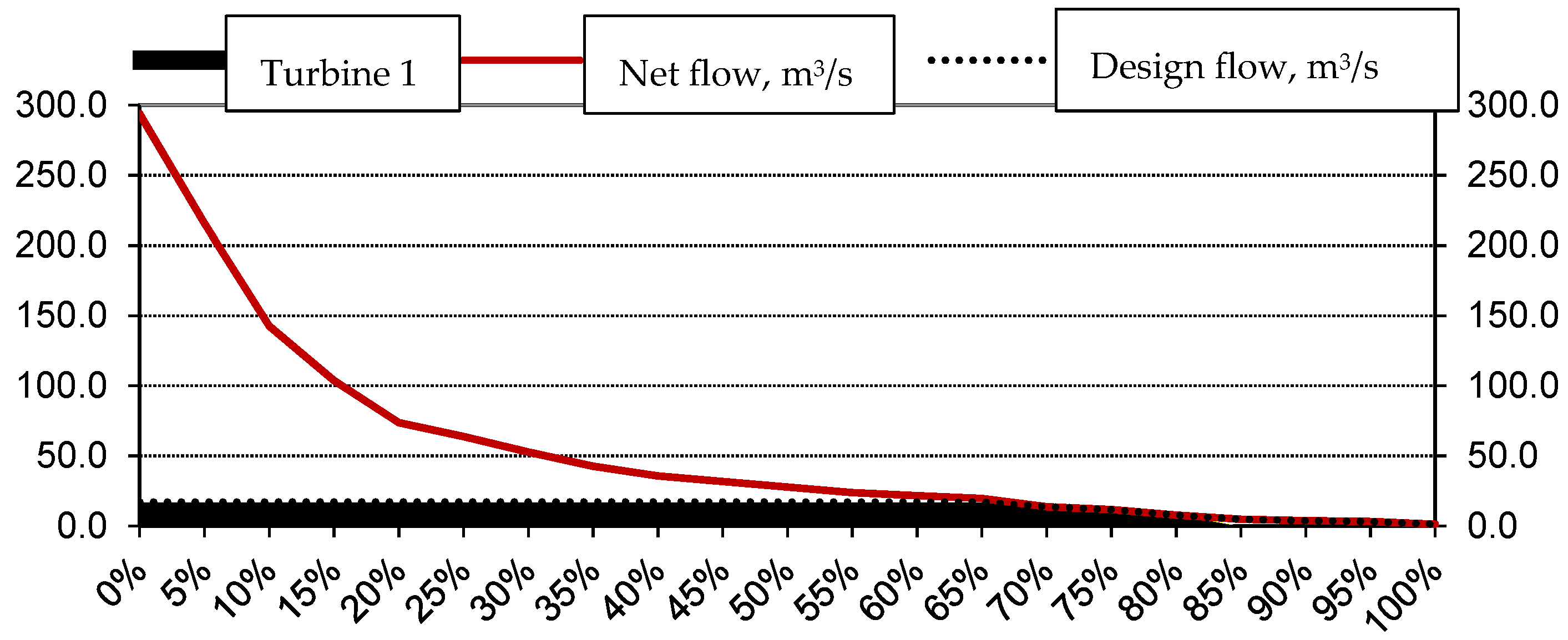
According to the given data, the tool recommended the selection of a VLH turbine; however, it is also possible to select a specific type of tubular turbine that would achieve satisfactory results. In accordance with the recommendation of the tool, a VLH turbine was chosen for the location, although according to the manufacturer’s data, it has lower efficiency in operation. A minimum flow value of 7.6 m³/s is selected for the specified turbine with a maximum turbine efficiency of almost 86%, as shown in Figure 22.

According to the given data, the value of the required maximum turbine power of 383 kW, the nominal plant power of 344 kW, and the average plant power of 312 kW is obtained. The total electricity produced according to the selected parameters of the plant is 2298 MWh. Visible differences in the calculation according to [22] and the developed software may be the result of different data on the efficiency of the turbine. The differences in the calculation results are shown in Table 3.

After calculating these parameters, it is possible to access the economic analysis of the planned plant. As mentioned earlier, it is about the revitalization of a SHP, and certain parts of the plant meet the conditions for a revitalized state, so they will not be changed. Therefore, the dam and the existing infrastructure do not need to be changed or revitalized. The necessary works include revitalization due to the change of turbine type and the construction of a new powerhouse.

The results show a certain difference in the calculation. In [22], it was stated that the exact information of the turbine manufacturer on the cost of turbine equipment and accompanying turbine equipment was obtained. Thus, the total cost calculated with the software is HRK 10.45 million (7.53450 HRK = 1.00 EUR), which differs by 2.5% from the cost obtained in [22].

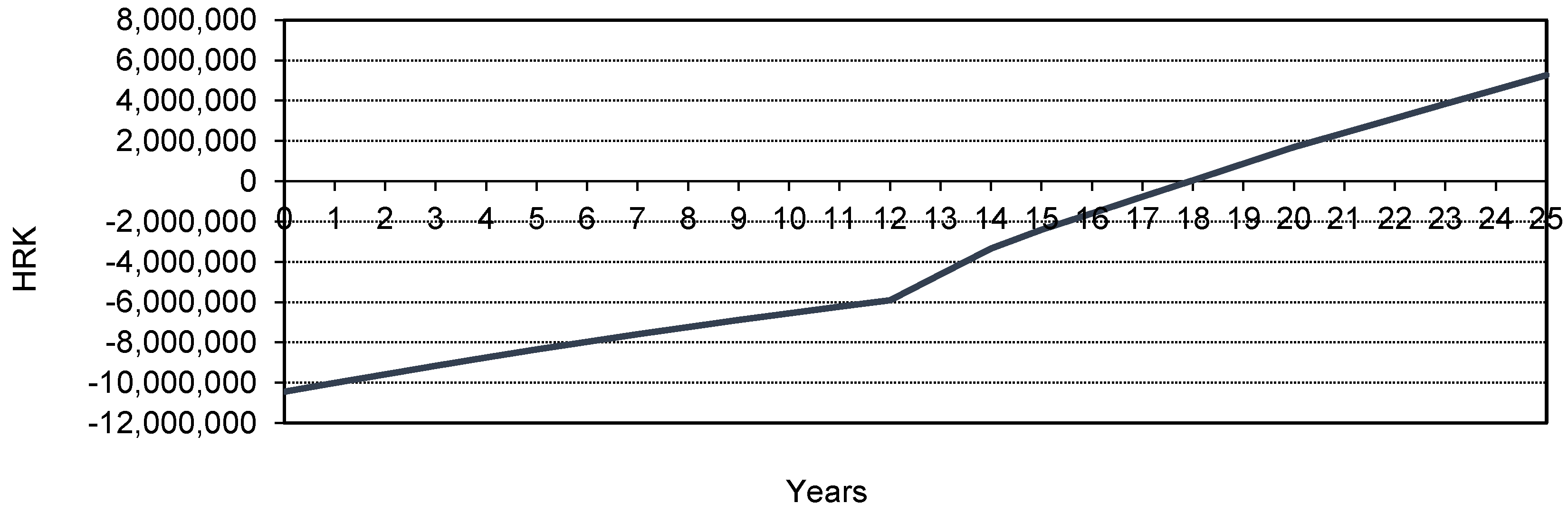
Further economic analysis, along with the calculated costs of maintenance, employees, and other material and non-material costs, shows that this type of plant revitalization is unprofitable. The investment return period is very long and amounts to almost 18 years with an internal investment return rate of 3%, as shown in Figure 23. Due to these results, it is concluded that it is necessary to select another type of turbine, preferably a tubular turbine that can work within the specified parameters. This would significantly reduce the cost of investment in an expensive VLH turbine.

5. Conclusions

Proper design of a SHP, based on the previously mentioned advanced technical solutions regarding the civil and electro-mechanical elements of SHP and environmental protection, using software tools for techno-economic analysis and effective legal/administrative procedures, should meet the basic principles of sustainable development, i.e., the investment should be designed and made in technical terms, in accordance with the applicable standards and regulations, provide certain economic benefits, and guarantee the absence of environmental hazards. The end product is a remarkably long-lasting, reliable, and potentially economical source of clean energy.

The development of a software for the techno-economic analysis of a SHP aims to improve the status of SHP projects and increase interest in this type of project. By presenting not only the potential technical outcomes, but also the economic parameters, the profitability of such plants in the considered cases will be indicated. Of course, the profitability of the plant will depend primarily on the available parameters of the geodetic head and flow at the location. This software provides the possibility of a quick calculation of the location parameters and lays a good foundation for a more detailed analysis of the plant in the further steps of planning appropriate solutions. By testing the software, certain differences in the results compared with previously performed calculations are noticeable, both in the technical part and in the economic part. However, it is necessary to take into account that the tool provides satisfactory estimates of investment costs in the economic part, since the calculation is based on general equations for each component of the plant. In both calculations, only the same flow duration curve and geodesic head were used as starting data.

The primary aim of this paper was to present a new software and the theoretical basics (equations) incorporated into it. The next step is more extensive simulations for different cases. The possibilities of upgrading the software will also be explored, primarily with additional equations in individual modules, in order to further expand its application possibilities.

Author Contributions

Conceptualization, Z.G. and Z.B.M.; methodology, Z.B.M., M.B. and Z.G.; software, Z.B.M. and M.B.; validation, Z.B.M.; formal analysis, Z.G.; investigation, Z.B.M., Z.G. and M.B.; resources, N.D.; data curation, Z.G.; writing—original draft preparation, Z.G.; writing—review and editing, Z.G. and N.D.; supervision, Z.G. and N.D.; project administration, N.D. All authors have read and agreed to the published version of the manuscript.

Funding

This research was funded by Croatian Science Foundation, grant number Project IP-2020-02-8568.

Data Availability Statement

Data supporting this study are included in the appendix.

Acknowledgments

This study has been fully supported by the Croatian Science Foundation under project IP-2020-02-8568.

Conflicts of Interest

The authors declare no conflict of interest.

Appendix A. Flow Duration Curve

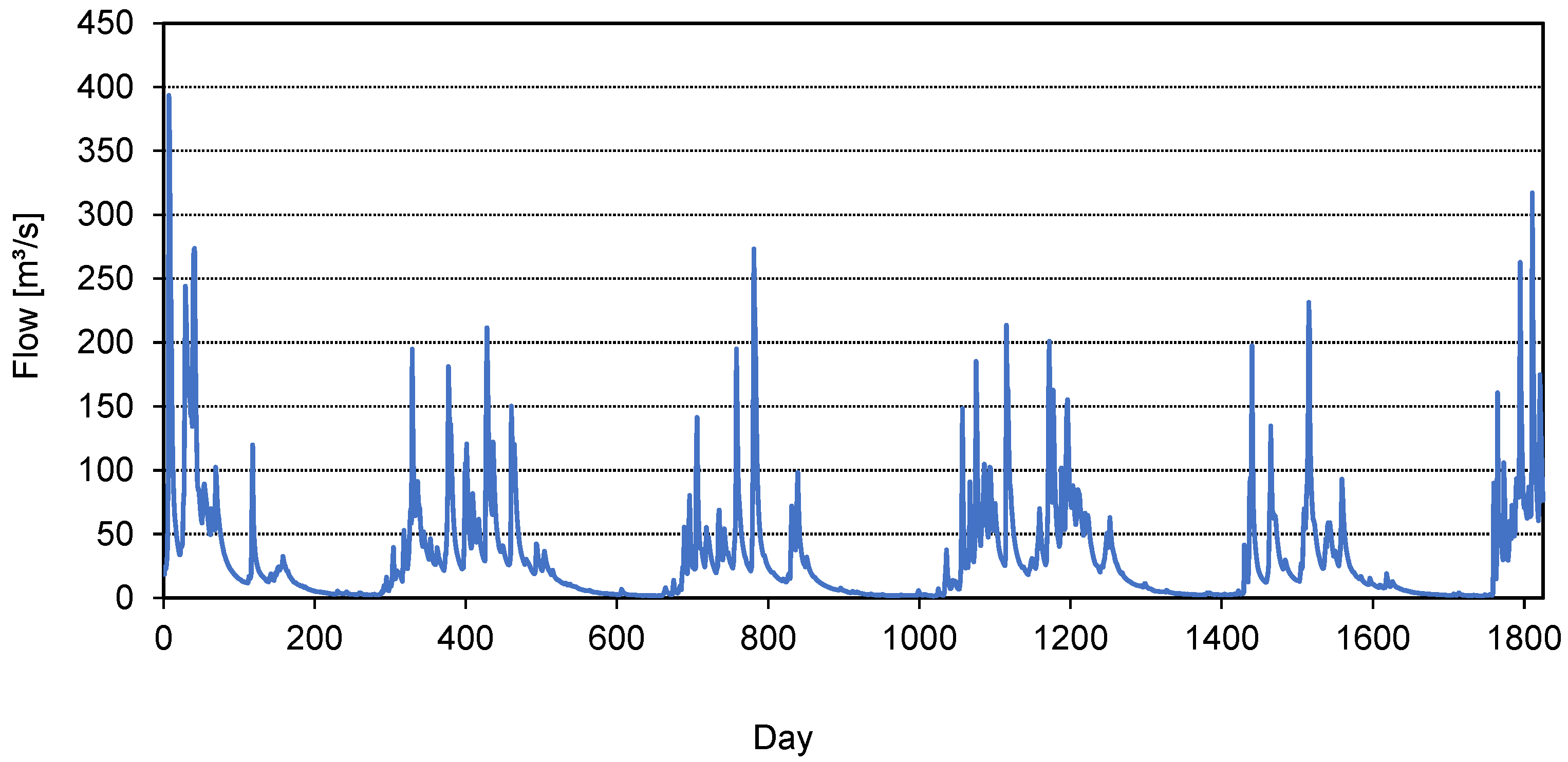
The flow duration curve (FDC) presents the average daily flow values related to the frequency of the occurrence of the same flow values during the observed time period. It is necessary to take a measurement period of flow as long as possible in order to obtain a more precise FDC. The measured flow values during the time period are represented by the hydrograph, as shown in Figure A1 [42].

Figure A1. An example of a hydrograph [42].

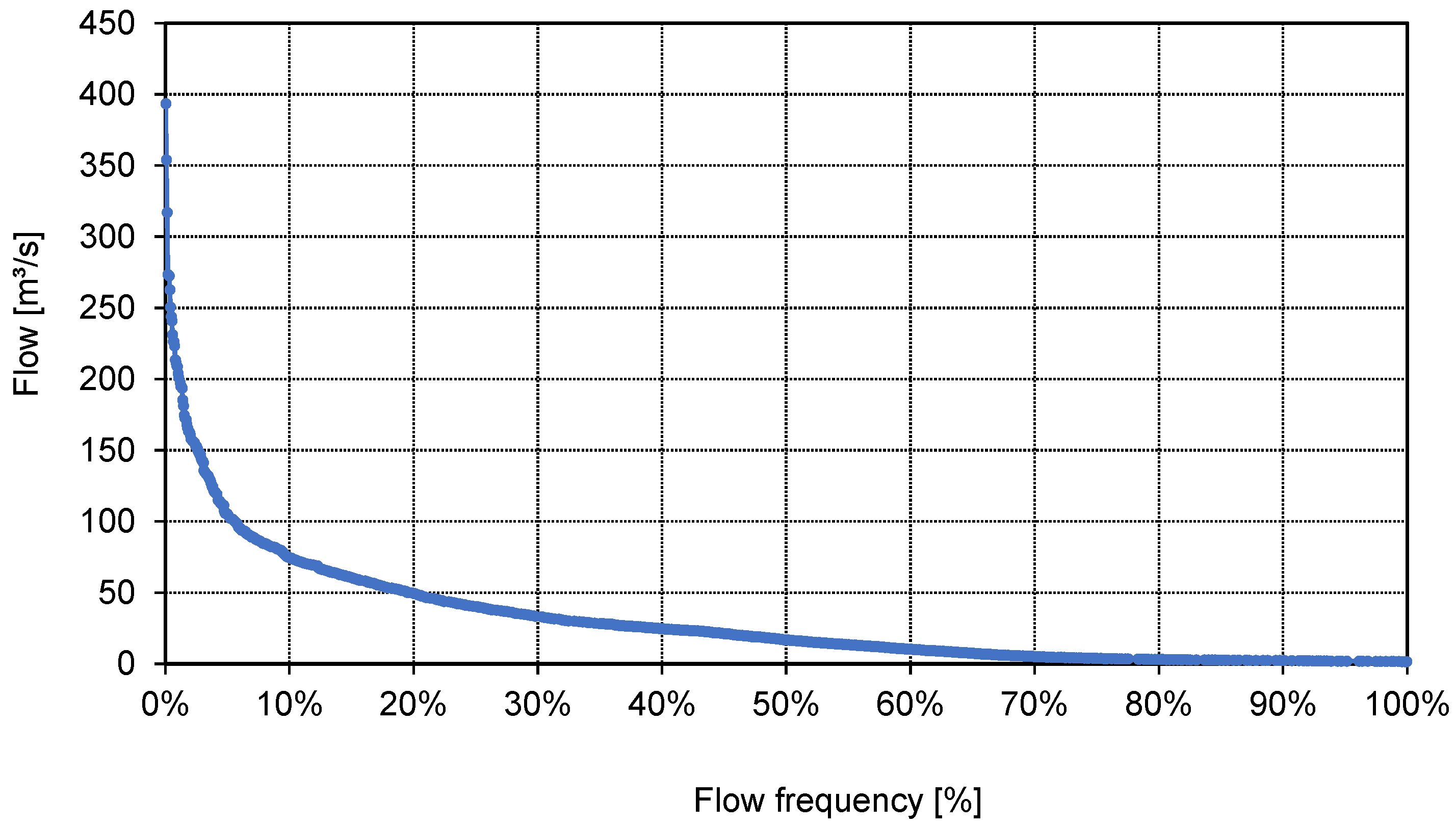
Then, the daily average flow values are classified by amount. The same daily average flow values have the ordinal number m and it is possible to calculate the probability of occurrence of a certain flow according to:

P = \frac{m}{(n + 1)} \times 100

(A1)

where n is the total number of collected daily values. The obtained FDC is presented in Figure A2 [42].

Figure A2. The flow duration curve [42].

The mean arithmetic value of the flow duration curve is calculated according to:

Q_{A V} = \frac{1}{n} \sum_{x = 0 %}^{x = 100 %} Q_{x %}

(A2)

where n is the number of items Q_x_% in the range 0–100% with a variable step of k = 5%.

Appendix B. Flow of the Ecological Minimum

In accordance with ecological requirements, it is not possible to completely divert the natural flow of water into a hydropower plant and return it in the downstream part of the river bed. By keeping a certain amount of water in the natural river bed, both the preservation of plant and fish species is ensured, and the requirements of other users of water resources are met [43].

The flow that should be passed through a natural river bed is called the ecological minimum or ecologically acceptable flow. More than 200 different calculation methods are in use to determine the mentioned flow.

Appendix B.1. Methods Based on Hydrological or Statistical Values

In methods based on hydrological or statistical values, the value of the ecological minimum depends on the statistical values of the flow of a certain water course, as shown in Table A1. These methods are easy to apply, assuming that the user has high-quality data, and enable the integration of natural deviations in the data.

However, it is important to note that with these methods it is possible to obtain too small flow values of the ecological minimum Q_ECO. Furthermore, methods based on hydrological or statistical values do not take into account the hydraulic parameters of the flow or the influence of tributaries when calculating the flow of the ecological minimum Q_ECO. These methods are not considered suitable for the case of mutual influence of two watercourses. Some of them are shown in Table A1 [43].

Table A1. Methods for the calculation of the ecological minimum based on hydrological or statistical values [43].

Method	Equation	Description
Method 10% of average flow value	$Q_{E C O} = 10 % \times Q_{A V}$ (A3)	The flow of the ecological minimum must be greater than 10% of the average value of the flow Q_AV. Attention should be paid to the fact that there is a temporal change in the flow of the ecological minimum Q_ECO. In order to meet the stated conditions, it is necessary to continuously measure the flow at different sections of the water flow, which makes this method demanding.
Lanser’s method	$Q_{E C O}^{M I N} = 5 % \times Q_{A V}$ (A4a) $Q_{E C O}^{M A X} = 10 % \times Q_{A V}$ (A4b)	The calculation of the flow of the ecological minimum is set in a certain interval, more precisely between 5 and 10% of the mean value of the flow Q_AV.
Jager’s method	$Q_{E C O} = 15 % \times Q_{A V}$ (A5)	It suggests considering the importance of the fish population in the watercourse; the flow of the ecological minimum is calculated as 15% of the mean value of the flow Q_AV.
The Montana method	$Q_{E C O} = 40 - 60 % \times Q_{A V}$ (A6a) $Q_{E C O} = 10 % \times Q_{A V}$ (A6b)	It takes into account the economic importance of fishing in a certain watercourse. In case of a high economic importance of fishing, Q_ECO is calculated for an interval 40–60% of the average flow Q_AV, while in case of a small economic importance of fishing, Q_ECO is calculated as 10% of the Q_AV.
Steinbach’s method	$Q_{E C O} = Q_{A V, m i n}$ (A7)	Q_ECO is calculated in such a way that it must be equal to the minimum average flow Q_AV,min, taking into account a longer period of time and the seasonal distribution, i.e., the division into summer and winter periods.
Rheinland-Pfalz method	$Q_{E C O}^{M I N} = 20 % \times Q_{A V, m i n}$ (A8a) $Q_{E C O}^{M A X} = 50 % \times Q_{A V, m i n}$ (A8b)	Calculation of Q_ECO is set in a certain interval, more precisely between 20 and 50% of the minimum average flow value Q_AV,min.
Alarm limit value method	$Q_{E C O} = 20 % \times Q_{300}$ (A9)	It imposes the calculation of Q_ECO as the flow needed to ensure the ecological requirements of the watercourse in the amount of 20% of the flow that occurs at least 300 days a year Q₃₀₀.
Sawall and Simon method	$Q_{E C O}^{M I N} = 7 % \times Q_{A V, A V G}^{m i n}$ (A10a) $Q_{E C O}^{M A X} = Q_{A V, A V G}^{m i n}$ (A10b)	Q_ECO is calculated in the interval of 7–100% of the minimum average flow in the month of August $Q_{A V, A U G}^{m i n}$ , taking into account the longer time period of flow measurement.
The method of fitting with the flow duration curve (Fitting to FDC)	$Q_{E C O} = \frac{Q_{84 %, S} + Q_{84 %, K}}{2}$ (A11)	It prescribes Q_ECO in such a way that the amount of flow Q_ECO is calculated as the mean value of the difference of the flow between dry and rainy years which is present for more than 84% of the duration of one year. The differences between the flow duration curves for dry and rainy years are particularly pronounced in some geographical areas; therefore, it is possible to observe significant differences in flow values Q_84%. Q_84%,S represents the value of the flow that is present for 84% of the duration of the dry year, and Q_84%,K represents the value of the flow that is present for 84% of the duration of the rainy year.

Appendix B.2. Comparative Analysis of Methods Based on Hydrological Values

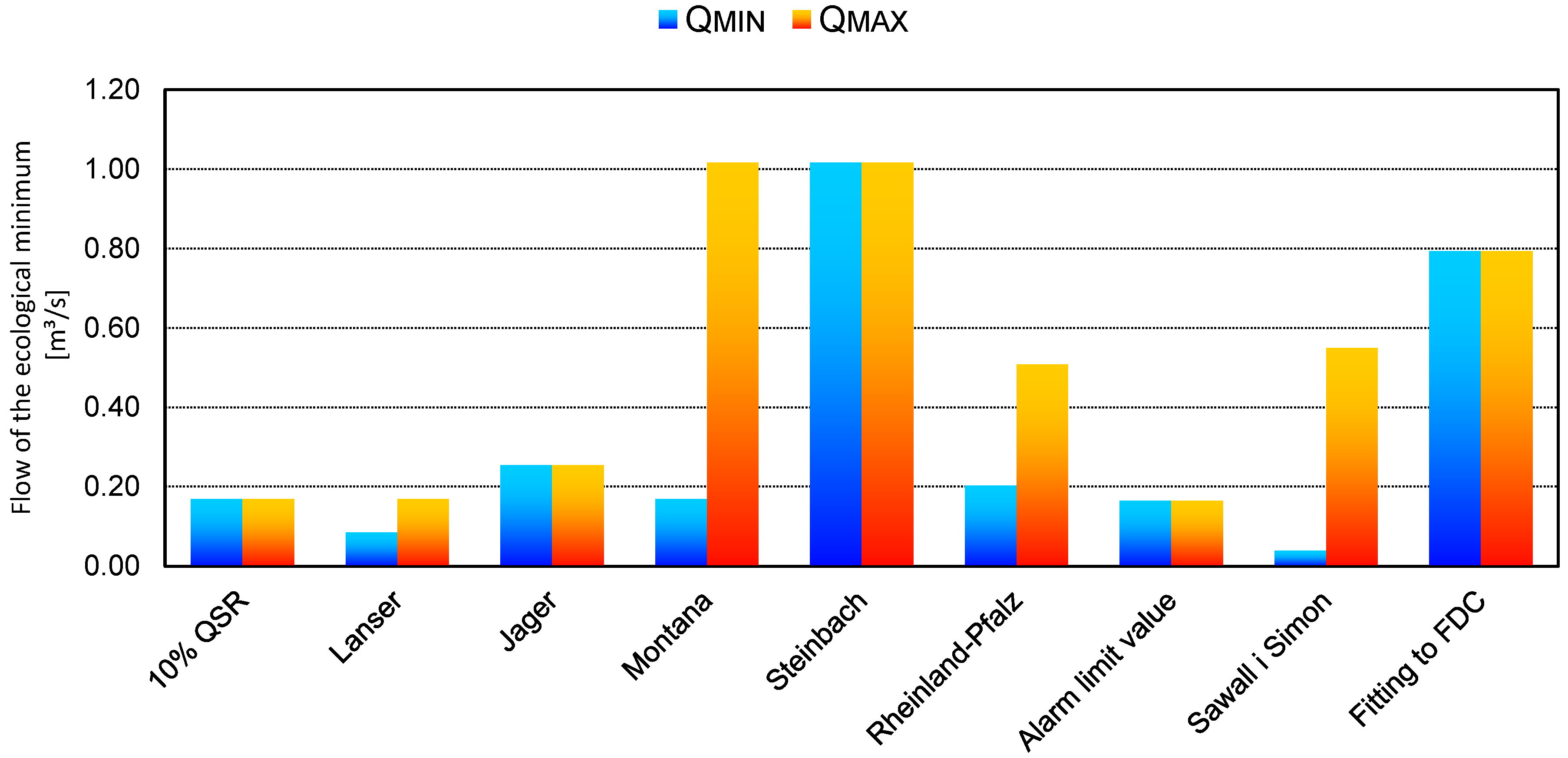
A comparative analysis of methods based on hydrological or statistical parameters is made to show the requirements of each method on the flow value of the ecological minimum. For analysis, a watercourse is taken, for which the corresponding FDC is presented in Figure A2. Results of comparative analysis are presented in Figure A3.

Figure A3. Minimum values of ecological flow for the mentioned calculation methods.

It is evident that Steinbach’s method has the highest requirements related to the flow value of the ecological minimum, where a high value of the flow of the ecological minimum is necessarily imposed. Along with the Steinbach method, the Montana method also has the same value of the maximum flow of the ecological minimum. The Sawall and Simon method, the Montana method, and the Rheinland–Pfalz method have a fairly large interval of the limits of the minimum and maximum flow values of the ecological minimum, which enables the user to select values within the interval and optimal design in accordance with energy, economic, and environmental requirements. The Sawall and Simon method has the lowest calculated value of the lower flow limit of the ecological minimum.

Appendix B.3. Methods Based on Water Depth and Velocity

These methods of determining the flow of the ecological minimum include the measurement of the flow value, more precisely, the velocity of the water flow and the depth of the water. Some of them are shown in Table A2 [43].

Table A2. Methods for calculation of the ecological minimum based on water depth and velocity [43].

Method	Equation	Description
Steiermark method	$Q_{E C O}^{M I N} = v^{M I N} \times h_{w} \times b_{U S E}$ (A12a) $Q_{E C O}^{M A X} = v^{M A X} \times h_{w} \times b_{U S E}$ (A12b)	The flow rate and water depth are measured in the area between the partition and the drainage system. The set conditions determine that: the water velocity in case of residual flow must not fall below the level of 0.3–0.5 m/s; the minimum water depth must be greater than 0.1 m. v^MIN and v^MAX are the minimum and maximum inlet velocity, h_w is the minimum water depth, and b_USE is the useful water depth. This method also provides an interval of values within which the flow value of the ecological minimum must change. The results obtained are within the limits determined by the given input speeds since they are the only variables in the above equations. Choosing the correct value in the interval depends on the user.
Oregon method	$Q_{E C O}^{M I N} = v^{M I N} \times h_{w}^{M I N} \times b_{U S E}$ (A13a) $Q_{E C O}^{M A X} = v^{M A X} \times h_{w}^{M A X} \times b_{U S E}$ (A13b)	The requirements of the Oregon method differ significantly from the Steiermark method, with measurements being made on the depleted portion of the watercourse. Relevant conditions are also related to the inlet velocity of the current within the limits of 1.2–2.4 m/s, and the water depth within the limits of 0.12–0.24 m. v^MIN and v^MAX are the minimum and maximum inlet velocity, $h_{w}^{M I N}$ and $h_{w}^{M A X}$ are the minimum and maximum water depth in the exhausted part of the water flow, and b_USE is the useful water depth
Oberösterreich method	$Q_{E C O} = v \times h_{w} \times b_{U S E}$ (A14)	It imposes a condition only on the water depth in the exhausted part of the water course, which is 0.2 m.

Appendix C. Net Flow Calculation

Net flow is calculated based on the flow value minus the ecological minimum flow value for each item in the flow duration curve:

Q_{N E T, x %} = Q_{x %} - Q_{E C O}

(A15)

where

Q_{N E T, x %}

indicates the net flow for the defined step (0–100),

Q_{x %}

the flow value according to the data for the flow duration curve, and

Q_{E C O}

the previously calculated flow of the ecological minimum. After obtaining the results, it is possible to design the net flow duration curve.

Calculation of the Flow of a SHP

By calculating the flow of a SHP, the value of the design flow is determined, which is used in the further steps of the calculation to obtain the final target parameters. Defining the design flow directly influences the selection of the turbine for the planned plant, where it is necessary to take into account other influential parameters such as the available geodetic head.

The designed flow can be determined in two ways:

By direct calculation from the given data in the flow curve;
By manually entering the desired value of the designed flow.

Appendix D. Net Head Calculation

When considering the project of a SHP, it is certainly necessary to take into account flow losses in the supply structures in order to correctly dimension the turbine. Flow losses occur due to the roughness of the structure, changes in the flow direction, and other irregularities. In the following, the methodology for calculating flow losses for pipelines and channels with an open water face are presented.

Total head losses are calculated according to:

h_{N E T} = h_{G E O} - h_{P I P (C H A)}

(A16)

Appendix D.1. Flow Losses in Pipelines

Flow losses in pipelines are to a certain extent greater than losses in open channels. Flow losses are divided into line and local losses to obtain the total amount of losses. Table A3 presents equations for the calculation of flow losses in pipelines [44].

Table A3. Equations for the calculation of flow losses in pipelines [44].

Type of Loss	Equation	Description
Line losses	$h_{G H} = 10.29 \times L_{P I P} \times \frac{Q_{D E S}^{2}}{K_{s} \times D_{P I P}}$ (A17)	$L_{P I P}$ is the total length of the pipeline, $Q_{D E S}$ is the designed flow, $K_{s}$ Strickler’s roughness, and $D_{P I P}$ is the selected diameter of the pipeline calculated according to the designed flow and the given speed of water flow in the pipeline.
Local losses	$h_{G L} = α \times \frac{v_{C O R}^{2}}{2 g}$ (A18)	$v_{C O R}$ is the corrected speed of water flow in the pipeline calculated as a function of the selected diameter of the pipeline $v_{C O R} = f (D_{P I P})$ , α is the size factor of local losses, and g is the acceleration of the gravitational force.
The total losses	$h_{P I P} = h_{G H} + h_{G L}$ (A19)	It subtracts from the total realizable geodetic head.

Appendix D.2. Flow Losses in Open Channels

The procedure for determining flow losses in open channels [45] is significantly different from the calculation of flow losses in pipelines. Table A4 presents equations for the calculation of flow losses in open channels.

Table A4. Equations for the calculation of flow losses in open channels [45].

Type of Loss	Equation	Description
Chézy-Manning equation	$Q = \frac{A \times R_{h}^{2 / 3} \times S_{0}^{1 / 2}}{n}$ (A20)	A is the cross-sectional area of the channel, S₀ is the slope of the channel, n is the Guckler–Manning coefficient, and R_h is the hydraulic radius of the channel. R_h is a measure of the flow efficiency in the channel depending on the cross-section of the channel.
The hydraulic radius	$R_{h} = \frac{A}{P_{L}}$ (A21)	P_L is the “wetted perimeter” of the channel under consideration. It is necessary to achieve the largest possible hydraulic radius of the channel in order to achieve greater efficiency. P_L is the sum of the length of the submerged parts of the individual sides of the channel.
Line losses in channels with an open water face	$y_{1} + \frac{v_{1}^{2}}{2 g} + S_{0} \times L_{C H A} = y_{2} + \frac{v_{2}^{2}}{2 g} + h_{L}$ , (A22) with y₁ = y₂ = const. and v₁ = v₂ = const.: $S_{0} \times l = h_{L}$ ; $S_{0} = \frac{h_{L}}{l}$ ; (A23) $Q = \frac{A \times {(\frac{A}{P_{L}})}^{2 / 3} \times {(\frac{h_{L}}{l})}^{1 / 2}}{n};$ (A24) $h_{L} = \frac{Q^{2} {\times n}^{2} \times l \times P_{L}^{4 / 3}}{A^{10 / 3}};$ (A25) $n = \frac{1}{K_{S}};$ (A26) $h_{L} = \frac{Q^{2} \cdot l \cdot P_{L}^{4 / 3}}{A^{10 / 3} \cdot K_{S}^{2}}$ (A27)	S₀ is the slope of the channel, L_CHA is the length of the channel, and h_L is the flow loss in the channel, n—the Gauckler–Manning coefficient. For a square cross-section: $P_{L} = \frac{2 \frac{Q}{v_{C H A}}}{{(w}_{K} \times h_{K})} \times h_{K} + w_{K},$ v_CHA is the designed velocity of flow in the channel, h_K is the height of the lateral sides of the channel, and w_K is the length of the lower side of the channel. For a circular cross-section: $P_{L} = D_{C H A} \times π \times \frac{\frac{Q}{v_{C H A}}}{(\frac{D_{C H A}^{2} \times π}{4})},$ D_CHA is the diameter of the channel calculated according to the designed flow and the designed velocity in the channel. For a trapezoidal cross-section: $P_{L} = \frac{2 \cos α_{D, K} \times l_{k} \frac{\frac{Q}{v_{C H A}}}{(w_{D, K} + \sin (α_{D, K} - 90) l_{k}) (\cos (α_{D, K} - 90) l_{k})}}{\cos (α_{D, K} - 90) + w_{D, K}},$ $α_{D, K}$ is the angle between the side of the trapezoid $l_{k}$ and the lower base of the trapezoid $w_{D, K}$ .

The minimum flow through the turbine

Q_{M I N, T}

is the information provided by the turbine manufacturer, and is calculated according to:

Q_{M I N, T} = φ \times Q_{D E S}

(A28)

Appendix E. Calculation of SHP Parameters

In order to estimate SHP parameters, which are obtained from the input and calculated data on the net head and the design flow, it is necessary to set up calculation expressions that will obtain the power of the plant and show other parameters of the plant in operation.

The maximum power of the plant is calculated according to:

P_{M A X} = Q_{D E S} \times g \times h_{N E T} \times η_{T}

(A29)

where

Q_{D E S}

is the design flow of a SHP, g is the acceleration of the gravitational force,

h_{N E T}

is the net head, and

η_{T}

is the maximum efficiency of the selected turbine for the design flow. Additionally, it is necessary to calculate the nominal power of the plant

P_{N O M}

according to:

P_{N O M} = 0.9 P_{M A X}

(A30)

The electricity produced at each single moment of the flow duration and for each individual turbine is calculated according to:

E_{i %, T} = t_{W O R} \times η_{G} \times η_{T R} \times η_{R} \times P_{T} \times (Q_{x %} - Q_{M I N, T})

(A31)

where

t_{W O R}

is the operating time of the turbine (8760 h),

η_{G}

generator efficiency,

η_{T R}

transformer efficiency,

η_{R}

transmission efficiency,

P_{T}

turbine,

Q_{x %}

flow at a particular moment of flow duration, and

Q_{M I N, T}

minimum flow through the turbine.

The total electricity produced in the year

E_{Y E A}

is obtained from the expression:

E_{Y E A} = (1 - t_{%}) \sum_{i = 1}^{i = 0} E_{i %, T}

(A32)

where t_% is the percentage of time per year that the plant is out of service.

Appendix F. Investment Calculation

The calculation of the investment in a SHP project requires an estimation of the costs of all components based on empirical equations or curves obtained from the collection of data on real investments. The calculation of the investment for a SHP needs to be connected with the technical part of the calculation in order to obtain functional dependencies of the size of individual components and costs as a result of given parameters. The accuracy of the results is difficult to verify since each plant is a separate case where costs for similar parameters can differ significantly. The cost of off-the-shelf parts can also be problematic since equipment manufacturers are in most cases unwilling to give away the actual cost of the equipment to be used. The problem also arises due to the relatively large market where prices vary significantly; therefore, the total investment may vary depending on the manufacturer of the required equipment. The empirical equations for calculation of the cost of individual components of a SHP are given in Table A5 [44,45,46,47].

Table A5. The empirical equations for calculation of cost of individual components of a SHP [44,45,46,47].

Component		Equation	Description
Dam		$C_{D A} = a_{0}$ $, Q < 0.1 {[m}^{3} / s]$ (A33a)	Coefficients a₀–a₃ are defined in accordance with the associated data and differ for each of the specified flow intervals. Higher order equations are applied for other flows.
		$C_{D A} = a_{2} \times Q^{2} + a_{1} \times Q + a_{0},$ $Q < 0.1 {[m}^{3} / s]$ (A33b)
		$C_{D A} = a_{3} \times Q^{3} + a_{2} \times Q^{2} + a_{1} \times Q + a_{0},$ $1 \leq Q < 10 {[m}^{3} / s]$ (A33c)
Catchment structure		$C_{C S} = a_{1} \times A_{C S} + a_{0}$ (A34)	The coefficients a₁ and a₀ differ for different flows and depend on the application of a particular type of intake, and A_CS is the area of the intake determined on the basis of the given flow rate and flow speed in the intake.
The power plant building		$C_{B U} = a_{1} \times Q^{a_{0}}$ (A35)	The coefficients a₁ and a₀ are different for different flows.
Turbinetype	Pelton	$C_{T U} = a_{2} \times Q^{2} + a_{1} \times Q + a_{0}$ , $< 500 k W$ ; (A36a) $C_{T U} = a_{1} \times Q^{a_{0}}$ , $> 500 k W$ (A36b)	The classification of coefficients a₀–a₂ is according to the calculated geodetic head.
	Francis	$C_{T U} = a_{1} \times Q^{a_{0}}$ , $< 500 k W$ ; (A37a) $C_{T U} = a_{1} \times \ln Q + a_{0}$ , $> 500 k W$ (A37b)	The classification of coefficients a₀–a₁ is according to the calculated geodetic head.
	Kaplan	$C_{T U} = a_{1} \times Q^{a_{0}}$ (A38)	The classification of coefficients a₀–a₁ is according to the calculated geodetic head.
	Cross flow, DIVE, Turgo, VLH	$C_{T U} = a_{2} \times P^{a_{1}} \times H^{a_{0}}$ (A39)	The coefficients a₀–a₂ change depending on the number of installed turbines, P is the installed power of the turbine, and H is the calculated geodetic head.
Electric generator		$C_{G E} = a_{1} \times P^{a_{0}}$ (A40)	The price of the electric generator is expressed as a function of the installed power of the turbine. The coefficients a₀–a₁ are the same for all cases; however, with a turbine power of less than 500 kW, it is taken into account that the cost of the generator is included in the cost of the turbine, and it is omitted from the cost of the generator.
Transformer		$C_{T R} = a_{1} \times P + a_{0}$ (A41)	The coefficients a₀–a₁ depend on the installed power of the turbine and are divided into three classes.
Pipelines		$C_{P I P} = a_{1} \times D + a_{0}$ (A42)	The coefficients a₀–a₂ depend on the installed power of the turbine.
Canals		$C_{C H A} = a_{2} \times P^{a_{1}} \times H^{a_{0}} \times x$ (A43)
Other mechanical and electrical equipment		$C_{O O} = a_{2} \times P^{a_{1}} \times H^{a_{0}}$ (A44)	The coefficients a₀–a₁ depend on the number of installed turbines. The final price depends on the number of turbines installed, as well as on the power of the turbines and the calculated geodetic head.
Cost of work		$C_{R A} = (C_{D A} + C_{C S} + C_{B U} + C_{T U} + C_{G E} + C_{T R} + C_{P I P / C H A} + C_{O O}) \times 10 %$ (A45)
Cost of services and design		$C_{O S T} = (C_{D A} + C_{C S} + C_{B U} + C_{T U} + C_{G E} + C_{T R} + C_{P I P / C H A} + C_{O O}) \times 3 % (A 46)$

Appendix G. Calculation of Economic and Financial Parameters

In order to evaluate projects, it is necessary to lay valid foundations for calculating the economic parameters of the project in accordance with the given technical data and data on the total costs of the plant. The financial and economic assessment of the project is of great importance when it comes to making the final decision on the implementation of the project. In accordance with the requirements, below is an overview of the methodology used for the financial and economic evaluation of the project.

The income from the sale of produced electricity is the only income generated by the plant, and represents the product of the total energy produced during the calendar year and the purchase price of electricity in accordance with the tariff system for the production of energy from renewable energy sources for the duration of the contract on the purchase of electricity from renewable sources:

R_{Y E A, P T} = E_{Y E A} \times C_{R E S}

(A47)

After the incentive tariff expires, it represents the product of the total energy produced during the calendar year and the purchase price of electricity (EUR/kWh) in accordance with market rules:

R_{Y E A} = E_{Y E A} \times C_{N O R M A L}

(A48)

Since the cost of the plant is high in most cases, it is difficult to obtain financing entirely from one’s own resources, and the use of loans is required. With such projects, there is a requirement to participate in financing from own funds in certain amounts. Accordingly, the required amount of the loan is the difference between the total amount of the investment and the amount that needs to be settled with own funds:

T_{L O} = I_{T O T} - I_{O F}

(A49)

Equal annual loan installments are calculated from the total required loan amount according to:

A_{L O} = i \frac{{(1 + i)}^{n_{L O}}}{({(1 + i)}^{n_{L O}} - 1)}

(A50)

where i is the loan interest rate, n_LO is the number of periods, and A_LO is the calculated annual annuity.

In order to obtain the relevant parameters for the project evaluation, it is necessary to provide an overview of plant costs in the balance sheet, which includes maintenance costs T_OD, insurance T_OS, employes T_Z, plant costs T_PO, other material costs T_MAT, and other costs T_OST.

Depreciation is the process of reducing the value of the company’s assets (with the simultaneous transfer of that value to the corresponding accounts receivable) and is calculated annually according to the procedure provided for in the corresponding legal framework. In financial analyses, the linear method of depreciation is most often used, which determines equal amounts of depreciation costs. Accordingly, the annual depreciation expense is calculated according to:

T_{A M} = \frac{T_{G R}}{n_{P E R}},

(A51)

where T_GR is the cost of a specific group (equipment, works, etc.), and n_PER is the number of periods during which depreciation is calculated for a particular group.

Total costs take into account all previously mentioned cost groups:

T_{U K} = T_{O D} + T_{O S} + T_{Z} + T_{P O} + T_{M A T} + T_{O S T}

(A52)

The difference between total costs and total revenues represents the profit of the company (plant) that will be realized during the year:

I_{P R O} = R_{Y E A} - T_{U K}

(A53)

Profit tax is charged on the realized profit, in accordance with the legal framework. The tax base for income tax represents the difference between realized profit, depreciation costs, and loan interest:

I_{P O} = I_{P R O} - T_{A M} - A_{L O}

(A54)

Based on the calculated tax base, the profit tax is calculated according to the equation:

I_{P D} = I_{P O} \times 20 %

(A55)

By reducing the realized profit for the tax base and the cost of paying the annuity of the loan, the net amount of profit is obtained, which is used to calculate the parameters necessary for the evaluation of the project. The internal rate of return of an investment is used to assess profitability and does not include the influence of interest rates or inflation in its calculation. The internal rate of return of the investment is the discount rate at which the net present value of the costs (negative cash flows) of the investment is equal to the net present value of the positive cash flows of the investment. As soon as the internal rate of return of a certain project is higher, the investment is more desirable, and the probability of its implementation is higher. Basically, any project whose internal rate of return is greater than the cost of capital is profitable and recommended for implementation. The internal rate of return is calculated according to:

N P V = \sum_{n = 0}^{N} \frac{C_{n}}{{(1 + r)}^{n}}

(A56)

where NPV is the net present value of the project, N is the total considered number of periods, n is the considered period, C_n is the cash flow in the considered period, and r is the internal rate of return on the investment. Additionally, the basic analysis needs to show the net present value of the project itself, and a simple investment return period that shows the time period during which a specific investment will pay off, taking into account the net amounts of cash flows. According to the statement, the simple investment return period is calculated according to:

J P P = \frac{I_{T O T}}{\sum_{0}^{n} I_{N E T}}

(A57)

where I_NET are realized cash flows during the period, and n is the number of periods that need to be taken into account.

References

Liu, D.; Liu, H.; Wang, X.; Kremere, E. (Eds.) World Small Hydropower Development Report; United Nations Industrial Development Organization: Viena, Austria; International Center on Small Hydro Power: Hangzhou, China, 2019; Available online: www.smallhydroworld.org (accessed on 1 February 2021).
Paris Climate Agreement. Available online: https://unfccc.int/sites/default/files/english_paris_agreement.pdf (accessed on 1 February 2021).
Adhikary, P.; Kundu, S. Small Hydropower Project: Standard Practices. Int. J. Eng. Sci. Adv. Technol. 2014, 4, 241–247. [Google Scholar]
Dragu, C.; Sels, T.; Belmans, R. Small Hydro Power—State of the Art and Applications; K.U. Leuven: Leuven, Belgium, 2001. [Google Scholar]
International Hydropower Association (IHA). Congress Draft of the San José Declaration on Sustainable Hydropower. In Proceedings of the World Hydropower Congress, San José, CA, USA, 7–24 September 2021. [Google Scholar]
Walczak, N. Operational Evaluation of a Small Hydropower Plant in the Context of Sustainable Development. Water 2018, 10, 1114. [Google Scholar] [CrossRef]
Iqbal, M.; Azam, M.; Naeem, M.; Khwaja, A.S.; Anpalagan, A. Optimization classification, algorithms and tools for renewable energy: A review. Renew. Sustain. Energy Rev. 2014, 39, 640–654. [Google Scholar] [CrossRef]
Zhang, Y.; Ma, H.; Zhao, S. Assessment of hydropower sustainability: Review and modeling. J. Clean. Prod. 2021, 321, 128898. [Google Scholar] [CrossRef]
Ayik, A.; Ijumba, N.; Kabiri, C.; Goffin, P. Preliminary assessment of small hydropower potential using the Soil and Water Assessment Tool model: A case study of Central Equatoria State, South Sudan. Energy Rep. 2023, 9, 2229–2246. [Google Scholar] [CrossRef]
Quaranta, E.; Muntean, S. Wasted and excess energy in the hydropower sector: A European assessment of tailrace hydrokinetic potential, degassing-methane capture and waste-heat recovery. Appl. Energy 2023, 329, 120213. [Google Scholar] [CrossRef]
Punys, P.; Dumbrauskas, A.; Kvaraciejus, A.; Vyciene, G. Tools for Small Hydropower Plant Resource Planning and Development: A Review of Technology and Applications. Energies 2011, 4, 1258–1277. [Google Scholar] [CrossRef]
Kelly-Richardsa, S.; Silber-Coatsa, N.; Crootofa, A.; Tecklinb, D.; Bauera, C. Governing the transition to renewable energy: A review of impacts and policy issues in the small hydropower boom. Energy Policy 2017, 101, 251–264. [Google Scholar] [CrossRef]
Couto, T.B.A.; Olden, J.D. Global proliferation of small hydropower plants—Science and policy. Front Ecol. Environ. 2018, 16, 91–100. [Google Scholar] [CrossRef]
Agarwal, S.S.; Kansal, M.L. Risk based initial cost assessment while planning a hydropower project. Energy Strategy Rev. 2020, 31, 100517. [Google Scholar] [CrossRef]
Alp, A.; Akyüz, A.; Kucukali, S. Ecological impact scorecard of small hydropower plants in operation: An integrated approach. Renew. Energy 2019, 12, 3446. [Google Scholar] [CrossRef]
Diaz, P.; Adler, C.; Patt, A. Do stakeholders’ perspectives on renewable energy infrastructure pose a risk to energy policy implementation? A case of a hydropower plant in Switzerland. Energy Policy 2017, 108, 21–28. [Google Scholar] [CrossRef]
Ullah, K.; Razza, M.S.; Mirza, F.M. Barriers to hydro-power resource utilization in Pakistan: A mixed approach. Energy Policy 2019, 132, 723–735. [Google Scholar] [CrossRef]
Adu, D.; Zhang, J.; Fang, Y.; Suoming, L.; Darko, R.O. A Case Study of Status and Potential of Small Hydro-Power Plants in Southern African Development Community. Energy Procedia 2017, 14, 352–359. [Google Scholar] [CrossRef]
Venus, T.E.; Hinzmann, M.; Bakken, T.H.; Gerdes, H.; Godinho, F.N.; Hansen, B.; Pinheiro, A.; Sauer, J. The public’s perception of run-of-the-river hydropower across Europe. Energy Policy 2020, 140, 111422. [Google Scholar] [CrossRef]
Sammartano, V.; Liuzzo, L.; Freni, G. Identification of potential locations for run-of-river hydropower plants using a GIS-based procedure. Energies 2019, 12, 3446. [Google Scholar] [CrossRef]
Francfort, J.E.; Matthews, S.D.; Rinehart, B.N. Uniform Criteria for U.S. Hydropower Resource Assessment. In Hydropower Evaluation Software (HES) User’s Manual; Department of Energy Idaho Operations Office: Idaho Falls, ID, USA, 2002. [Google Scholar]
Guzović, Z. (Ed.) CD Handbook on Policies, Methodologies and Tools to Improve the Exploitation of Small Hydro Power Plants; SMART Project; Faculty of Mechanical Engineering and Naval Architecture: Zagreb, Croatia, 2009. [Google Scholar]
RETScreen® International. Clean Energy Decision Support Centre. In Clean Energy Project Analysis: RETSCREEN® Engineering & Cases Textbook; Small Hydro Project Analysis Chapter; Natural Resources Canada: Ottawa, ON, Canada, 2004. [Google Scholar]
RETScreen®. Available online: http://www.retscreen.net/ (accessed on 15 January 2023).
OEL HYDROSYS. HydroHelp Series of Hydro Design and Cost Programs—A Description with Examples of Program Screens, Canada. 2008. Available online: https://docplayer.net/50952630-The-hydrohelp-series-of-hydro-design-and-cost-programs-a-description-with-examples-of-program-screens.html (accessed on 11 April 2023).
Natural Resources Canada. User Manual for Integrated Method for Power Analysis (IMP 5.0.); POWEL: Victoria, BC, Canada, 2004. [Google Scholar]
Integrated Method for Power Analysis (IMP). Available online: http://www.small-hydro.com/index.cfm?fuseaction=planning.imp (accessed on 10 February 2023).
Deroo, L.; van Hecke, N.; Isambert, F. Le logiciel Peach, un outil de valorisation des petits aménagements hydroélectriques. Houille Blanche 1999, 1, 19–26. [Google Scholar] [CrossRef]
PEACH. Available online: http://www.isl.fr/refpages/fr/pages/refa5r1.htm (accessed on 18 December 2022).
Hydropower Evaluation Software (HES). Available online: http://hydropower.inel.gov/resourceassessment/software/ (accessed on 10 November 2022).
Jensen, T. Estimation of the Potential for Small Power Plants in Norway; Report No. 19; Norwegian Water Resources and Energy Directorate: Oslo, Norway, 2004.
Jensen, T. Building Small Hydro in Norway. HRW 2008, 4, 20–27. [Google Scholar]
Voksø, A. Using GIS to Calculate Potential for Small Hydro Power Plants in Norway. In Proceedings of the XXV Nordic Hydrological Conference, Nordic Association for Hydrology, Reykjavik, Iceland, 11–13 August 2008. [Google Scholar]
Lytskjold, B. Geographical Information System (GIS) at NVE; NVE, Geoinformation Section: Oslo, Norway, 2009; Available online: https://www.nve.no/energy/ (accessed on 11 April 2023).
BC Hydro. Run-of-River Hydroelectric Resource Assessment for British Columbia; Final Report; BC Hydro, BC Transmission Corporation: Vancouver, BC, Canada; Kerr Wood Leidal Associates Ltd. (KWL): Burnaby, BC, Canada, 2007. [Google Scholar]
Monk, R.; Joyce, S.; Homenuke, M. Rapid Hydropower Assessment Model: Identify Hydroelectric Sites Using Geographic Information Systems. In Proceedings of the Small Hydro Conference 2009, Vancouver, BC, Canada, 28–29 April 2009. [Google Scholar]
Hall, D.G.; White, S.E.; Brizzee, J.A.; Lee, R.D. User’s Guide. Virtual Hydropower Prospector; Version 1.1; Idaho National Laboratory: Idaho Falls, ID, USA, 2005.
Forrest, N. Getting to the Bottom of It—Identifying Hydro Sites. International Water Power & Dam Construction Magazine, 3 February 2009; 42–44. [Google Scholar]
Hydrobot. Available online: http://www.nickforrestassoc.co.uk/tilemap.php (accessed on 12 February 2023).
Scottish Hydropower Resource Study; Final Report to the Scottish Government through the Hydro Sub Group (FHSG); Nick Forrest Associates Ltd.: Edinburgh, UK; Scottish Institute of Sustainable Technology (SISTech): Edinburgh, UK; Black & Veatch Ltd.: London, UK, 2008.
Alterach, J.; Lterach, J.; Pevani, M.; Davitti, A.; Vergata, M.; Ciaccia, G.; Fontini, F. Evaluation of the remaining hydro potential in Italy. Int. J. Hydropower Dams. 2009, 5, 56–59. [Google Scholar]
Žugaj, R.; Andreić, Ž.; Pavlić, K.; Fuštar, L. Flow duration curves. Građevinar 2011, 63, 1061–1068. [Google Scholar]
Srzić, V. Protok Biološkog Minimuma; Građevinsko-Arhitektonski Fakultet Sveučilišta u Splitu: Split, Croatia, 2009. [Google Scholar]
European Small Hydropower Association (ESHA). Layman’s Guidebook on How to Develop a Small Hydro Site, 2nd ed.; ESHA: Bruxelles, Belgium, 1998. [Google Scholar]
Weber-Stirk, M.L. Open Channel Flow; School of Civil and Environmental Engineering: Cornell, WI, USA, 2012. [Google Scholar]
Kuspilić, N. Hidrotehničke Građevine—Brane; Građevinski Fakultet Sveučilišta u Zagrebu: Zagreb, Croatia, 2009. [Google Scholar]
Lauterjung, H.; Schmidt, G. Planning for Intake Structures; Deutsche Gesellschaft für Technische Zusammenarbeit (GTZ) GmbH: Bonn, Germany, 1989. [Google Scholar]

Figure 1. Definition of SHP by country [1].

Figure 2. Share of SHP in the global electricity sector [1].

Figure 3. Share of total installed SHP capacity by region [1].

Figure 4. Share of total remaining SHP potential by region [1].

Figure 5. Installed SHP up to 10 MW capacities worldwide [1].

Figure 6. The whole idea of new software development.

Figure 7. Presentation of calculation modules of the SMART Mini-Hydro software [22].

Figure 8. The user interface of the software Small hydropower plant—NTNU [22].

Figure 9. The software algorithm consisting of seven modules.

Figure 10. The user interface of the calculation procedure for the FDC and average flow.

Figure 11. The user interface of the calculation procedure for the ecological flow.

Figure 12. The user interface of the calculation procedure for net/designed flow.

Figure 13. The user interface of the calculation procedure for flow losses, i.e., net head.

Figure 14. The user interface of the turbine module.

Figure 15. The turbine selection diagram in the turbine selection module.

Figure 16. Presentation of the legend for the turbine selection diagram.

Figure 17. The user interface of the energy production module.

Figure 18. The user interface of the analysis module.

Figure 19. The user interface of the sensitivity module.

Figure 20. Location of SHP Korana 1 [22].

Figure 21. Flow duration curve at SHP Korana 1 location [22].

Figure 22. Operation of the selected VLH turbine.

Figure 23. The investment return period (7.53450 HRK = 1.00 EUR).

Table 1. Overview of conventional software tools for SHP assessment [11].

Software Tools			Features
Name	Developer	Applicable Countries	Hydrology	Power and Energy	Coasting	Economic Evaluation	Preliminary Design
Integrated method for power analysis (IMP)	National Resources Canada and POWEL	International	Model	+	-	-	-
RetScreen^®	National Resources Canada	International	FDC	+	+	+	-
PEACH	ISL Bureau d’Ingenieurs Conseils, Paris, France	International	FDC	+	+	+	+
Hydropower Evaluation Software (HES)	Department of Energy, Idaho Engineering and Environmental Laboratory, USA	USA	MAF	-	-	-	-
SMART Mini-Hydro	ERSE SpA, Milan, Italy	Italy	FDC	+	+	+	-
Hydrohelp	Gordon J.L and OEL-HydroSys, Canada	International	FDC	+	+	+	-

Table 2. GIS-based Small Hydropower Atlases on the Internet [11].

SHP Atlas on the Internet				Features
Name	Developer	Applicable Countries	Accessibility	Hydrology	Power and Energy	Possible SHP Sites	Economic Evaluation	Proximity Information	SHP Renovation	Accounting for Other Water Uses, Minimum Flow Releases
NVE Atlas. Potential for SHP plants	Norwegian Water Resources and Energy Directorate (NVE), Trondheim	Norway	Open access, interactive web-based maps	MAF	+	+	+	+	-	-
Virtual Hydropower Prospector (VHP)	Idaho National Laboratory, Idaho	USA	Open access, interactive web-based maps	MAF	+	+	+	+	+	-
RHAM	Kerr Wood Leidal Associates Ltd. (KWL)	British Columbia, Canada	Open access, interactive web-based maps	MAF, FDC	+	+	+	+	-	+
Hydrobot	Nick Forrest Associates Ltd. et al.	Scotland	Limited access	FDC	+	+	+	+	-	+
VAPIDRO ASTE	ERSE SpA, Milan	Italy	Open access, interactive web-based maps	MAF	+	+	+	+	-	+

Table 3. Presentation of the difference in the calculated results.

Parameter	From [22]	New Software	Difference [%]
Selected turbine	VLH	VLH	-
Maximum turbine power [kW]	380	383	0.7%
Nominal power [kW]	368	344	−6.5%
Average power [kW]	377	312	−17.2%
Electricity produced [MWh]	2768	2298	−16.9%

Disclaimer/Publisher’s Note: The statements, opinions and data contained in all publications are solely those of the individual author(s) and contributor(s) and not of MDPI and/or the editor(s). MDPI and/or the editor(s) disclaim responsibility for any injury to people or property resulting from any ideas, methods, instructions or products referred to in the content.

© 2023 by the authors. Licensee MDPI, Basel, Switzerland. This article is an open access article distributed under the terms and conditions of the Creative Commons Attribution (CC BY) license (https://creativecommons.org/licenses/by/4.0/).

Share and Cite

MDPI and ACS Style

Guzović, Z.; Barbarić, M.; Bačelić Medić, Z.; Degiuli, N. New Software for the Techno–Economic Analysis of Small Hydro Power Plants. Water 2023, 15, 1651. https://doi.org/10.3390/w15091651

AMA Style

Guzović Z, Barbarić M, Bačelić Medić Z, Degiuli N. New Software for the Techno–Economic Analysis of Small Hydro Power Plants. Water. 2023; 15(9):1651. https://doi.org/10.3390/w15091651

Chicago/Turabian Style

Guzović, Zvonimir, Marina Barbarić, Zlatko Bačelić Medić, and Nastia Degiuli. 2023. "New Software for the Techno–Economic Analysis of Small Hydro Power Plants" Water 15, no. 9: 1651. https://doi.org/10.3390/w15091651

Note that from the first issue of 2016, this journal uses article numbers instead of page numbers. See further details here.

Article Menu

New Software for the Techno–Economic Analysis of Small Hydro Power Plants

Abstract

1. Introduction

2. Existing Software for the Analysis of SHP

2.1. Conventional Software Tools for SHP Assessment

2.1.1. SMART Mini-Hydro

2.1.2. RETScreen International Clean Energy Project Analysis Software

2.1.3. Small Hydropower Plant Software—NTNU

2.1.4. HydroHELP Design Cost Tool

2.1.5. Integrated Method for Power Analysis (IMP 5.0)

2.1.6. PEACH Software

2.1.7. The Hydropower Evaluation Software (HES)

2.2. GIS Applications for Evaluating Hydropower Potential

2.2.1. NVE Atlas

2.2.2. The Rapid Hydropower Assessment Model (RHAM)

2.2.3. The Virtual Hydropower Prospector (VHP)

2.2.4. Hydrobot

2.2.5. VAPIDRO ASTE

3. New Software (Tool) for Techno-Economic Analysis of SHP

3.1. Software Structure

3.2. Net/Designed Flow Module

3.3. Net Head Module

3.4. Turbine Module

3.5. Turbine Selection Module

3.6. Energy Production Module

3.7. Investment Module

3.8. Financial and Economic Module

3.9. Sensitivity Module

4. Software Verification

4.1. SHP Korana 1

4.2. Input Data

4.3. Results

5. Conclusions

Author Contributions

Funding

Data Availability Statement

Acknowledgments

Conflicts of Interest

Appendix A. Flow Duration Curve

Appendix B. Flow of the Ecological Minimum

Appendix B.1. Methods Based on Hydrological or Statistical Values

Appendix B.2. Comparative Analysis of Methods Based on Hydrological Values

Appendix B.3. Methods Based on Water Depth and Velocity

Appendix C. Net Flow Calculation

Calculation of the Flow of a SHP

Appendix D. Net Head Calculation

Appendix D.1. Flow Losses in Pipelines

Appendix D.2. Flow Losses in Open Channels

Appendix E. Calculation of SHP Parameters

Appendix F. Investment Calculation

Appendix G. Calculation of Economic and Financial Parameters

References

Share and Cite

Article Metrics

Article Access Statistics

Further Information

Guidelines

MDPI Initiatives

Follow MDPI