

A Low-Cost, UAV-Based, Methodological Approach for Morphometric Analysis of Belci Lake Dam Breach, Romania

Faculty of Geography and Geology, Department of Geography, Alexandru Ioan Cuza University of Iasi, Bd. Carol I 20A, 700505 Iasi, Romania
*
Authors to whom correspondence should be addressed.
Water 2023, 15(9), 1655; https://doi.org/10.3390/w15091655
Submission received: 16 March 2023
/
Revised: 21 April 2023
/
Accepted: 22 April 2023
/
Published: 23 April 2023
(This article belongs to the Special Issue River Basin Management and River Evolution Research)
Abstract
:The greatest challenges encountered in geospatial studies are related to the availability, accuracy, relevance and cost of the data used. The main mapping techniques currently employed are based on digital data, which are used to create digital elevation models (DEMs). The aim of the present study is to devise and apply methodologies for the generation and validation of high-resolution mapping materials, usable both for local, large-scale analyses, and for the calculation of certain morphometric parameters based on structure from motion (SFM) techniques, applied to images acquired by means of a drone at low cost. As a case study, the ruins of the Belci dam, located in Romania, were analysed, where, with the help of a drone, GIS measurements were performed on the arborescent vegetation of the study area, and a digital terrain model (DTM) of the dam was generated. The costs of such a methodological endeavour are low, which allows for the repetition of the steps involved in devising the maps necessary for such studies on a weekly, seasonal, or annual basis, or after extreme events (floods, landslides etc.). The cartographic materials created in the present study allowed us to calculate the active section of the left earthfill dike of the Belci dam, as well as the volume of material removed by the flood of 1991.
1. Introduction
During the past decades, there has been an increase in the frequency and severity of natural hazards. Among these hazards, droughts and floods cause the most significant damage and have the highest impact on society. Their cumulative number globally exceeds 50% of all recorded types of natural hazards. Furthermore, it has been observed that not only their frequency, but also their severity, has intensified. This has been emphasized by a variety of recent studies that have identified areas in Asia, Europe, Africa, and America in which a population’s vulnerability has increased compared with previous years [1,2,3,4].
Throughout Romania’s history, numerous catastrophic floods have occurred—with a higher frequency being recorded over the last decades—as a result of climate change and the increasing degree of exposure and vulnerability of the population to hydrological and climatic risks [5,6,7,8,9,10,11,12,13]. Nearly all of the rivers in Moldavia, including some of the most powerful in Romania (Siret, Prut, Suceava, Trotuș etc.), have exceeded their respective historical flow rates [5,6,7,8,9]. Consequently, the specific analyses carried out in relation to their statistical hydrological parameters have involved a high degree of data accuracy, so as to anticipate or prevent potential future negative events. The most devastating floods have caused damage to farmland, dwellings, farms, industrial facilities, the dam that the present study focuses on, and have also incurred human casualties.
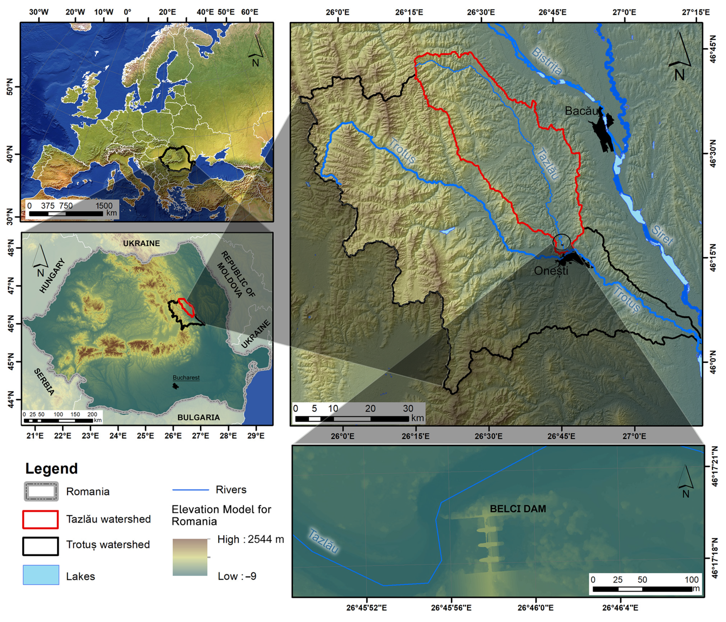
The study area, namely that of the dam of the former Belci lake, is located within the Tazlău river basin, near the confluence of the latter with the Trotuș River, in Romania (Figure 1). The surface of the drainage basin has been calculated at 1101 km2, while the watershed has a length of 188 km. A third of the basin covers a mountainous area (north-west), while the other two thirds expand across hills and valleys (centre and south-east). Belci lake itself had a surface of approximately 250 ha, a length of 3.7 km, and could retain a volume of 12.5 million m3 of water.
On the night between 28–29 July 1991, following a period characterised by a synoptic context marked by torrential rainfall—favouring the oversaturation of the pedological layer of the entire Carpathian area—the most severe hydrotechnical accident in Romania’s recent history took place, leading to the destruction of Belci dam and reservoir, the loss of 25 lives, and significant material damage. The causes were, as mentioned, an excessive amount of precipitation falling upstream (100–150 mm/90 min), as well as a power shortage at the micro-hydropower system, located downstream (triggered by technical difficulties), which made it impossible to operate the mechanical equipment that could have opened the floodgates of the dam. Following this intense rainfall, the flow rate of the Tazlău river increased suddenly, from 6 m3/s to 1800 m3/s. The rupture of the dam caused a 9 m-high wave, which flooded Slobozia village, located in its close proximity. Given that the large quantity of water that entered the lake could not be channelled efficiently downstream, through the flood gates, the water level exceeded the height of the left-side earthfill dike, digging a funnel-shaped breach in the dam. This overtopping failure allowed the entire water in the lake to be emptied.
In order to obtain a clearer, more quantitative perspective of this accident, modern morphometric analyses, based on the use of a drone, structure from motion (SFM) techniques, as well as measurements and corrections carried out following telemetric principles, were undergone. The aim was to devise an efficient and relatively inexpensive (compared with the commercial alternatives) methodological workflow to generate the digital terrain model (DTM) derived from the digital surface model (DSM), with elevation-related corrections. The main means of acquiring data were, therefore, a DJI Phantom 2 v2.0 drone, fitted with a GoPro Hero4 camera. Data processing was performed using specialized software, Agisoft PhotoScan Professional, Educational License [14]. Previous analyses have shown the utility of generating a numerical model for terrain hypsometry, and the results obtained are similar to those generated by means of a Leica Geosystems ScanStation [15]. Alongside classical satellite-based remote sensing studies regarding vegetation-related aspects [16] or agricultural approaches [17], modern techniques have begun to encompass the use of UAVs more frequently in geo-spatial analyses. Previous studies have proven the use and high accuracy of UAVs, especially for small areas, applied in different fields of analysis: floods [18,19,20,21,22,23,24]; geomorphology [25,26,27,28,29,30,31]; ecology [32,33,34,35,36,37,38]; archaeology and architecture [18,39,40,41,42,43,44,45]; or glaciology [46,47,48,49]. UAVs are currently being used with increasing frequency in ecological studies, such as those seeking to determine the above-ground biomass from canopy volume or the carbon content of dryland and semi-arid ecosystems, using structure from motion (SFM) photogrammetry [50]. Romanian literature has focused mostly on the methodological aspects of UAV applications [51,52].
The main objective of the present analysis is to generate the DTM for the study area, before and after the rupture of the dam. Therefore, the surface of the breach section, through which the entire water of Belci lake was spilled during the flood of 1991, and the volume of dam material removed, were also calculated.
2. Materials and Methods
International sources on UAV-based methodology [53,54,55,56,57,58,59] are of both older and more recent date and, therefore, their findings can be subject to potential modifications and updates. The broad applications have introduced multiple types of approaches in morphometric measurements using UAVs. All of these studies are thoroughly quantitative in approach and express the high importance that UAVs have from different perspectives. Some studies address the accuracy of drone-originated, image-based geo-spatial layers [53,54], or the detection of small objects [57] while others tackle the issue of automating as much of this process, as possible [56]. Different types of sensors (RGB or Lidar, for example) can provide airborne data for different applications, such as agriculture [48], geomorphological processes [58], or even flood analysis [59]. Therefore, the recent diversification in drone-related studies, as well as their high accuracy results, has consolidated their diverse role in scientific studies in numerous geo-spatial domains.
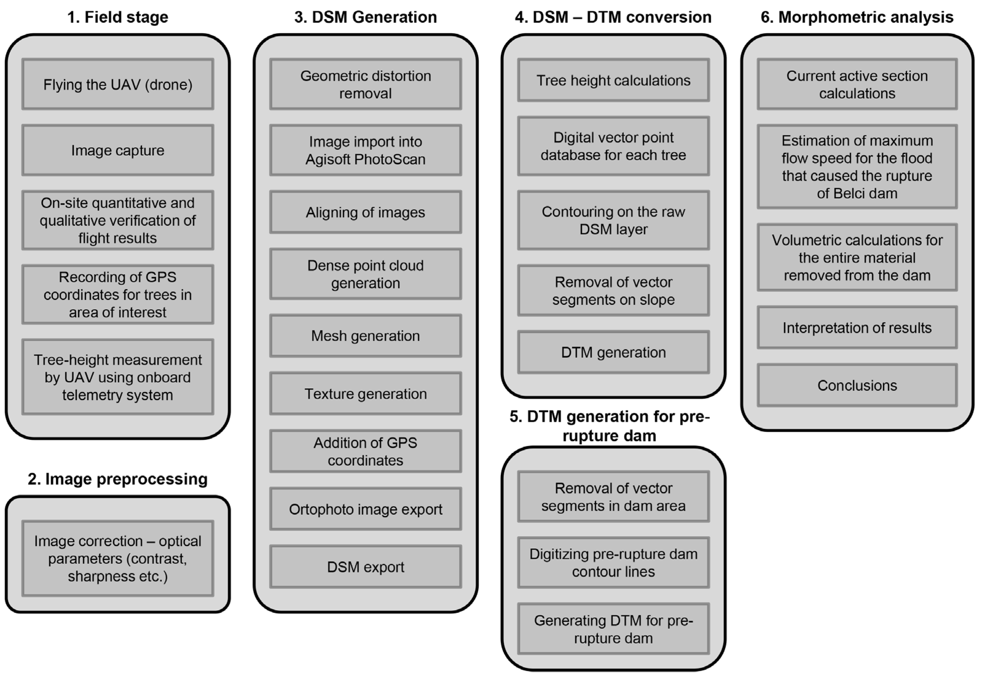
The present study involved several steps, from the field stage to the interpretation of the final cartographic materials generated. It started from the acquisition of aerial imagery, by means of a Phantom 2 drone, to examine the dam itself and to determine the height of certain trees from the left-side hilltop in the study area, which were then removed from the DSM. What followed was the pre-processing stage of these images, which involved making geometric corrections in order to facilitate their interpretation by the Agisoft software (version 1.4.0); to aid in generating a DSM layer, useful in the identification of the geometric elements present in each image; and to ensure a better connection between images and common items. The third stage involved semi-automatic processing by means of Agisoft PhotoScan Professional, during which the images were converted into a DSM and digital orthophoto layer with geographic coordinates. In recent literature, the DSM generated for a predominantly woody area is frequently described as a canopy height model (CHM), with the latter being of interest mainly in ecological and biometric studies [60,61,62,63,64]. Given that the methodology employed in converting the raw data into cartographic materials is based on regular, visible-spectrum images (and not LIDAR-type points, which would have generated pre-classified layers, eliminating the need for further corrections), a correction stage was applied to the DSM, in order to remove the arborescent vegetation located on the slope located to the left of the dam breach, which would have generated errors in calculating the area of the breach section and the volume of material removed, as a result of the 1991 flood. Following this, the DTM of the entire dam was also generated in order to highlight the difference between its current state and the dam state prior to the rupture (and to identify the values mentioned above). Once the cartographic materials were complete, the calculations were made, and the results were interpreted. Although these steps are, indeed, time-consuming and the methodology may seem fairly complicated, each stage contributes to the minimization of the number of potential errors (Figure 2).
The first stage in generating the numerical terrain models and the cartographic materials derived from them, deals with the acquisition of the aerial imagery upon which structure from motion (SFM) techniques are based. This involves a previous survey of the study area in order to identify potential obstacles that may hinder the flight of the drone, such as:
- high-voltage cables, which may confuse and induce calibration issues into the crucial spatial orientation mechanisms of the device;
- difficult-to-access areas, which require a flight path wide enough to acquire images of entire objects and landforms.
The potential of drones to be used in remote areas is one of their great advantages [65]. The manner in which a drone is operated must, nevertheless, ensure a maximum distance that guarantees constant control, but is still short enough to allow the transmission of live telemetry and video feed.
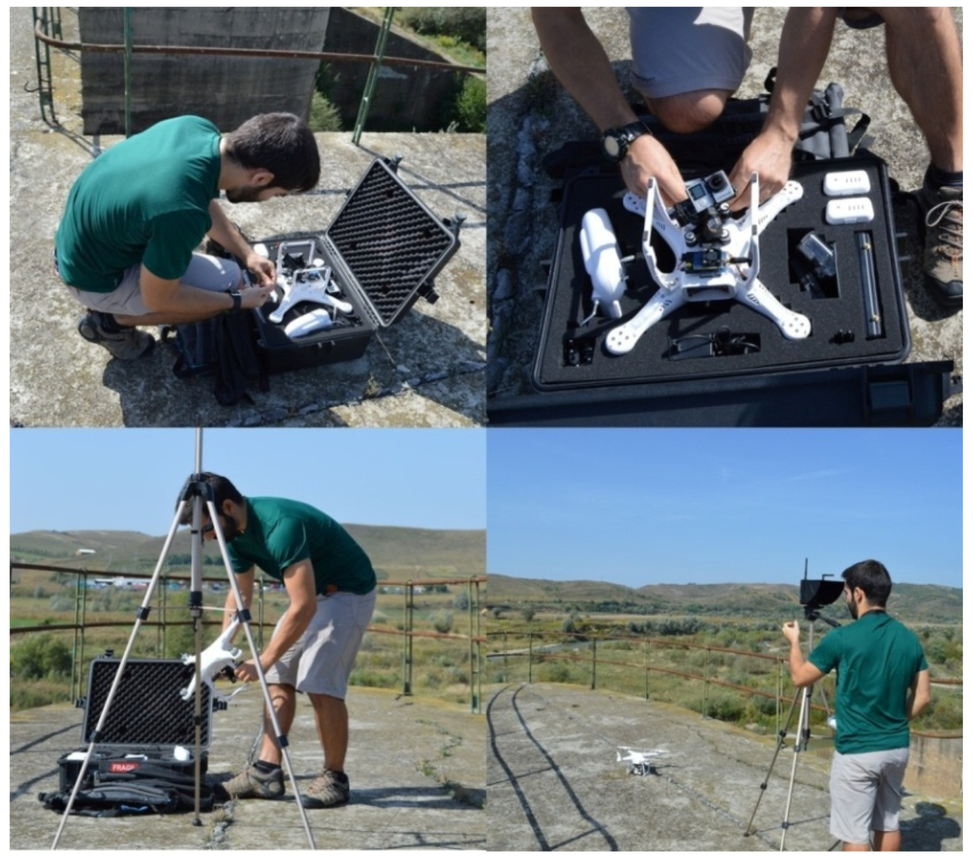
A series of procedures, carried out in a pre-established order, were necessary for the preparation of the flight so as to ensure the proper collection of aerial images. Weather conditions (visibility, wind, humidity, temperature) had to be adequate. The perimeter required for launch must be open, obstacle-free and high enough to guarantee a permanent signal to maintain remote control over the drone. After the necessary equipment is mounted, the camera is attached to the gimbal and adjusted, this is followed by the antenna of the FPV system, the propellers and then the drone battery. The ground station is composed of a double-channel FPV station and a remote control (Figure 3).
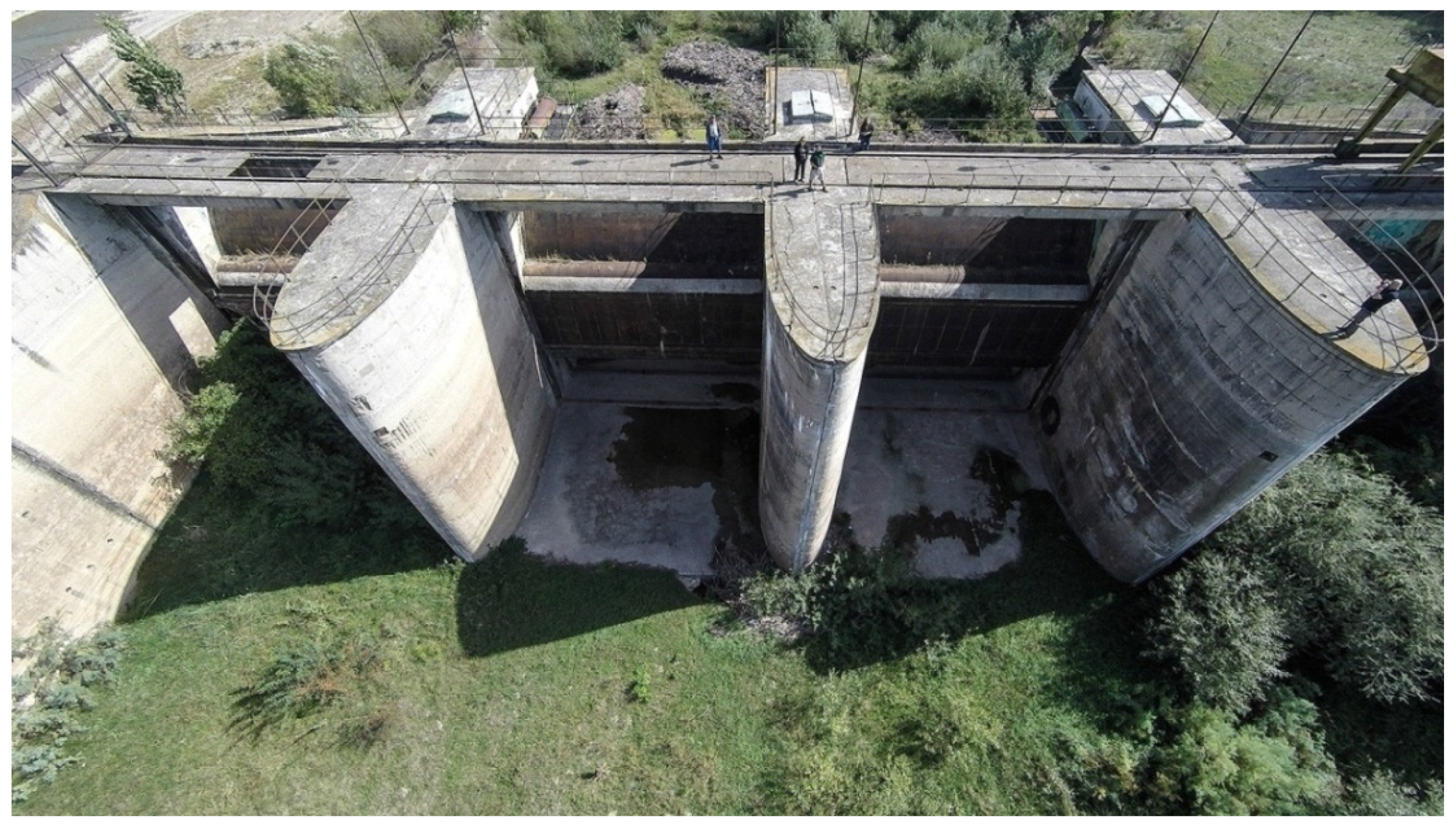
The flight path was planned out in a scanning-type mission that allowed the capturing of a sufficient number of overlapping images of the study area, taken from adequate angles [66]. The aim was to obtain sufficient aerial images with the device oriented vertically, toward the Nadir point, as well as photographs taken from more acute angles—45° against the topographic surface plane. Therefore, images were obtained for all instances in which objects or landforms could have been covered by shadows or where many of their details would have been obscured. Moreover, sufficient images were collected in order to avoid the omission of important frames with facets of the items of interest (such as the individual flood gates). One of the challenges encountered during the present study was related to the dam itself, as capturing the details between the flood gates, including the towers and the side walls required numerous aerial images, out of which 152 files were selected for final analysis (Figure 4).
Once the flight was complete, the aerial images were verified in order to ensure that they are of sufficient quantity and quality, since a potential error or technical difficulty could have compromised the results. Image calibration was carried out using Agisoft Lens [14] and any geometric distortions caused by the camera lens were mitigated and accounted for. This particular piece of software is able to calculate calibration parameters (f, xp, yp, k1, k2, k3, p1, p2) by means of a test screen, and to generate precise values for any type of camera used. For studies conducted on smaller areas, cameras such as the GoPro Hero 4 Black, used in the present case, can be used successfully, because, though the geometric distortions are significant, the final errors are low (0.2–1.5 cm) and of negligible value, especially at the scale of the current study [67,68].
Open-source alternatives, such as VisualSfM + CMPMVS [69,70,71,72] are available, but they display significant limitations regarding the degree of control over their functions, in particular in terms of the possibility of adding geographic coordinates in late stages of the processing workflow. As a result, Agisoft PhotoScan Professional, which offers high-accuracy results (centimetre-level precision, or even sub-centimetre) when provided with high-quality images [73,74,75,76], was considered the better alternative for the current study. Its applicability has been proven during several other morphometric studies, carried out in fields such as geomorphology [28,73,77], glacier analysis [78], flood analysis [19], etc. Even studies based on aerial images obtained using kites [79,80], or on underwater images of coral [81], have highlighted the utility and increased precision of results generated using the Agisoft package.
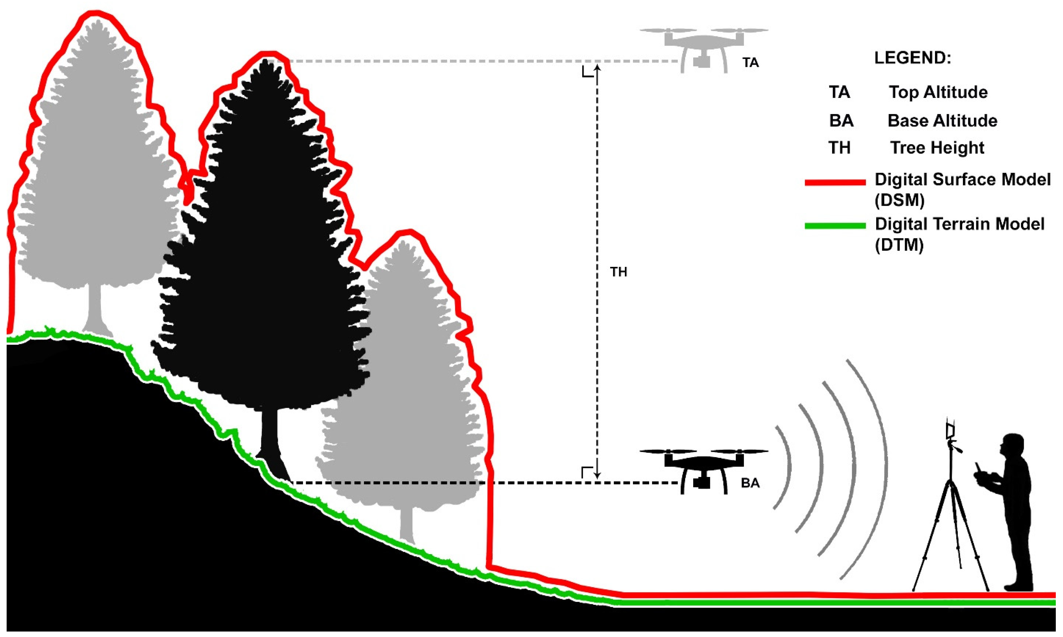
The primary image processing stage, by means of Agisoft PhotoScan Professional, led to a DSM in need of morphometric corrections, given that the vegetation (trees or shrubs) do not correspond to the topographic surface. For the correction of the numerical model, the drone was used once again. There have been previous studies involving tree height according to SFM principles, but also based on LIDAR data [60,82,83,84,85]. In our current study, issues were encountered only on the northern slope of the section of Belci dam earthfill dike, which has remained open. The trees on this slope were first numbered, then the geographic coordinates of each one were registered with the help of a GPS device. Afterwards, flights were carried out, during which the telemetry system, which records the relative drone altitude in real time on the ground monitor through a first-person view (FPV) was employed. The drone (DJI Phantom 2 v2.0) includes a gimbal (DJI Zenmuse H4-3D) which stabilizes the camera, including under windy conditions., with an error of +/−0.02° (for pitch/roll movements), and +/−0.03° (for yaw) [14]. Even on a windy day, the measurement error will not exceed 0.5 cm if the drone is piloted to a location 10 m away from the subject that it is capturing images of, with the GPS mode activated, for stationary flight. Therefore, if the camera is positioned perfectly horizontally on the gimbal, the relative altitude of objects in the exact centre of the FPV screen is the same as that of the drone at that specific moment (Figure 5).
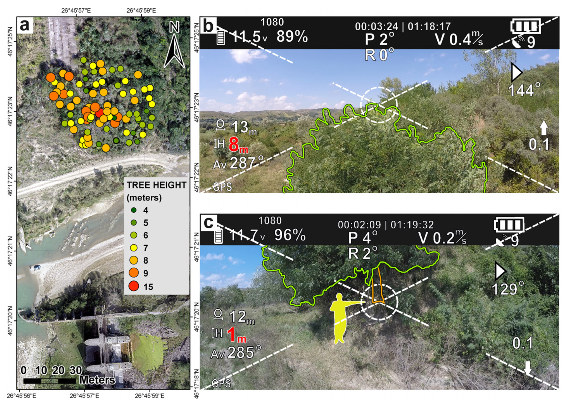
The principles according to which this type of measurements functions are as follows: the drone operator initiates the flight at the base of the tree, in order to record the relative altitude of its base at topographic level, which is then transmitted via the drone’s telemetry system to the operator. Then, the device is flown to the altitude of the top of the tree, recording the new value. By calculating the difference between these two values, the height of the tree is established. These steps were repeated for each tree (the numbers shown in red, in Figure 6). One drawback to be noted is the fact that, where the drone could not fly as a result of dense vegetation, it was carried by hand to the roots, with its engines turned off (to avoid potential accidents), the relative altimetry value was recorded, after which the drone was launched, in order to record the altitude at the top of that particular tree. This was possible due to the precise gimbal functionality, low build/tolerance errors, and close proximity to the trees.
Starting from these values, a database with the heights of the trees that were required to be removed from the DSM could be compiled. Using the GPS coordinates previously recorded, a shapefile with the altitudinal values for each tree was created. The altitude values corresponding to the points on the shapefile were verified on the DSM, and the values on the raster were transferred to the attribute table. The difference between the altitude on the DSM and the height of the trees was calculated. The newly obtained values represent altitudinal points of the actual topographic surface. The contouring function was then applied to the DSM, the area covered by vegetation was delineated, and the contour curves of the problematic area were eliminated. The digital elevation model is re-generated based on the curves and the newly created points, leading to a corrected DTM. This approach was dictated by the fact that the use of an altimeter, however advanced, to directly record points under the foliage would have led to inadmissible errors (up to 15–20 m on the Z axis).
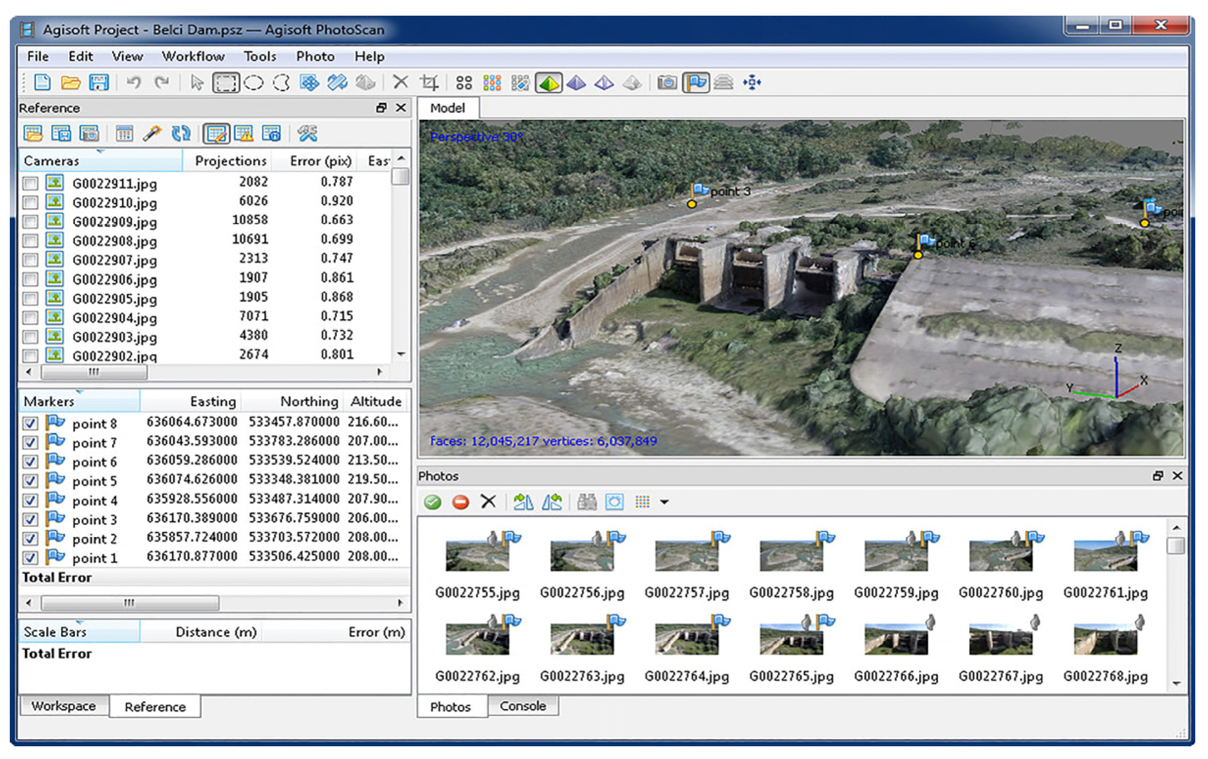
The stage involving Agisoft PhotoScan Professional required initial importing and generating of specific intermediary layers before the finite cartographic products could be exported (Figure 7). The frames were aligned and a dense tridimensional point cloud was generated, followed by a mesh and a texture. The georeference points were then added, and the model was exported both as an orthophoto and a digital surface model (DSM). Given that the images were in the visible spectrum, these georeference points were easily attributed inside Agisoft software, more so than by using the alternatives [86]. The final steps involved the following: calculating the active section based on a transect along the length of the dam; calculating the volume of material removed by the flood through an algebraic subtracting operation based on pre-rupture and post-rupture rasters of the dam; and estimating the speeds of the water evacuated from the lake through the active section. The pre-rupture layer was generated by interpolating contour lines derived from the original layout of the dam, before the breach occurred. In order to maximize compatibility and accuracy, and mitigate volumetric errors during final calculations, this raster was created in accordance with the same projection and spatial resolution of the layer of the post-rupture state, generated through structure from motion techniques.
3. Results
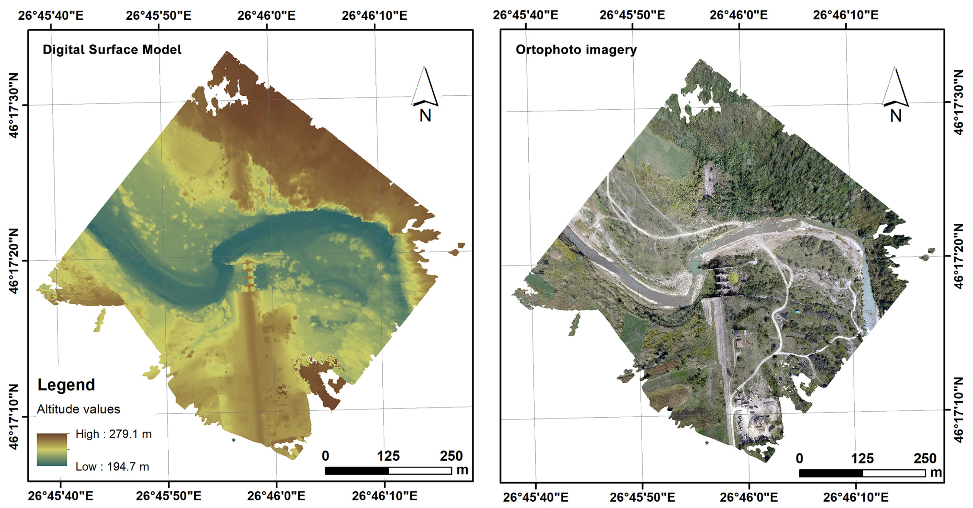
The application of the methodology described above led to the generation of the following primary cartographic materials for morphometric analysis: the digital surface model and the corresponding orthophoto (Figure 8). The resolution at which both thematic layers were generated, for a single pixel, was 7 cm × 7 cm (according to the Agisoft report: 0.0704 m/pix, and a point density of 201.329 points/m2). This resolution is high enough to allow for a detailed analysis with negligible measurement errors.
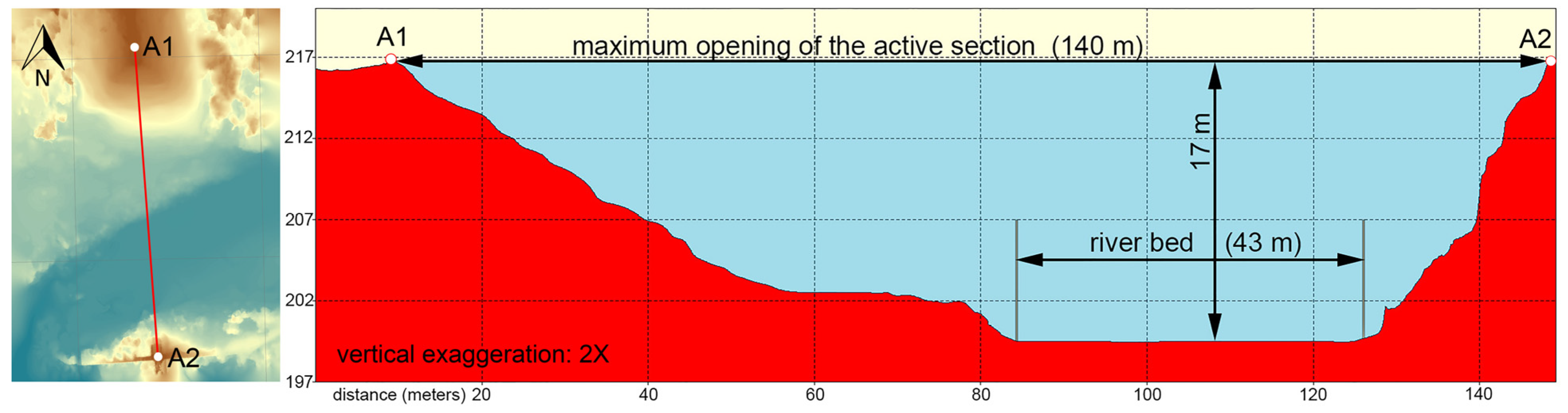
The dam breach active section area was calculated along the dam rupture up to the maximum height of the earthfill dike, more precisely between the 217 m altitude points (which were named in Figure 9: A1 and A2), located at the top of the northern edge of the concrete dam, and the highest current altitude of the left dike, which was overflown in 1991, causing the rupture of the dam. From a vertical perspective, the active section is regarded as stretching between the base of the current minor riverbed and the highest point of the former dike (217 m altitude).
After the cross-section profile was generated, the surface of the active section was calculated by means of image-editing software. The simplified steps involved were the following: the number of pixels located inside the active section was identified, the surface of each one was calculated, and the two values were then multiplied in order to precisely obtain the surface of the active section, expressed in m2.
For expressivity reasons, the active section is represented with a twofold vertical exaggeration. Obtaining the surface of a single pixel required the calculation of both length and width of a particular pixel, because, though the pixel is square, the metric values represented are different for each side. The horizontal side was calculated based on 241 pixels, corresponding to a real distance of 20 m. A simple division led to the determination of the length of the horizontal side of a pixel as 8.29875518 cm (0.0829875518 m). The same steps were taken for the vertical side, and a length of 5 m was calculated, corresponding to 118 pixels. Therefore, the vertical side of a pixel is 4.2372881355 cm (0.042372881355 m).
The real surface of a pixel, calculated by multiplying the values above, is 0.00351642168 m2. Through automatic selection, a total number of 121,698 pixels could be identified within the active section. Once the overall surface, expressed in number of pixels, and the surface of a single pixel were known, the real surface of the active section, 427.94 m2, was calculated. Other morphometric properties of the section were also calculated, such as its current maximum opening (140 m) and height, or the width of the current riverbed (Figure 9).
Once the surface of the active section had been calculated, the simple introduction into the equation of a flow value could lead to the estimation of the maximum speed with which the water was evacuated from Belci lake during the 1991 flood. There are, in fact, two flow values: 1550 m3/s—the flow rate recorded at the Helegiu station—and 2100 m3/s—the reconstituted flow rate at the dam at the moment of the rupture (these values were calculated by the Water Basin Administration). This latter value, and a surface of the active section of 428 m2, were taken into account in order to estimate water velocity. The issue was, however, that water has the greatest energy at the beginning of a flood, when the lake has a maximum retention level, and the active section is yet to develop its current opening. As a result, different evacuation speeds were calculated for different values of the active section, every 50 m2 (Table 1).
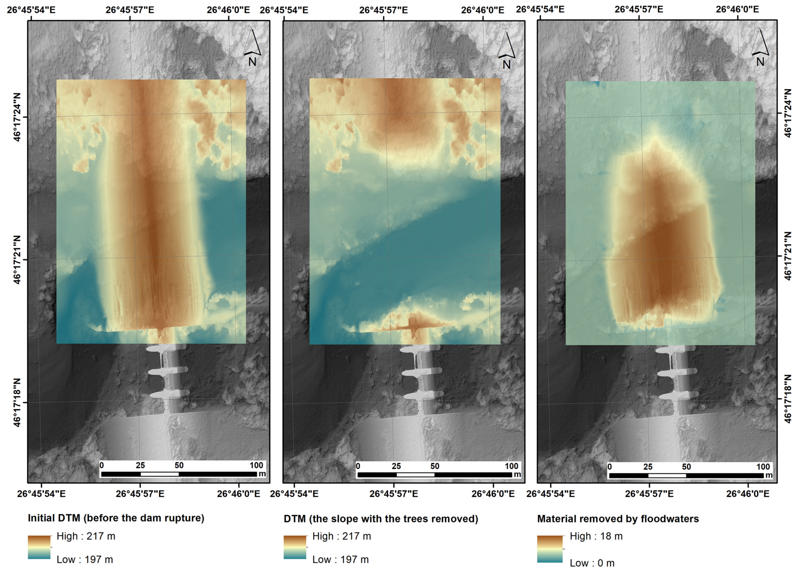
These values range between 17.6 km/h and 75.6 km/h, with the highest of those being registered at the beginning of the flood, when the surface of the active section was reduced and the lake was still completely full. Towards the end of the flood, the speed decreased, along with water volume in the lake, while the surface of the active section increased, up to its maximum size, as a result of the erosive action of the water. The creation of this active section on the night that the Belci dam was breached involved the removal of a very large volume of material from the left dike. This volume of eroded material was calculated using the two digital elevation models, namely that of the area prior to the rupture of the earthfill dike, and that which reflects the current state. The raster calculator function of ArcGIS was applied to the raster layers of the two models in order to identify the volumetric difference between them. The raster of this difference represents a digital model of the eroded earth volume, indicating the location from which the material from the dike was removed.
Starting from this spatial layer, two methods were employed in order to accurately calculate the volume of material removed by the flood. The first method (the manual method) started from the premise that the difference between the two raster layers generated a layer containing nothing more and nothing less than the material eroded as a result of the flood. The surface of a single pixel could easily be calculated. A multiplication between the surface provided by the number of pixels (and their corresponding surface) and the mean value of the former, from the surface of the entire raster file, led to the desired volume value. The numerical model corresponding to the volume of eroded material includes 4,253,568 pixels. The surface of a pixel is 0.0049656 m2, hence the total surface is 21,122 m2 (this is not the surface from which material was removed from the dike, but the entire surface, which includes the difference up to the rectangular spatial extension of this numerical model). The mean pixel value is 3.46575080633 m (in height). The process of multiplying the surface and the mean pixel value reveals a volume of 73,203.3 m3 (the approximate equivalent of 20 Olympic-sized swimming pools).
For validation purposes, a second, automatic method was used, namely the surface volume function of ArcGIS. Starting from a numerical terrain model, this function allows the calculation of a volume with certain parameters (higher or lower than a certain altitude or using another thematic layer as reference plane). Running this function led to the identification of a total area of 1.4 ha, over which the entire material was removed from the dike. The volume calculated automatically by this function was 74,281 m3, a very similar value to that calculated manually. The 1.45% error is within negligible limits. Therefore, starting from the two main layers (the elevation model prior to the dam rupture, and the one after the event), a third layer could be generated (Figure 10), and the volume of material removed from the dike was calculated with high accuracy.
4. Discussion
The field of water environment is very broad and addresses numerous methodologies and types of studies. These can range from wetlands, or water resources, all the way to flood risk, runoff, or erosion. These types of analyses can be performed more efficiently and from multiple perspectives when using a drone. Firstly, this involves temporal advantages, due to the quick deployment times and image acquisition times when using drones. This facilitates the field work stage, which can be done faster and more efficiently. Secondly, drones can fly over hard to reach places that would otherwise be inaccessible to humans. Thirdly, there are cases of areas which are dangerous from a physical, chemical or generally from an environmental perspective. In these areas, the drone can operate normally, while also acquiring data and keeping the operator safe and far from potential risk. Another important aspect is the non-invasive character of using a drone, which has a very small impact on the environment (direct human access is not necessary, e.g., via a boat; physical interactions with local species are minimized; the ecological stress can be significantly lower, especially when using more silent and longer-ranging drones; etc.). Lastly, the cost of operating a drone is usually significantly lower than multiple days field campaigns for measurements, as these include multiple participants; resources; logistics; more expensive gear, such as survey equipment; etc. All of these arguments emphasize the role that UAVs have in the present analyses, as they are a key tool in modern water environmental studies. Therefore, photogrammetric analyses, by means of drones and through structure from motion techniques, have a broad appeal in environmental water studies.
In addition, compared with traditional methods for generating terrain models, such as using a total station (or a theodolite), a prism pole, or a high accuracy survey-grade GPS receiver, the drone has several advantages and disadvantages. The total station method requires a multiple person team, which would operate each piece of equipment individually and require more manpower to transport the equipment. On the other hand, the drone can be transported, set up, and operated by a single operator, reducing the number of people that need to be present at a job site, and thus the cost of human resources. Another aspect needed to be taken into consideration when using a drone, is the deployment time, which is shorter in case of commercial drones, than when using a total station-based solution, which frequently takes a long time to acquire a stable GPS signal in order to achieve higher accuracy. The drone commonly acquires satellite signal in a matter of a few seconds—2–3 min—and can then be flown. However, when using a drone, and when requiring maximum spatial accuracy, ground targets need to be used (also known as ground control points—GCPs). These must be spread out manually and fixed on the ground across the entire study area, and their individual location should also be registered via a high-accuracy GPS receiver. This would take a significant amount of time and would increase cost, meaning that they would no longer be efficient in terms of time or cost. However, this extra step when flying a drone would ensure the cm-level accuracy of the results, provided that the GPS receiver used to register the GPS’s position had that kind of survey-grade accuracy.
Another benefit when flying a drone is the reduction of the potential for human error, which is significantly lower during autonomous flight missions, compared with manual field measurements using a total station, or in a situation in which the operators are either tired or not sufficiently experienced. Total station measurements can have multiple points of entry for potential errors, such as incorrect projection/datum selection, total station levelling, choosing appropriate/representative points for measuring with the prism pole, inputting incorrect values corresponding to pole height, etc. In addition, the total station operator generally needs to be more knowledgeable and skilled than a drone operator when conducting field surveys.
On-field validation is another issue with newly recorded total station datasets: while the drone images can be downloaded and swiftly imported into an SFM software, such as Agisoft Metashape, and then aligned to verify the complete and direct coverage during the field stage, the total station datasets generally require more time to be precisely analysed upon their return to the office.
The details in the final products are usually higher when using a drone solution, considering that the drone interpolates points for the entire study area, while the total station solution only filters several interest areas. Drone-generated results have a spatial data density of hundreds or thousands of points per square meter, while the total station has to generalize, and will not have the same data density, as drone-generated layers.
The drone will always be a better solution when conducting surveys in areas impossible to be physically reached by human operators, therefore increasing the amount of detail in certain survey missions.
Furthermore, from a technical perspective, drones generate images which are processed into 3D models, and which retain their colour in the final orthophoto image, therefore providing an extra layer of information that is not recording during total station surveys. In addition, there is the need to emphasize the spatial dynamics advantage of the drone, due to the fact that flight missions can be stored and used in future surveys over the same area, with ease. Therefore, the repetitive character of drone surveys is a definite advantage over the total station solution.
As previously mentioned, the time required to perform a drone survey is significantly lower than a complete total station survey, being potentially limited to only 1–2 h of effective field work (and even under 1 h, for small area flights).
Arguably, the most important aspect when comparing these solutions is the overall cost they require for equipment, operators and staff, software, and other costs. In the case of the drone, a low-cost solution can be estimated at 2000–3000 dollars/euros, while a complete total station solution will be tens of thousands of dollars/euros. Furthermore, the cost of hiring skilled staff, and multiple vehicles dispatched in the field is added on top of the equipment.
However, compared with more modern techniques, such as ground-based laser scanning, the drone loses the time and accuracy advantage, but at a high equipment cost.
All of the arguments mentioned above emphasize the advantages and real-world decisions taken in favour of using drones when conducting studies, such as the current study, that are related to volume measurements for hydrological risk events.
The current results reveal a total earth volume, removed from Belci dam, of approximately 73,000–74,000 m3. However, this value is subjected to a few processes and the lack of previous temporal measurements, which could possibly induce errors. Fluvial geomorphology implies that the variance in flow rates and water levels will induce lateral erosion, attrition, etc. over time. Rivers are subjected to permanent hydraulic dynamic processes, which can take place over the span of decades, or just minutes. Unfortunately, since the Belci dam break accident, thorough measurements of the breach have not been performed, and its state has been kept the same, without any intervention, so there are no quantitative numbers that could be used to extract the riverbank erosion, or talweg migration etc. However, through empirical methods, and by asking local people, it can be stated that the volume of earth eroded after the dam break is negligible, considering that there were no similarly significant floods following this dam break event, and that the river has not been seen/measured to exit its current banks. Furthermore, the core of the dam is made of clay, and is therefore impermeable, so that no more water has managed to infiltrate in such high volumes as to make the remaining ruins of the dam collapse even more. However, this uncertainty in the volumetric/morphological measurements, over the span of over 30 years, makes it impossible to completely and accurately evaluate the exact volume of earth eroded by the event itself. This is a limitation of the model, but it is considered to be negligible, considering that it is extremely difficult to accurately measure the exact amount of earth displaced by a dam break accident, even when measuring the site a few days after the event. This is due to the fact that most dams that fail have existed for multiple years, that the silting process has been active (considering that large lakes generally have large hydrographic basins), and also that the water infiltration into the ground is very high. For this reason, the earth erosion process itself does not stop at the exact ending time of the flood hydrograph, but rather takes weeks/months to stabilize. This due to the soft nature of sediments, which cannot be thoroughly distinguished from clay or other similar types of dam building material through topographic measurements. This implies there will always be an error in measuring displaced volumes of earth from dam breaks, even under optimal conditions for such measurements, immediately after such events. This limitation of the study (of possibly overestimating the total removed earth volume) is accepted due to the physical constraints of measuring the break by any other means, and also due to the lack of other previous measurements.
Another limitation relates to the fact that the drone was used as a relative altimeter to measure the height of the trees, which was difficult at times in which the general vegetation cover was dense. Therefore, some tree measurements required more attention and time, because the spotter (the person aiding in the indication of the base of the tree to the drone) had occasional difficulties in reaching some trees. However, though the drone altimeter is accurate to units of only 1 m, the differences between values were verified by measuring a building with an exact known height and is therefore considered accurate. This study did not require the need for absolute hypsometric values in order to measure tree heights, but rather accurate relative altitude, so that the simple mathematical subtraction between top and bottom altitude values would indicate the height of the tree. However, a limitation regarding this approach can be derived from the fact that certain branches are not interpolated accurately from SFM techniques, therefore the overall value of the tree height could be slightly altered for trees with thinner top branches. Despite this, these values would not extrapolate to an added error of more than 1 unit of measurement of relative height from the drone altimeter (therefore, 1 m).
Furthermore, there are a few technical limitations that are noteworthy. Probably one of the biggest technical limitations of this type of drone (also known as a “quad copter”) is the flight time. Commonly, flight times are 15–20 min of real mission flight, however, newer drones can fly up to 30–40 min. This could be a concern due to the time required to charge batteries between flights, or the need to purchase multiple sets of batteries. This could be both a financial and a temporal constraint, provided that some areas would require more time to be properly covered with sufficient aerial images. In relation to this limitation is another, regarding the desired, final spatial resolution. If such studies require a higher spatial resolution than 5–10 cm (also known as ground sampling distance—GSD), some flight parameters need to be adjusted, in order to provide this increased accuracy. Firstly, the relative flight altitude of the drone needs to be lower, in order for the camera to capture more detail. This implies that, at the same side overlap of 70–80% (required for quality results), the drone has to fly through more sections in order to cover the same study area, therefore increasing the flight time and number of batteries used.
Considering the fact that the study area is relatively reduced in size, the use of this type of drone (quad copter) is appropriate because of its abilities to cover the entirety of the area. However, this type of drone is only feasibly useful for small study areas with specifically localized phenomena and which span over a maximum surface of a few tens of hectares. When study areas are larger than this, quad copter drones are highly inefficient, therefore usually requiring the use of wing-type drones.
Another potential limitation could be the image resolution (expressed in megapixels), which is not necessarily relevant for artistic photography, but significantly relevant for details when flying photogrammetric missions. This is highly dependent on the camera model used, but common low-cost drones have standard resolutions of approximately 20–48 megapixels, therefore the final product is not altered in terms of detail, or spatial resolution. This limitation would only apply when studying very high detail phenomena, such as surface erosion, or soil micromorphology.
Finally, some relevant limitations are related to using electronic flying equipment in the proximity of high voltage wires, or other sources of interference (especially in the 2.4 GHz or 5 GHz frequency ranges, where there are numerous devices in use, all over the globe). This would imply recalculating the flight routes/mission altitudes etc.
Alongside the entire volume of water that was evacuated from Belci lake, through the dam breach, it is also important to take the sediment transported downstream from silt and dam material into account. This is due to the fertilizing nature that such sediments frequently have on the floodplains used for agricultural land, located downstream, which future crops could have eventually benefited from (although this has not been studied in particular).
Today, the dam is still non-operational—there have been several proposals to rehabilitate it over the previous years, however reconstruction measures have yet to be taken. At the time of writing this paper, the Siret Water Basin Administration is finalizing the necessary documentation necessary to rehabilitate the dam, with national and international funding. However, these are very early stages in the project, and actual physical interventions on the dam have yet to be performed. Despite there being several attempts to rebuild the dam over the previous years, due to a lack of funding this has yet to be undertaken.
5. Conclusions
The study of the hydrotechnical accident of July 1991 is of great importance in hydrological research, and the application of modern techniques greatly facilitates it, improving the accuracy of the results and reducing the amount of time dedicated to processing. The drone has proven to be a useful, low-cost tool in hydro-geomorphometric research, by capturing aerial imagery with the purpose of generating a digital surface model (with the corresponding digital terrain model) and high spatial resolution orthophoto imagery. Its main drawback, however, is the requirement to remove elements that are not part of the numerical terrain model; in other words, the need to correct the DSM in order to convert it into a DTM.
The generation of the numerical terrain model has led to the following derived layers: a raster layer consisting of the total volume of eroded material as a result of the flood that ruptured the left dike; the active section, necessary for identifying the span of the area through which the water in Belci lake was evacuated; and further calculations, related to the estimation of water speeds. The total eroded volume was calculated at approximately 73,000–74,000 m3.
Another novelty consists in the methodological approach used to determine the height of each tree, in order to create a vector point layer with all the trees that were eliminated from the DSM. This step was undertaken to generate a vegetation-free DEM of the breach area. This was performed using the regular lens of the drone, in the optical spectrum, by calculating the difference between the relative altitude of the drone position, between the base and the top of each tree.
The application of the intended drone-based methodology during the current study has proven flexible, fast, precise, non-intrusive and with a reduced execution cost, and it has led to relevant results, from a morphometric perspective.
Author Contributions
Conceptualization, A.E.; methodology, A.E. and C.C.S.; software, C.C.S. and M.I.; validation, A.E., C.C.S. and M.I.; formal analysis, A.E.; investigation, A.E. and M.I.; resources, C.C.S.; data curation, A.E. and C.C.S.; writing—original draft preparation, M.I. and A.E.; writing—review and editing, A.E., M.I. and C.C.S.; visualization, M.I. and C.C.S.; supervision, A.E.; project administration, A.E.; funding acquisition, A.E. All authors discussed the results and contributed to the final manuscript. All the authors of this study contributed equally to the current article. All authors have read and agreed to the published version of the manuscript.
Funding
This research was funded by a grant of the “Alexandru Ioan Cuza” University of Iasi, within the Research Grants program, Grant UAIC, code GI-UAIC-2021-02.
Data Availability Statement
Data sharing not applicable.
Acknowledgments
This work was supported by a grant of the “Alexandru Ioan Cuza” University of Iasi, within the Research Grants program, Grant UAIC, code GI-UAIC-2021-02.
Conflicts of Interest
The authors declare no conflict of interest.
References
- Maghrebi, M.; Noori, R.; Mehr, A.D.; Lak, R.; Darougheh, F.; Razmgir, R.; Farnoush, H.; Taherpour, H.; Moghaddam, S.M.R.A.; Araghi, A.; et al. Spatiotemporal changes in Iranian rivers’ discharge. Elem. Sci. Anth. 2023, 11, 00002. [Google Scholar] [CrossRef]
- Mayo, T.L.; Lin, N. Climate change impacts to the coastal flood hazard in the northeastern United States. Weather Clim. Extrem. 2022, 36, 100453. [Google Scholar] [CrossRef]
- Angra, D.; Sapountzaki, K. Climate change affecting forest fire and flood risk—Facts, predictions, and perceptions in central and south Greece. Sustainability 2022, 14, 13395. [Google Scholar] [CrossRef]
- Finn, B.M.; Cobbinah, P.B. African urbanisation at the confluence of informality and climate change. Urban Stud. 2023, 60, 405–424. [Google Scholar] [CrossRef]
- Cojoc, G.M.; Romanescu, G.; Tirnovan, A. Exceptional floods on a developed river: Case study for the Bistrita River from the Eastern Carpathians (Romania). Nat. Hazards 2015, 77, 1421–1451. [Google Scholar] [CrossRef]
- Romanescu, G.; Nistor, I. The effects of the July 2005 catastrophic inundations in the Siret River’s Lower Watershed, Romania. Nat. Hazards 2011, 57, 345–368. [Google Scholar] [CrossRef]
- Romanescu, G.; Stoleriu, C.C. Causes and effects of the catastrophic flooding on the Siret River (Romania) in July–August 2008. Nat. Hazards 2013, 69, 1351–1367. [Google Scholar] [CrossRef]
- Minea, I.; Iosub, M.; Enea, A.; Boicu, D.; Chelariu, O.E. Hydrological Extremes Anomalies and Trends in Lower Danube Basin: Case Study—Romanian Drainage Area Between Siret and Prut Rivers. In The Lower Danube River. Earth and Environmental Sciences Library; Negm, A., Zaharia, L., Ioana-Toroimac, G., Eds.; Springer: Cham, Switzerland, 2021. [Google Scholar] [CrossRef]
- Iosub, M.; Minea, I.; Chelariu, O.E.; Ursu, A. Assessment of flash flood susceptibility potential in Moldavian Plain (Romania). J. Flood Risk Manag. 2020, 13, e12588. [Google Scholar] [CrossRef]
- Jitariu, V.; Dorosencu, A.; Ichim, P.; Ion, C. Severe Drought Monitoring by Remote Sensing Methods and Its Impact on Wetlands Birds Assemblages in Nuntași and Tuzla Lakes (Danube Delta Biosphere Reserve). Land 2022, 11, 672. [Google Scholar] [CrossRef]
- Corduneanu, F.; Vintu, V.; Balan, I.; Crenganis, L.; Bucur, D. Impact of drought on water resources in north-eastern Romania. Case study-Prut River. Environ. Eng. Manag. J. 2016, 15, 1213–1222. [Google Scholar]
- Niacsu, L.; Bucur, D.; Ionita, I.; Codru, I.-C. Soil Conservation Measures on Degraded Land in the Hilly Region of Eastern Romania: A Case Study from Puriceni-Bahnari Catchment. Water 2022, 14, 525. [Google Scholar] [CrossRef]
- Agapie Mereuță, I.; Luca, M.; Gherasim, P.-M.; Dominte Croitoru, V. Design of GNSS networks for monitoring earth dams deformations. J. Appl. Life Sci. Environ. 2021, 54, 354–369. [Google Scholar] [CrossRef]
- Agisoft Metashape. Available online: https://www.agisoft.com/ (accessed on 15 January 2023).
- Westoby, M.J.; Brasington, J.; Glasser, N.F.; Hambrey, M.J.; Reynolds, J.M. “Structure-from-Motion” photogrammetry: A low-cost, effective tool for geoscience applications. Geomorphology 2012, 179, 300–314. [Google Scholar] [CrossRef]
- Ciutea, A.; Jitariu, V. Thermal inversions identification through the analysis of the vegetation inversions occurred in the forest ecosystems from the Eastern Carpathians. Present Environ. Sustain. Dev. 2020, 14, 29–42. [Google Scholar] [CrossRef]
- Niacsu, L.; Sfica, L.; Ursu, A.; Ichim, P.; Bobric, D.E.; Breaban, I.G. Wind erosion on arable lands, associated with extreme blizzard conditions within the hilly area of Eastern Romania. Environ. Res. 2019, 169, 86–101. [Google Scholar] [CrossRef] [PubMed]
- Brumana, R.; Oreni, D.; Van Hecke, L.; Barazzetti, L.; Previtali, M.; Roncoroni, F.; Valente, R. Combined Geometric and Thermal Analysis from UAV Platforms for Archaeological Heritage Documentation. ISPRS Ann. Photogramm. Remote Sens. Spat. Inf. Sci. 2013, II, 49–54. [Google Scholar] [CrossRef]
- Feng, Q.; Liu, J.; Gong, J. Urban Flood Mapping Based on Unmanned Aerial Vehicle Remote Sensing and Random Forest Classifier—A Case of Yuyao, China. Water 2015, 7, 1437–1455. [Google Scholar] [CrossRef]
- Klemas, V.V. Coastal and Environmental Remote Sensing from Unmanned Aerial Vehicles: An Overview. J. Coast. Res. 2015, 315, 1260–1267. [Google Scholar] [CrossRef]
- Lee, I.; Kang, J.; Seo, G. Applicability analysis of ultra-light UAV for flooding site survey in South Korea. Int. Arch. Photogramm. Remote Sens. Spat. Inf. Sci. 2013, 1, 185–189. [Google Scholar] [CrossRef]
- Perks, M.T.; Russell, A.J.; Large, A.R.G. Technical Note: Advances in flash flood monitoring using UAVs. Hydrol. Earth Syst. Sci. Discuss 2016, 20, 4005–4015. [Google Scholar] [CrossRef]
- Şerban, G.; Rus, I.; Vele, D.; Breţcan, P.; Alexe, M.; Petrea, D. Flood-prone area delimitation using UAV technology, in the areas hard-to-reach for classic aircrafts: Case study in the north-east of Apuseni Mountains, Transylvania. Nat. Hazards 2016, 82, 1817–1832. [Google Scholar] [CrossRef]
- Tamminga, A.D.; Eaton, B.C.; Hugenholtz, C.H. UAS-based remote sensing of fluvial change following an extreme flood event. Earth Surf. Process. Landf. 2015, 40, 1464–1476. [Google Scholar] [CrossRef]
- d’Oleire-Oltmanns, S.; Marzolff, I.; Peter, K.; Ries, J. Unmanned Aerial Vehicle (UAV) for Monitoring Soil Erosion in Morocco. Remote Sens. 2012, 4, 3390–3416. [Google Scholar] [CrossRef]
- Gonçalves, J.A.; Henriques, R. UAV photogrammetry for topographic monitoring of coastal areas. ISPRS J. Photogramm. Remote Sens. 2015, 104, 101–111. [Google Scholar] [CrossRef]
- Lim, M.; Dunning, S.A.; Burke, M.; King, H.; King, N. Quantification and implications of change in organic carbon bearing coastal dune cliffs: A multiscale analysis from the Northumberland coast, UK. Remote Sens. Environ. 2015, 163, 1–12. [Google Scholar] [CrossRef]
- Lucieer, A.; Jong, S.M.D.; Turner, D. Mapping landslide displacements using Structure from Motion (SfM) and image correlation of multi-temporal UAV photography. Prog. Phys. Geogr. 2013, 38, 97–116. [Google Scholar] [CrossRef]
- Mancini, F.; Dubbini, M.; Gattelli, M.; Stecchi, F.; Fabbri, S.; Gabbianelli, G. Using Unmanned Aerial Vehicles (UAV) for High-Resolution Reconstruction of Topography: The Structure from Motion Approach on Coastal Environments. Remote Sens. 2013, 5, 6880–6898. [Google Scholar] [CrossRef]
- Tahar, K.N.; Ahmad, A.; Akib, W.A.A.W.M.; Mohd, W.M.N.W. Full Length Research Paper A new approach on production of slope map using autonomous Unmanned aerial vehicle. Int. J. Phys. Sci. 2012, 7, 5678–5686. [Google Scholar] [CrossRef]
- Niculiță, M.; Mărgărint, M.C.; Tarolli, P. Using UAV and LiDAR data for gully geomorphic changes monitoring. In Developments in Earth Surface Processes; Tarolli, P., Mudd, S.M., Eds.; Elsevier: Amsterdam, The Netherlands, 2020; Volume 23, pp. 271–315. [Google Scholar]
- Christensen, B.R. Use of UAV or remotely piloted aircraft and forward-looking infrared in forest, rural and wildland fire management: Evaluation using simple economic analysis. N. Z. J. For. Sci. 2015, 45, 16. [Google Scholar] [CrossRef]
- Proulx, R.; Roca, I.T.; Cuadra, F.S.; Seiferling, I.; Wirth, C. A novel photographic approach for monitoring the structural heterogeneity and diversity of grassland ecosystems. J. Plant Ecol. 2014, 7, 518–525. [Google Scholar] [CrossRef]
- Fráter, T.; Juzsakova, T.; Lauer, J.; Dióssy, L.; Rédey, A. Unmanned Aerial Vehicles in Environmental Monitoring—An Efficient Way for Remote Sensing. J. Environ. Sci. Eng. 2015, A4, 85–91. [Google Scholar] [CrossRef]
- Wallace, L.; Lucieer, A.; Watson, C.; Turner, D. Development of a UAV-LiDAR System with Application to Forest Inventory. Remote Sens. 2012, 4, 1519–1543. [Google Scholar] [CrossRef]
- Zahawi, R.A.; Dandois, J.P.; Holl, K.D.; Nadwodny, D.; Reid, J.L.; Ellis, E.C. Using lightweight unmanned aerial vehicles to monitor tropical forest recovery. Biol. Conserv. 2015, 186, 287–295. [Google Scholar] [CrossRef]
- Mohan, M.; Richardson, G.; Gopan, G.; Aghai, M.M.; Bajaj, S.; Galgamuwa, G.P.; Vastaranta, M.; Arachchige, P.S.P.; Amorós, L.; Corte, A.P.D.; et al. UAV-supported forest regeneration: Current trends, challenges and implications. Remote Sens. 2021, 13, 2596. [Google Scholar] [CrossRef]
- Ecke, S.; Dempewolf, J.; Frey, J.; Schwaller, A.; Endres, E.; Klemmt, H.-J.; Tiede, D.; Seifert, T. UAV-Based Forest Health Monitoring: A Systematic Review. Remote Sens. 2022, 14, 3205. [Google Scholar] [CrossRef]
- Achille, C.; Adami, A.; Chiarini, S.; Cremonesi, S.; Fassi, F.; Fregonese, L.; Taffurelli, L. UAV-Based Photogrammetry and Integrated Technologies for Architectural Applications—Methodological Strategies for the after-Quake Survey of Vertical Structures in Mantua (Italy). Sensors 2015, 15, 15520–15539. [Google Scholar] [CrossRef]
- Nicolas, P.; Florent, H.; Calastrenc, C. Low Altitude Thermal Survey by Means of an Automated Unmanned Aerial Vehicle for the Detection of Archaeological Buried Structures. Archaeol. Prospect. 2013, 20, 303–307. [Google Scholar] [CrossRef]
- Themistocleous, K.; Agapiou, A.; Cuca, B.; Hadjimitsis, D.G. Unmanned Aerial Systems and Spectroscopy for Remote Sensing Applications in Archaeology. ISPRS-Int. Arch. Photogramm. Remote Sens. Spat. Inf. Sci. 2015, XL-7/W3, 1419–1423. [Google Scholar] [CrossRef]
- Themistocleous, K.; Hadjimitsis, D.G.; Georgopoulos, A.; Agapiou, A.; Alexakis, D.D. Development of a Low Altitude Airborne Imaging System for Supporting Remote Sensing and Photogrammetric Applications “The ICAROS Project” Intended for Archaeological Applications in Cyprus. In Progress in Cultural Heritage Preservation; Lecture Notes in Computer Science (Including Subseries Lecture Notes in Artificial Intelligence and Lecture Notes in Bioinformatics); Springer: Berlin/Heidelberg, Germany, 2012; pp. 494–504. [Google Scholar] [CrossRef]
- Fiz, J.I.; Martín, P.M.; Cuesta, R.; Subías, E.; Codina, D.; Cartes, A. Examples and results of aerial photogrammetry in archeology with UAV: Geometric documentation, high resolution multispectral analysis, models and 3D printing. Drones 2022, 6, 59. [Google Scholar] [CrossRef]
- Ulvi, A. Using UAV Photogrammetric Technique for Monitoring, Change Detection, and Analysis of Archeological Excavation Sites. J. Comput. Cult. Herit. (JOCCH) 2022, 15, 1–19. [Google Scholar] [CrossRef]
- Mihu-Pintilie, A.; Brașoveanu, C.; Stoleriu, C.C. Using UAV Survey, High-Density LiDAR Data and Automated Relief Analysis for Habitation Practices Characterization during the Late Bronze Age in NE Romania. Remote Sens. 2022, 14, 2466. [Google Scholar] [CrossRef]
- Bhardwaj, A.; Sam, L.; Martín-Torres, F.J.; Kumar, R. UAVs as remote sensing platform in glaciology: Present applications and future prospects. Remote Sens. Environ. 2016, 175, 196–204. [Google Scholar] [CrossRef]
- Immerzeel, W.W.; Kraaijenbrink, P.D.A.; Shea, J.M.; Shrestha, A.B.; Pellicciotti, F.; Bierkens, M.F.P.; de Jong, S.M. High-resolution monitoring of Himalayan glacier dynamics using unmanned aerial vehicles. Remote Sens. Environ. 2014, 150, 93–103. [Google Scholar] [CrossRef]
- Gaffey, C.; Bhardwaj, A. Applications of unmanned aerial vehicles in cryosphere: Latest advances and prospects. Remote Sens. 2020, 12, 948. [Google Scholar] [CrossRef]
- Chudley, T.R.; Christoffersen, P.; Doyle, S.H.; Abellan, A.; Snooke, N. High-accuracy UAV photogrammetry of ice sheet dynamics with no ground control. Cryosphere 2019, 13, 955–968. [Google Scholar] [CrossRef]
- Cunliffe, A.M.; Brazier, R.E.; Anderson, K. Ultra-fine grain landscape-scale quantification of dryland vegetation structure with drone-acquired structure-from-motion photogrammetry. Remote Sens. Environ. 2016, 183, 129–143. [Google Scholar] [CrossRef]
- Curiac, D.-I.; Volosencu, C. Path Planning Algorithm based on Arnold Cat Map for Surveillance UAVs. Def. Sci. J. 2015, 65, 483. [Google Scholar] [CrossRef]
- Muraru, A. Some Aspects Regarding “Sense and Avoid” Requirements for UAV Integration in the National Air Space. Incas Bull. 2010, 2, 133–141. [Google Scholar] [CrossRef]
- Harwin, S.; Lucieer, A. Assessing the Accuracy of Georeferenced Point Clouds Produced via Multi-View Stereopsis from Unmanned Aerial Vehicle (UAV) Imagery. Remote Sens. 2012, 4, 1573–1599. [Google Scholar] [CrossRef]
- Lisein, J.; Linchant, J.; Lejeune, P. Aerial surveys using an Unmanned Aerial System (UAS): Comparison of different methods for estimating the surface area of sampling strips. Trop. Conserv. Sci. 2013, 6, 506–520. [Google Scholar] [CrossRef]
- Mathews, A.; Jensen, J. Visualizing and Quantifying Vineyard Canopy LAI Using an Unmanned Aerial Vehicle (UAV) Collected High Density Structure from Motion Point Cloud. Remote Sens. 2013, 5, 2164–2183. [Google Scholar] [CrossRef]
- Turner, D.; Lucieer, A.; Watson, C. An Automated Technique for Generating Georectified Mosaics from Ultra-High Resolution Unmanned Aerial Vehicle (UAV) Imagery, Based on Structure from Motion (SfM) Point Clouds. Remote Sens. 2012, 4, 1392–1410. [Google Scholar] [CrossRef]
- Zhan, W.; Sun, C.; Wang, M.; She, J.; Zhang, Y.; Zhang, Z.; Sun, Y. An improved Yolov5 real-time detection method for small objects captured by UAV. Soft Comput. 2022, 26, 361–373. [Google Scholar] [CrossRef]
- Hussain, Y.; Schlögel, R.; Innocenti, A.; Hamza, O.; Iannucci, R.; Martino, S.; Havenith, H.B. Review on the Geophysical and UAV-Based Methods Applied to Landslides. Remote Sens. 2022, 14, 4564. [Google Scholar] [CrossRef]
- Trepekli, K.; Balstrøm, T.; Friborg, T.; Fog, B.; Allotey, A.; Kofie, R.; Møller-Jensen, L. UAV-borne, LiDAR-based elevation modelling: A method for improving local-scale urban flood risk assessment. Nat. Hazards 2022, 113, 423–451. [Google Scholar] [CrossRef]
- Dandois, J.P.; Ellis, E.C. High spatial resolution three-dimensional mapping of vegetation spectral dynamics using computer vision. Remote Sens. Environ. 2013, 136, 259–276. [Google Scholar] [CrossRef]
- Hernández-Clemente, R.; Navarro-Cerrillo, R.; Ramírez, F.; Hornero, A.; Zarco-Tejada, P. A Novel Methodology to Estimate Single-Tree Biophysical Parameters from 3D Digital Imagery Compared to Aerial Laser Scanner Data. Remote Sens. 2014, 6, 11627–11648. [Google Scholar] [CrossRef]
- Ota, T.; Ogawa, M.; Shimizu, K.; Kajisa, T.; Mizoue, N.; Yoshida, S.; Takao, G.; Hirata, Y.; Furuya, N.; Sano, T.; et al. Aboveground Biomass Estimation Using Structure from Motion Approach with Aerial Photographs in a Seasonal Tropical Forest. Forests 2015, 6, 3882–3898. [Google Scholar] [CrossRef]
- Lin, J.; Chen, D.; Wu, W.; Liao, X. Estimating aboveground biomass of urban forest trees with dual-source UAV acquired point clouds. Urban For. Urban Green. 2022, 69, 127521. [Google Scholar] [CrossRef]
- Gülci, S.; Akay, A.E.; Aricak, B.; Sariyildiz, T. Recent Advances in UAV-Based Structure-from-Motion Photogrammetry for Aboveground Biomass and Carbon Storage Estimations in Forestry. In Concepts and Applications of Remote Sensing in Forestry; Suratman, M.N., Ed.; Springer: Singapore, 2023; pp. 395–409. [Google Scholar] [CrossRef]
- Eisenbeiß, H.; Zurich, E.T.H.; Eisenbeiß, H.; Zürich, E.T.H. UAV photogrammetry. Inst. Photogramm. Remote Sens. 2009. [Google Scholar] [CrossRef]
- Micheletti, N.; Chandler, J.H.; Lane, S.N. Structure from Motion (SfM) Photogrammetry. Geomorphol. Tech. 2015, 2, 1–12. [Google Scholar]
- Balletti, C.; Guerra, F.; Tsioukas, V.; Vernier, P. Calibration of Action Cameras for Photogrammetric Purposes. Sensors 2014, 14, 17471–17490. [Google Scholar] [CrossRef] [PubMed]
- Karantzalos, K.; Koutsourakis, P.; Kalisperakis, I.; Grammatikopoulos, L. Model-based building detection from low-cost optical sensors onboard unmanned aerial vehicles. ISPRS-Int. Arch. Photogramm. Remote Sens. Spat. Inf. Sci. 2015, XL-1/W4, 293–297. [Google Scholar] [CrossRef]
- Bartoš, K.; Pukanská, K.; Sabová, J. Overview of Available Open-Source Photogrammetric Software, its Use and Analysis. Int. J. Innov. Educ. Res. 2014, 2, 62–70. [Google Scholar] [CrossRef]
- Bartoš, K.; Pukanská, K.; Sabová, J. The Application of Open-Source and Free Photogrammetric Software for the Purposes of Cultural Heritage Documentation. Geosci. Eng. 2014, 60, 19–26. [Google Scholar] [CrossRef]
- Falkingham, P.L. Acquisition of high resolution three-dimensional models using free, open-source, photogrammetric software. Palaeontol. Electron. 2012, 15, 1–15. [Google Scholar] [CrossRef] [PubMed]
- Jancosek, M.; Pajdla, T. Multi-view reconstruction preserving weakly-supported surfaces. In Proceedings of the 24th IEEE Conference on Computer Vision and Pattern Recognition (CVPR 2011), Colorado Springs, CO, USA, 20–25 June 2011; pp. 3121–3128. [Google Scholar] [CrossRef]
- Brunier, G.; Fleury, J.; Anthony, E.J.; Pothin, V.; Vella, C.; Dussouillez, P.; Gardel, A.; Michaud, E. Structure-from-Motion photogrammetry for high-resolution coastal and fluvial geomorphic surveys. Géomorphol. Relief Process. Environ. 2016, 22, 29–30. [Google Scholar] [CrossRef]
- Colomina, I.; Molina, P. Unmanned aerial systems for photogrammetry and remote sensing: A review. ISPRS J. Photogramm. Remote Sens. 2014, 92, 79–97. [Google Scholar] [CrossRef]
- Jaud, M.; Passot, S.; Le Bivic, R.; Delacourt, C.; Grandjean, P.; Le Dantec, N. Assessing the Accuracy of High Resolution Digital Surface Models Computed by PhotoScan® and MicMac® in Sub-Optimal Survey Conditions. Remote Sens. 2016, 8, 465. [Google Scholar] [CrossRef]
- Santoso, F.; Garratt, M.A.; Pickering, M.R.; Asikuzzaman, M. 3D Mapping for Visualization of Rigid Structures: A Review and Comparative Study. IEEE Sens. J. 2016, 16, 1484–1507. [Google Scholar] [CrossRef]
- Javernick, L.; Brasington, J.; Caruso, B. Modeling the topography of shallow braided rivers using Structure-from-Motion photogrammetry. Geomorphology 2014, 213, 166–182. [Google Scholar] [CrossRef]
- Ryan, J.C.; Hubbard, A.L.; Box, J.E.; Todd, J.; Christoffersen, P.; Carr, J.R.; Holt, T.O.; Snooke, N. UAV photogrammetry and structure from motion to assess calving dynamics at Store Glacier, a large outlet draining the Greenland ice sheet. Cryosphere 2015, 9, 1–11. [Google Scholar] [CrossRef]
- Currier, K. Mapping with strings attached: Kite aerial photography of Durai Island, Anambas Islands, Indonesia. J. Maps 2015, 11, 589–597. [Google Scholar] [CrossRef]
- McGarey, P.; Saripalli, S. AUTOKITE. Experimental Use of a Low Cost Autonomous Kite Plane for Aerial Photography and Reconnaissance. J. Intell. Robot. Syst. 2014, 74, 363–370. [Google Scholar] [CrossRef]
- Leon, J.X.; Roelfsema, C.M.; Saunders, M.I.; Phinn, S.R. Measuring coral reef terrain roughness using “Structure-from-Motion” close-range photogrammetry. Geomorphology 2015, 242, 21–28. [Google Scholar] [CrossRef]
- Jensen, J.; Mathews, A. Assessment of Image-Based Point Cloud Products to Generate a Bare Earth Surface and Estimate Canopy Heights in a Woodland Ecosystem. Remote Sens. 2016, 8, 50. [Google Scholar] [CrossRef]
- Surový, P.; Yoshimoto, A.; Panagiotidis, D. Accuracy of Reconstruction of the Tree Stem Surface Using Terrestrial Close-Range Photogrammetry. Remote Sens. 2016, 8, 123. [Google Scholar] [CrossRef]
- Wallace, L.; Lucieer, A.; Malenovský, Z.; Turner, D.; Vopěnka, P. Assessment of Forest Structure Using Two UAV Techniques: A Comparison of Airborne Laser Scanning and Structure from Motion (SfM) Point Clouds. Forests 2016, 7, 62. [Google Scholar] [CrossRef]
- Abd-Elrahman, A.; Sassi, N.; Wilkinson, B.; Dewitt, B. Georeferencing of mobile ground-based hyperspectral digital single-lens reflex imagery. J. Appl. Remote Sens. 2016, 10, 14002. [Google Scholar] [CrossRef]
- GIMP. Available online: https://www.gimp.org/ (accessed on 17 January 2023).
Figure 1.
Geographical location of the Belci dam.

Figure 2.
Methodological approach of the morphometric analysis.

Figure 3.
Preparation of the flight equipment.

Figure 4.
Aerial imagery of Belci dam.

Figure 5.
Tree height measurement based on relative drone altitude difference, using telemetry data.
Figure 5.
Tree height measurement based on relative drone altitude difference, using telemetry data.

Figure 6.
(a). Tree height and distribution map for study area. (b). UAV imagery for the identification of altitude value for top of tree (red value). (c). UAV imagery for the identification of altitude value for base of tree (red value).
Figure 6.
(a). Tree height and distribution map for study area. (b). UAV imagery for the identification of altitude value for top of tree (red value). (c). UAV imagery for the identification of altitude value for base of tree (red value).

Figure 7.
High-definition 3D-textured model of the Belci dam.

Figure 8.
Layers generated in Agisoft PhotoScan Professional (DSM—left; Orthophoto—right).

Figure 9.
Current active section of the dam breach.

Figure 10.
DTM of the original dam, before the rupture in 1991 (left); corrected DTM with the vegetation removed (middle); the volume of earth displaced from the dam by the flood, depicted as a DEM (right).
Figure 10.
DTM of the original dam, before the rupture in 1991 (left); corrected DTM with the vegetation removed (middle); the volume of earth displaced from the dam by the flood, depicted as a DEM (right).


Table 1.
Maximum water velocities at the moment of the rupture of the Belci dam, correlated with different values of the active section.
Table 1.
Maximum water velocities at the moment of the rupture of the Belci dam, correlated with different values of the active section.
| No. | Active Section Surface | Maximum Water Speed |
|---|---|---|
| 1. | 428 m2 | 17.6 km/h |
| 2. | 400 m2 | 18.9 km/h |
| 3. | 350 m2 | 21.6 km/h |
| 4. | 300 m2 | 25.2 km/h |
| 5. | 250 m2 | 30.2 km/h |
| 6. | 200 m2 | 37.8 km/h |
| 7. | 150 m2 | 50.4 km/h |
| 8. | 100 m2 | 75.6 km/h |
Disclaimer/Publisher’s Note: The statements, opinions and data contained in all publications are solely those of the individual author(s) and contributor(s) and not of MDPI and/or the editor(s). MDPI and/or the editor(s) disclaim responsibility for any injury to people or property resulting from any ideas, methods, instructions or products referred to in the content. |
© 2023 by the authors. Licensee MDPI, Basel, Switzerland. This article is an open access article distributed under the terms and conditions of the Creative Commons Attribution (CC BY) license (https://creativecommons.org/licenses/by/4.0/).
Share and Cite
MDPI and ACS Style
Enea, A.; Iosub, M.; Stoleriu, C.C. A Low-Cost, UAV-Based, Methodological Approach for Morphometric Analysis of Belci Lake Dam Breach, Romania. Water 2023, 15, 1655. https://doi.org/10.3390/w15091655
AMA Style
Enea A, Iosub M, Stoleriu CC. A Low-Cost, UAV-Based, Methodological Approach for Morphometric Analysis of Belci Lake Dam Breach, Romania. Water. 2023; 15(9):1655. https://doi.org/10.3390/w15091655
Chicago/Turabian StyleEnea, Andrei, Marina Iosub, and Cristian Constantin Stoleriu. 2023. "A Low-Cost, UAV-Based, Methodological Approach for Morphometric Analysis of Belci Lake Dam Breach, Romania" Water 15, no. 9: 1655. https://doi.org/10.3390/w15091655
Note that from the first issue of 2016, this journal uses article numbers instead of page numbers. See further details here.