
Estimating Hydraulic Parameters of Aquifers Using Type Curve Analysis of Pumping Tests with Piecewise-Constant Rates
School of Earth Sciences and Engineering, Hohai University, Nanjing 210098, China
*
Author to whom correspondence should be addressed.
Water 2023, 15(9), 1661; https://doi.org/10.3390/w15091661
Submission received: 20 March 2023
/
Revised: 12 April 2023
/
Accepted: 17 April 2023
/
Published: 24 April 2023
(This article belongs to the Special Issue Groundwater Hydrological Processes and Ecological Effects in Arid and Semi-Arid Regions)
Abstract
:Aquifer hydraulic parameters play a critical role in investigating various groundwater hydrology problems (e.g., groundwater depletion and groundwater transport), and the Theis formula for constant-rate pumping tests is commonly used to estimate them. However, the pumping rate in the field usually varies with time due to some factors, making the classical constant-rate model unsuitable for accurate parameter estimation. To address this issue, we developed a novel dimensionless-form analytical solution for variable-rate pumping tests involving piecewise-constant approximations for variable pumping rates. Analysis of the time–drawdown curves revealed that the first-step type curve was consistent with the Theis curve. However, the curves of subsequent steps deviated from the Theis curve and were associated with the first dimensionless inflection time (t1,D), which depended on the hydraulic conductivity (K) and specific storage (Ss) of the confined aquifers. On this basis, a new type curve method for estimating the aquifer K and Ss was proposed by matching the observed drawdown data with a series of type curves dependent on t1,D. Furthermore, this method can handle recovery drawdown data. We applied this method to a field site in Wuxi City, Jiangsu Province, China, by analyzing the drawdown data from four pumping tests. The hydraulic parameters estimated using this method were in close agreement with those calibrated via PEST. The calibrated K values were further validated by comparing them with lithology-based results. In summary, the geometric means of K and Ss were 6.62 m/d and 3.16 × 10⁻⁵ m−1 for the first confined aquifer and 0.92 m/d and 2.34 × 10⁻⁴ m−1 for the second confined aquifer.
1. Introduction
The determination of the hydraulic conductivity (K) and specific storage (Ss) of aquifers is essential for studying groundwater hydrology, including groundwater transport, depletion, rock seepage behaviors, and land subsidence [1,2,3,4,5,6,7]. There are three primary approaches for estimating these parameters: empirical methods [8,9], laboratory tests [10,11], and field tests [12,13,14,15]. Among the field test methods, pumping tests are widely used due to their ability to analyze a significant portion of the aquifer as a whole and obtain average parameter estimates [16].
Transient pumping tests are often preferred over steady-state tests due to their ability to estimate both the hydraulic conductivity (K) and specific storage (Ss) of an aquifer. While steady-state tests can only provide an estimate for K, it may also take a long time for the test to reach a steady state, leading to increased expenses. Theoretical methods for transient pumping tests have been developed since the classical work of Theis [17], including solutions for different aquifer types, pumping conditions, and boundary conditions [17,18,19,20]. For example, analytical solutions were proposed by Hantush [19] and Neuman [20] for leaky aquifers, and by Cooper and Jacob [18] for a well discharging into a confined aquifer at a constant rate. The majority of mathematical models for transient pumping tests assumed a constant pumping rate. Nevertheless, in field applications, it may not always be feasible to pump at a constant rate due to various head loss factors [21,22]. Thus, the observed drawdowns during the pumping period may not always be analyzed appropriately using traditional analytical models for constant-rate pumping tests.
Various models were developed to account for the variability in pumping rates during pumping tests, and these models employ different parameter estimation methods [16,22,23,24,25,26,27]. For instance, Hantush [24] proposed a solution for declines in the pumping rate during the early stage of pumping and provided a drawdown formula for wells operating in leaky or non-leaky aquifers. Zhang [27] developed a type curve solution for flow to a well that fully penetrates a confined aquifer with a linearly decreasing pumping rate, which was demonstrated using a numerical model. In addition, for a pumping test with an exponentially decaying pumping rate, Sen and Altunkaynak [22] provided a straight-line method for aquifer estimation, while Wen et al. [26] proposed a semi-analytical model that considers wellbore storage and uses the genetic algorithm to estimate the aquifer parameters.
However, when pumping rates vary in a random or irregular trend, fitting the transient pumping record with a linear or exponential function may not be appropriate [28]. Instead, a piecewise-constant approximation can reasonably be used to represent the time-varying pumping rates. Butt and Mcelwee [16] analyzed such responses with a superposition-based Theis [17] model and suggested that variable pumping rates can increase the sensitivity of parameters to drawdown. Luo et al. [29] estimated the hydraulic parameters of a confined aquifer by coupling the superposition-based Theis [17] model with PEST [30], and calibrated the long-term hydrographs perturbed by variable pumping/injection events. However, despite its potential significance in practical hydrogeological problems, few studies have implemented type curve analysis of such pumping tests for parameter estimation and field applications.
This study aimed to investigate variable-rate pumping tests with piecewise-constant rates. First, we introduced a dimensionless analytical solution for drawdown and discuss its characteristics. Next, a novel type curve method was developed to estimate the hydraulic conductivity (K) and specific storage (Ss) of the tested confined aquifer. Finally, this method was applied to analyze the drawdown data collected from multiple pumping tests conducted in a complex, multi-layered aquifer system in Wuxi City, Jiangsu Province, China. The estimated K and Ss values were then calibrated using the analytical solution coupled with PEST.
2. Methodology
2.1. Analytical Solution
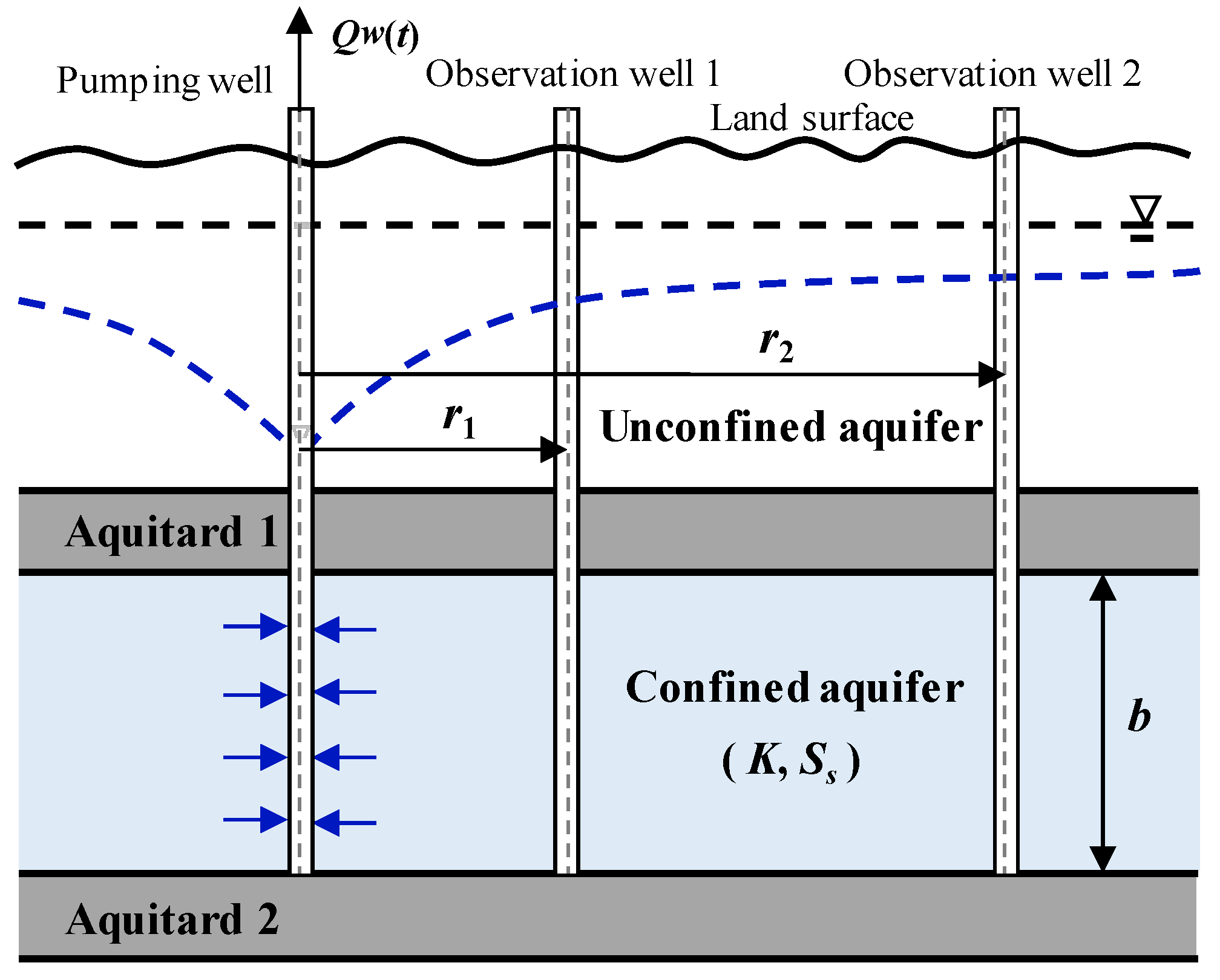
Figure 1 illustrates the proposed conceptual aquifer system. It consists of a fully penetrating pumping well located in a confined aquifer and two observation wells located at radial distances r1 and r2 from the pumping well. The assumptions used in this study are similar to those of the Theis [17] model, with the exception that the pumping rate was assumed to vary with time. Several assumptions were made for this study: (1) the confined aquifer was homogeneous, isotropic, and uniformly thick, and had an infinite extent in the radial direction; (2) the initial head of the confined aquifer was uniformly distributed throughout the system; (3) the pumping well had an infinitesimal radius, and hence, the wellbore storage was negligible; (4) groundwater flow was primarily horizontal and followed Darcy’s law; and (5) the water was removed instantaneously as the head declines. The governing equation that describes transient flow toward the fully penetrating pumping well in the confined aquifer can be written as follows [17]:
with initial condition s(r,0) = 0 and boundary conditions s(∞,t) = 0 and −Qw(t)/(2πKb), where s(r, t) denotes the aquifer drawdown at time t and radial distance r [L]; Qw(t) denotes the pumping rate at time t [L3T−1]; Ss denotes the specific storage [L−1]; K denotes the hydraulic conductivity [L1T−1]; r denotes the radial distance from the pumping well [L]; t denotes the time since the pumping started [T]; and b denotes the aquifer thickness [L].
By taking into account the initial and boundary conditions, we derived an analytical solution for the variable-rate pumping tests model. This solution is expressed as follows [27]:
where τ denotes a dummy variable of integration.
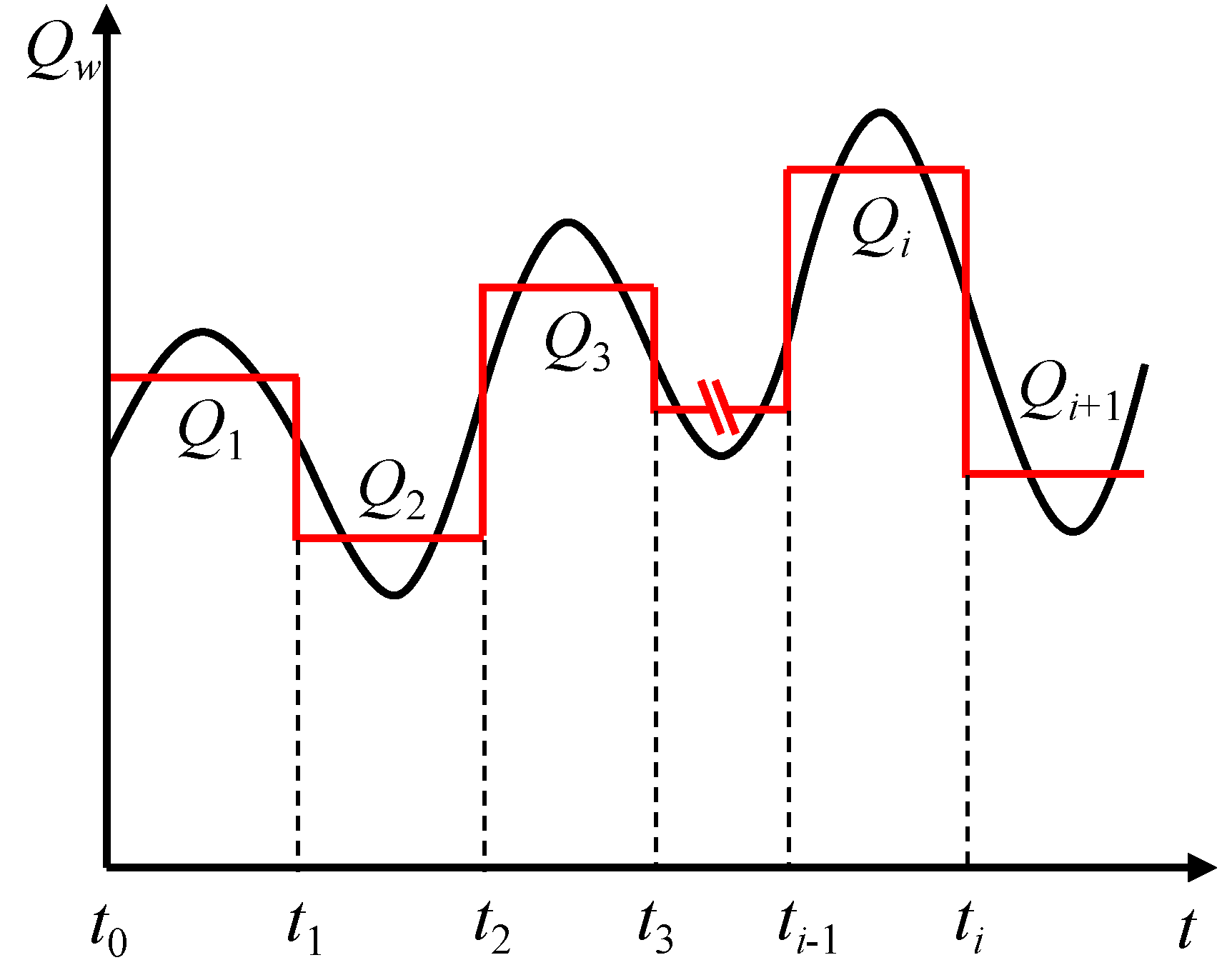
As illustrated in Figure 2, the time-varying pumping rate Qw(t) is represented by a piecewise-constant function, which was approximated by the average pumping rate Qi at each time step. Here, ti represents the inflection time at the junction between the ith and (i + 1)th step of the pumping history. It is worth noting that the initial inflection time was t0 = 0, and the initial average pumping rate was Q0 = 0. To simplify Equation (2), the following dimensionless variables for time and drawdown were introduced:
where the subscript ‘‘D’’ is the symbol of dimensionless terms hereinafter; tD and sD are the dimensionless time and dimensionless drawdown, respectively. Then, the dimensionless form of Equation (2) could be expressed as
where Qw,D(tD) = Qw(t)/Q1 denotes the dimensionless pumping rate (Q1 ≠ 0).
By discretizing Qw into n constant pumping rates (see Figure 2), Equation (4) can be rewritten as
where , , and are the increments of the dimensionless pumping rate, dimensionless inflection time, and inflection time ratio of the ith step, respectively. Note that one has t0,D = 0, φ1 = 1, and β0 = 0. Under the special condition of n = 1 (i.e., φ2 = φ3 = … = φn = 0), Equation (5) becomes a new dimensionless form of the Theis [17] solution, which is numerically equivalent to the well function.
2.2. Type Curve Method
By analyzing a field pumping test configuration, one can determine the distance r between the pumping and observation wells, as well as the thickness b of the aquifer. The pumping rates can be approximated using piecewise-constant functions by fitting the recorded data. This process enables the determination of the inflection time ti and average pumping rate Qi for each step. As a result, one can calculate the dimensionless pumping rate increment φi and inflection time ratio βi.
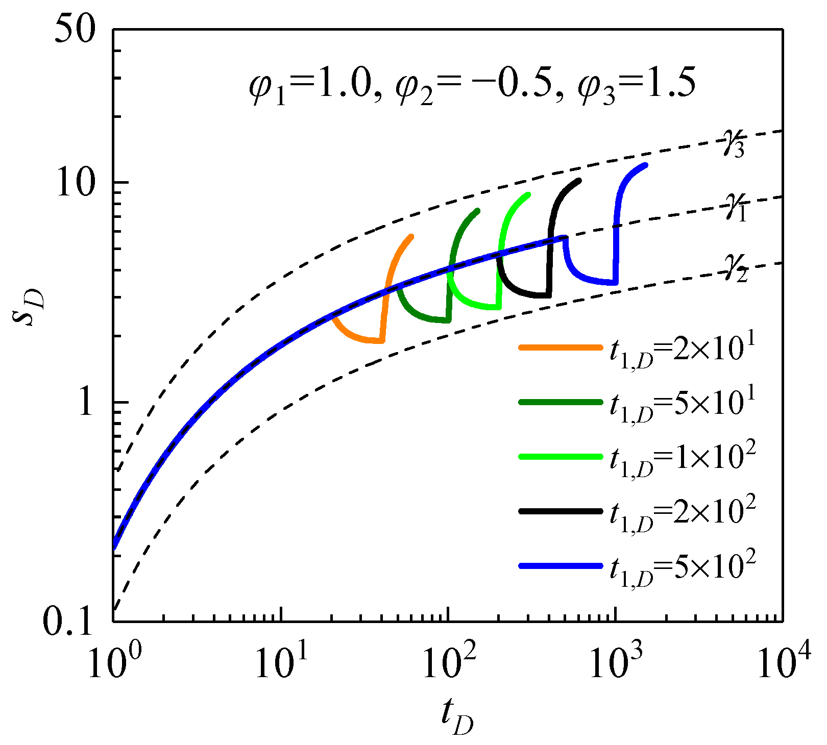
Equation (5) demonstrates that the relationship between tD and sD relies on a set of t1,D values, given βi and φi are fixed. To simplify the analysis, we considered a pumping test with three piecewise-constant pumping segments and examined the variations in sD versus tD for different t1,D values. The inflection times were set to t1 = 2 days, t2 = 4 days, and t3 = 6 days. A fully penetrating well that pumped at rates of Q1 = 4 m3/d from t0 to t1, Q2 = 2 m3/d from t1 to t2, and Q3 = 8 m3/d from t2 to t3 was considered. Thus, the involved dimensionless variables were calculated to be β1 = 1, β2 = 2, β3 = 3, φ1 = 1.0, φ2 = −0.5, and φ3 = 1.5. By substituting these values into Equation (5), we obtained a set of type curves for different first dimensionless inflection time (t1,D) values ranging from 20 to 500, as shown in Figure 3. The type curves of constant-rate pumping tests with their rates set at the first step rate (Q1), the second step rate (Q2), and the third step rate (Q3) are also depicted in this Figure 3.
The information presented in Figure 3 illustrates that the type curves associated with the first step are equivalent to the conventional Theis [17] curve (γ1). Once the pumping rate abruptly dropped to Q2 for the second step, the influence of Q2 became dominant and sD deviated from γ1, gradually approaching the lower asymptotic curve (γ2) corresponding to Qw = Q2. When the pumping rate suddenly changed from Q2 to Q3 for the third step, the type curves deviated from γ2 and approached the upper asymptotic curve γ3 in a manner that was mainly controlled by Qw = Q3. It was concluded that except for the first step, the type curves of subsequent steps will experience a sudden drawdown deviation at early and intermediate times, and gradually approach the curve of the constant-rate pumping case later on. The time corresponding to this drawdown deviation is related to the value of t1,D, and a larger t1,D will result in a later occurrence of the drawdown deviation.
In field applications, ti and Qi are determined using piecewise-constant approximations of recorded variable pumping rates. Therefore, Equation (5) shows that sD is a function of tD, and is only influenced by different values of t1,D. Taking the logarithms of both sides of tD and sD in Equation (3) results in
The constancy of the second terms on the right-hand sides of Equations (6) and (7) is evident, as they are not dependent on either the drawdown s or the time t. Consequently, when plotted on a log–log scale, the measured drawdown–time curve of s versus t exhibits a similar shape to that of the dimensionless type curve of sD versus tD. However, there is a shift of 4πKb/Q1 along the vertical (s or sD) axis and 4K/(r2Ss) along the horizontal (t or tD) axis. Equation (3) indicates that t1,D, which governs the type curve’s shape, is only linked to the confined aquifer’s hydraulic diffusivity (K/Ss) when the radial distance r and the first step’s inflection time t1 are given. Hence, the type curve method can be employed to estimate the hydraulic parameters in this study. The following outlines the new type curve method’s usage:
- (1)
- Plot the measured drawdown–time curve in a log–log graph.
- (2)
- Determine φi and βi, and prepare a series of type curves with different t1,D values in a log–log graph of the same scale as the measured curve.
- (3)
- Similar to Theis’s matching technique, match the measured drawdown–time curve with one of the type curves and choose the best matching curve.
- (4)
- Record the corresponding t1,D value, select a match point, and read the corresponding coordinates of s, t, sD, and tD.
Use Equations (8) and (9) to estimate the hydraulic parameters by substituting the above four coordinate values:
Furthermore, instead of relying on Equation (9) to calculate Ss, Ss can be determined by substituting t1,D into the following expression:
The natural geologic formations’ complex and spatially variable patterns [31,32,33] may make it difficult for real aquifer systems to satisfy all the assumptions adopted in this study, such as homogeneity, isotropy, and uniform thickness. Thus, for a specific confined aquifer, estimates of K and Ss obtained from different pumping tests or multiple observation wells of the same pumping test might differ. Variations could also be attributed to in situ pumping conditions (noise, temperature, etc.), resulting in uncertainties in the parameter estimation. Moreover, subjective errors in matching, such as the selection of matching points and reading inaccuracies, add uncertainty to parameter estimation. To mitigate the impact of such factors, most measured data should fall on the curved portion that characterizes type curves better than other parts. Furthermore, attention should be paid to the inflection point matching in each step of measured data.
While theoretically possible, determining Ss from the value of t1,D corresponding to the type curve matched with the measured data is unreliable. This is because the matching between the measured data and the type curves depends on the shapes of the type curves. These shapes differ only minimally when t1,D varies by an order of magnitude. As a result, the accuracy of this method for determining Ss is doubtful. When the measured data plot moves from one type curve to another, the determined value of K changes slightly compared with that of Ss. To eliminate doubts regarding which type curve with a t1,D value to use for matching the measured data plot, we can estimate Ss based on knowledge of the geologic conditions within an order of magnitude.
Equation (3) reveals that the dimensionless parameters introduced with respect to time and drawdown solely rely on the pumping rate record, such as the inflection time and average pumping rates of each step. As a result, different sets of drawdown data acquired from various observation wells can be processed using the type curves for a given pumping test. However, it is important to note that the new type curve method only provides a robust initial estimate of the hydraulic parameters. Thus, as discussed in the upcoming section, we first utilized the newly proposed type curve method to analyze drawdown data collected from multiple pumping tests conducted at a field site. Subsequently, we compared our estimation results with those obtained from a non-linear regression tool called PEST [30].
3. Field Application
3.1. Background
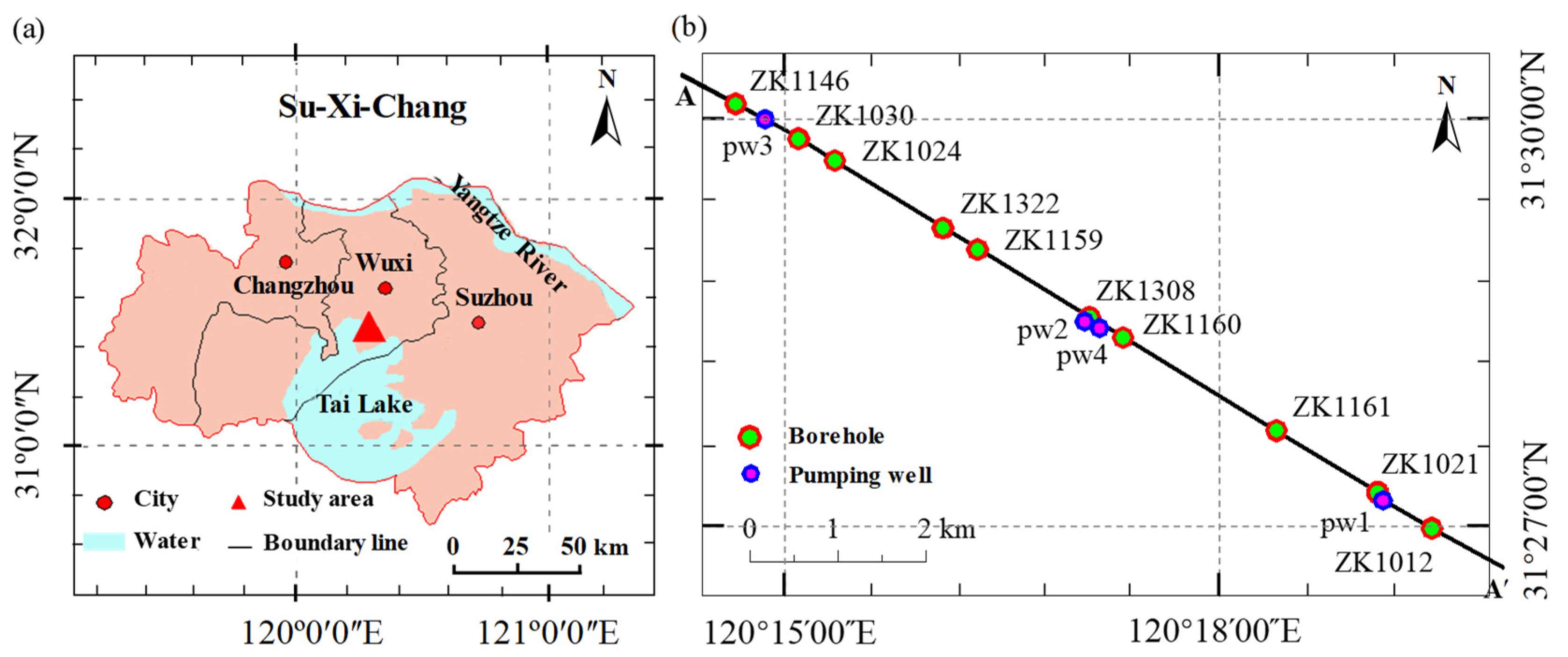
The proposed type curve method was employed to estimate the hydraulic conductivity (K) and specific storage (SS) of a confined aquifer in Wuxi City, Jiangsu Province, China. The study area was located within the plain area adjacent to Tai Lake (Figure 4a), which is characterized by relatively flat and low-lying terrain with ground elevations ranging from −1.4 m to 2.9 m. The subsurface geology comprises a multi-layered aquifer system consisting of Quaternary unconsolidated sediments, with Paleocene sandstone underlying the lower bedrock, and Pliocene–Pleistocene Holocene clay, silt, and silty sand and Holocene clay overlaying it from bottom to top.
Four pumping tests were conducted, with each test comprising one pumping well and two observation wells at the field site. The eight observation wells (ow1-1, ow1-2, ow2-1, ow2-2, ow3-1, ow3-2, ow4-1, and ow4-2), as well as the four pumping wells (pw1, pw2, pw3, and pw4) selected for analysis in this study fully penetrated the aquifers being tested. In all pumping tests, one observation well was positioned at a distance of 5 m from the pumping well, while the other was placed 15 m away.
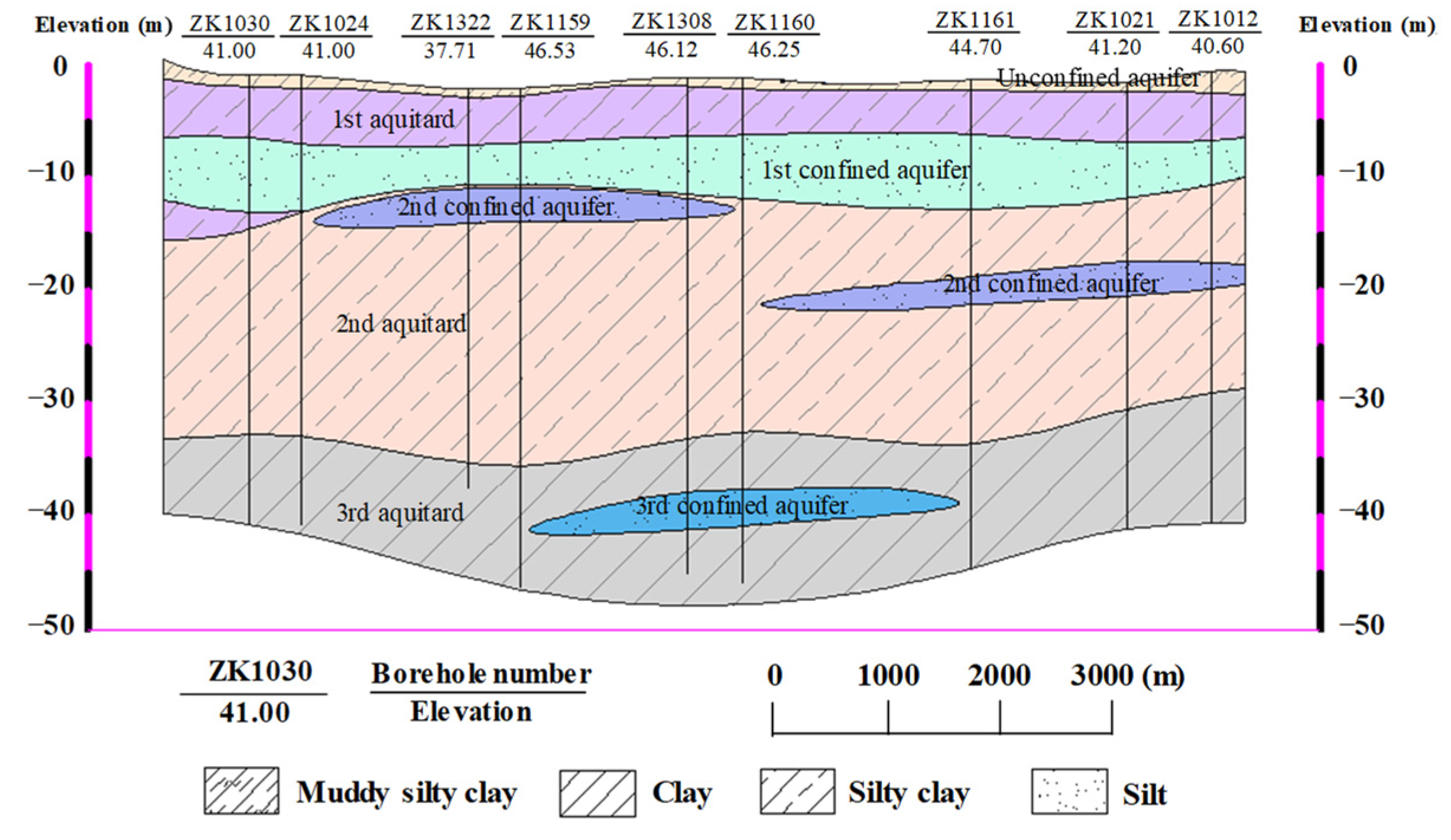
Figure 4b depicts the boreholes and pumping wells in the study area, where A–A′ represents the survey line. The hydrogeological profile obtained from borehole data along A–A′ revealed that the aquifer system in this study area was composed of four aquifers and three aquitards (Figure 5). The sandy silt layers presented in the middle and lower parts of the strata comprised the first, second, and third confined aquifers. These aquifers were recharged through horizontal infiltration of surface water and vertical leakage from the upper unconfined, and discharged through lateral runoff, vertical leakage, and artificial exploitation. The clayey layers overlying and underlying the aquifers served as aquitards with relatively low permeability. From top to bottom, these were identified as the first, second, and third aquitards. Lithological information showed that the void ratio (e) values of the first and second confined aquifers were 0.808 and 0.746, respectively.
The objective of this study was to analyze the hydraulic properties of the first and second confined aquifers. The first confined aquifer, which ranged in thickness from 1.00 m to 12.60 m, was composed of silt with interbedded silty sand and silty clay, and it had a wider horizontal distribution and greater thickness compared with the second confined aquifer. On the other hand, the second confined aquifer, which ranged in thickness from 1.30 m to 3.40 m, consisted of silt with partly silty sand and silty clay deposits. It can be seen that the second confined aquifer was discontinuous in space, and was shown as two parts with the same lithology in Figure 5. Since the lateral range of each part was greater than 3000 m, both parts can be treated as independent hydrogeological units for analysis.
3.2. Analysis of In Situ Pumping Test
At the field site, four pumping tests were conducted within the first and second confined aquifers. The first and second pumping tests were carried out in the second confined aquifer while the third and fourth pumping tests were conducted in the first confined aquifer. Based on the borehole logs of pumping and observation wells and other logs of boreholes, the aquifer thicknesses of the first to fourth pumping tests were determined to be 2.5, 5.9, 4.1, and 7.0 m, respectively.
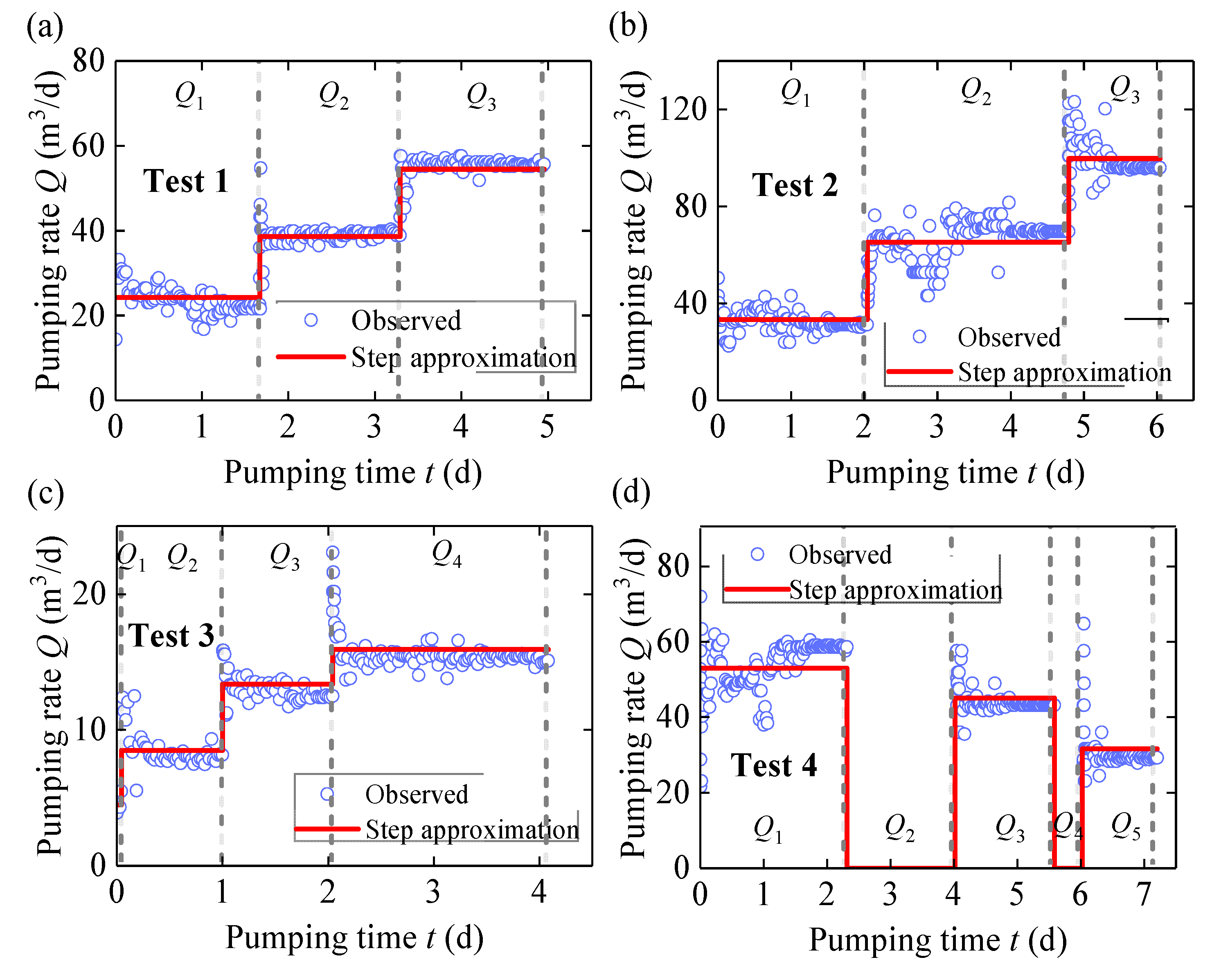
The total durations of the first to fourth pumping tests were 7140, 8700, 5880, and 10,380 min, respectively. For each test, the pumping rate of the pumping well and water level of the two observation wells were recorded at 1, 2, 3, 4, 5, 6, 8, 10, 15, 20, 25, 30, 40, 50, 60, 80, 100, and 120 min after the start of each step, and then every 30 min until the water level in each step reached a steady state. Pumping rate records (Figure 6) from the four pumping wells and associated drawdown records of eight observation wells (Figure 7) were used in the type curve analysis.
Figure 6 illustrates that each pumping test was conducted in three to five steps, with each step maintaining a constant pumping rate. Tests 1 and 2 had a three-step pumping rate change during their durations, while test 3 had a four-step change, including a short step at the beginning. The fourth test underwent five-step pumping, which included two instances where the pumping rate was abruptly reduced to zero. Although the proposed type curve method can be utilized to analyze the recovery data during shutdown periods, only the observed data from the pumping period of the fourth test were used to estimate hydraulic parameters, as there was no drawdown record during the shutdown period.
To demonstrate the type curve analysis, we utilized the observed drawdown data collected from the first observation well (ow1-1) in pumping test 1, which was conducted within the second confined aquifer and lasted for 7140 min (about 4.96 days). The record of corresponding pumping rates was approximated into three continuous constant-rate segments, as shown in Figure 6a. The corresponding inflection time points were determined to be t1 = 1.67 days, t2 = 3.29 days, and t3 = 4.96 days, with time intervals corresponding to the three steps being 1.67, 1.63, and 1.67 days, respectively. Additionally, the average pumping rates of the three steps were Q1 = 24.27 m3/d, Q2 = 38.67 m3/d, and Q3 = 54.47 m3/d.
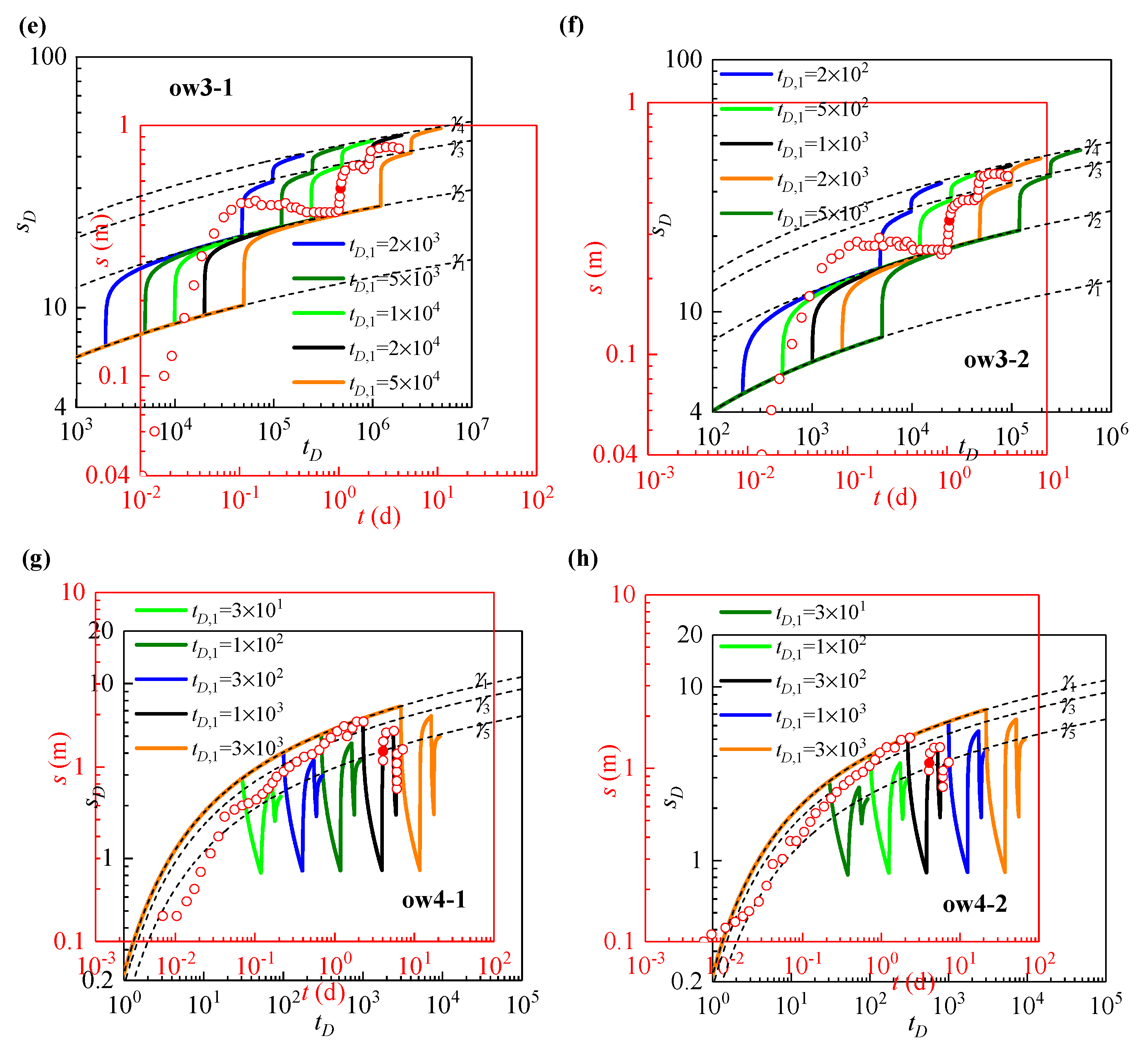
Using the pumping rate record, we calculated the inflection time ratio values to be β1 = t1/t1 = 1.00, β2 = t2/t1 = 1.97, and β3 = t3/t1 = 2.97. The dimensionless pumping rate increments for each step were φ1 = 1.00, φ2 = (Q2 − Q1)/Q1 = 0.59, and φ3 = (Q3 − Q2)/Q1 = 0.65. We substituted these values into Equation (5) to derive a series of type curves that were functions of t1,D values, ranging from 100 to 2000, as depicted in Figure 7a. By matching the measured time–drawdown data to the type curves on a log–log graph, we found that the type curve with t1,D = 500 provided the best match, as shown in Figure 7a. We selected a matching point with the coordinates of t = 1.74 days, s = 6.53 m, tD = 516.72, and sD = 7.04 for the parameter estimation. By substituting these values into Equations (8) and (9), we obtained K = (7.04 × 24.27)/(4 × π × 2.5 × 6.53) = 0.83 m/d and Ss = (7.04 × 24.27 × 1.74)/(π × 2.5 × 6.53 × 52 × 516.72) = 4.47 × 10⁻⁴ m−1.
Figure 7b displays the matching results of ow1-2 in a comparable fashion. It is important to highlight that when estimating the hydraulic parameters of the second confined aquifer using the measured data of ow1-2, the distance between ow1-2 and pw1 (i.e., r = 15 m) was used as a substitute. The matching point, which is represented by a red solid dot in Figure 7b, was identified at the coordinates t = 1.79 days, s = 5.53 m, tD = 213.26, and sD = 6.02. By substituting these coordinate values into Equations (8) and (9), we obtained K = 0.84 m/d and Ss = 1.26 × 10⁻⁴ m−1. The type curve matching results for the other three pumping tests are presented in Figure 7c–h, following a similar process as that for pumping test 1. The values of the t1,D, coordinate values of the matching points, and estimated values of K and Ss for the four pumping tests are listed in Table 1.
4. Discussion
Section 2.2 highlights the uncertainties related to parameter estimation using the type curve method. This method is subject to subjective matching errors, such as the selection of matching points and reading errors, which are inevitable and can only be minimized through the experience of operators. To evaluate the reliability of the hydraulic parameters estimated using the type curve method, we utilized PEST, which is a model-independent parameter estimation program that is highly versatile [30].
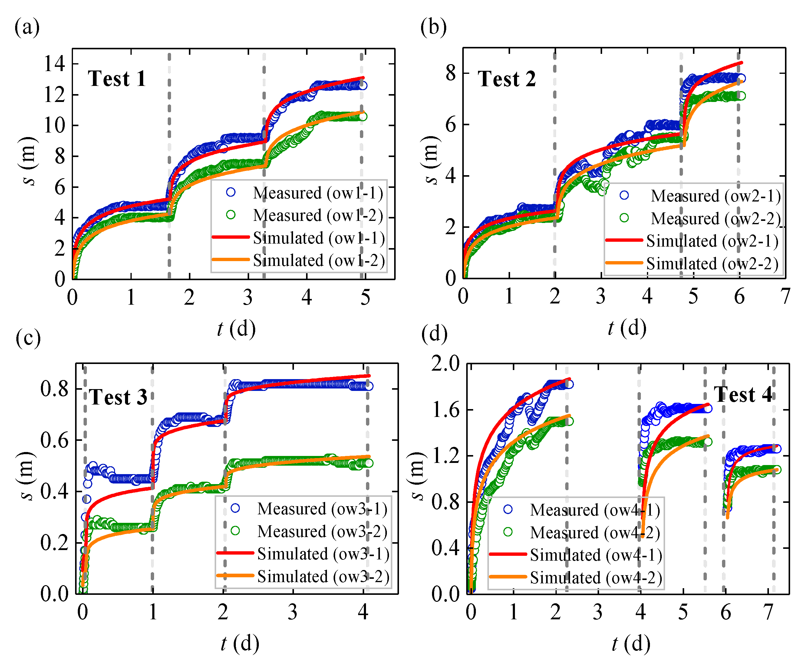
According to Doherty [30], selecting a reasonable initial parameter value is crucial when using PEST with the Levenberg–Marquardt algorithm. The initial value should be close to the optimized value to enhance the optimization efficiency. In this study, we used the hydraulic parameters obtained through the type curve method as the initial guess for automatic estimation by coupling the analytical solution, i.e., Equation (5), with PEST. Figure 8 displays a comparison between the simulated and observed drawdowns for each pumping test, and the estimated parameters are summarized in Table 2.
To compare the parameter estimation results for different observation wells, test sites, and aquifers, the sum of the squared weight residual provided by PEST cannot be used uniformly. Therefore, we utilized the Nash–Sutcliffe coefficient (CE) [34] to conduct a quantitative analysis of the validity of estimated parameters. This was done mainly by comparing the standard deviation between the measured and simulated drawdowns. CE was calculated using the following formula [34]:
where CE denotes the Nash–Sutcliffe coefficient; nu denotes the number of measured drawdowns; sp,i and sm,i denote simulation drawdowns and measured drawdowns, respectively; and smc denotes the average value of measured drawdowns. According to Nash and Sutcliffe [34], a higher CE value indicates that the simulated and measured data are more closely aligned. When the simulated and measured data match perfectly, the CE value is 1. Moreover, if CE exceeds the threshold of 0.5, it suggests that the deviation between the simulated and measured data is acceptable, which ameans that the estimated parameters can be considered reliable.
Table 2 indicates that all eight observation wells had CE values exceeding 0.5, implying that approximating the time-varying pumping rates using a piecewise-constant function was feasible and that the estimates of the hydraulic parameters K and Ss were reasonable. Notably, pumping tests 1 and 2 had higher CE values than the other two tests, indicating that the reliability of the K and Ss estimates of tests 1 and 2 in the second confined aquifer was higher than that of tests 3 and 4 in the first confined aquifer. It is worth mentioning that although the CE value for pumping test 3 exceeded 0.90, there was a significant visible difference between the simulated and measured drawdowns (Figure 8c). The primary reason for this disparity could be attributed to the fact that the early period of pumping exhibited a continuous decrease in pumping rate over time, which did not perfectly align with the assumption of piecewise-constant pumping (Figure 6c).
It is noteworthy that the piecewise-constant rate pumping test in this study differed from the step-drawdown test [21,35], which involves the sequential increase of pumping rate in several intervals. The piecewise-constant rate pumping test does not have such a continuous increase restriction, and thus, the newly proposed type curve method can be applied to analyze pumping tests with arbitrary step rate changes, especially those with unexpected pumping shutdowns (e.g., pumping test 4). It was observed that pumping test 4 involved three instances of starting and stopping pumping throughout the test, with significantly lower CE values compared with the other three tests. This discrepancy between the simulated and measured drawdowns could be attributed to the two shutdowns during the test, as shown in Figure 6d. On the one hand, the pumping equipment may have caused unnecessary mechanical losses each time it was started. On the other hand, the abrupt fluctuations in aquifer water level caused by the starting and stopping of the pumping may have resulted in turbulence loss, which is a potential factor that cannot be ignored.
As shown in Table 2, the confidence intervals for the K estimates were generally narrow, indicating a high degree of confidence in these estimates. Similarly, the Ss estimates were also associated with narrow confidence intervals, even though those corresponding to pumping tests 3 and 4 were slightly wider. The differences between the K or Ss estimates from various observation wells for the same pumping test may be attributed to the nonuniform thickness of the confined aquifer and spatial heterogeneity, which are commonly found in nature [31,32,33]. The influence of aquifer boundaries on parameter estimation may be ignored, as even the relatively small second confined aquifer had a lateral boundary range of 3000 m. Furthermore, for a specific pumping test, the difference in Ss is typically greater than K, suggesting relatively higher heterogeneity in Ss than K. Finally, it is noteworthy that the two aquifers of interest had noticeably different K and Ss parameter estimates.
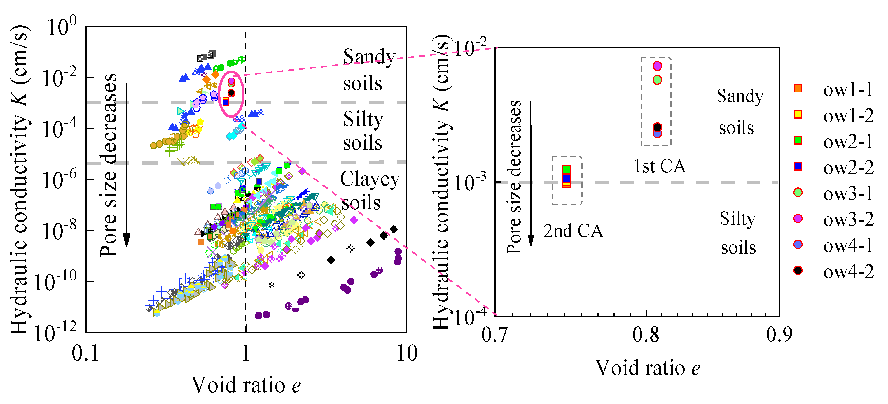
Comparing Table 1 and Table 2 revealed that the K and Ss values obtained from the new type curve method were comparable to those provided by PEST, underscoring the reliability of this new method. To further validate the calibrated K estimates, a comparison was made with compiled experimental results reported in Ren and Santamarina [36], as shown in Figure 9.
Ren and Santamarina [36] noted that for a given void ratio, the range of K depended on the soil types (e.g., sandy, silty, and clayed soils). In this study, the field investigation confirmed that the first and second confined aquifers primarily consisted of silty deposits that were partly silty sand and silty clay with void ratios of 0.808 and 0.746, respectively. By combining the void ratios of both confined aquifers and the corresponding K values calibrated using PEST (Figure 9), we found that the estimated K values for the first confined aquifer fell within the “Sandy” region, while those for the second confined aquifer fell on both sides of the dividing line between the “Sandy” and “Silty” regions. This suggests that the K estimates aligned well with the lithological data. The geometric means of K and Ss were also calculated, yielding values of 6.62 m/d and 3.16 × 10⁻⁵ m−1 for the first confined aquifer and 0.92 m/d and 2.34 × 10⁻⁴ m−1 for the second confined aquifer.
5. Conclusions
This study employed type curve analysis to investigate variable-rate pumping tests conducted in a confined aquifer by assuming the variability to be a piecewise-constant function. Based on this assumption, a new type curve method was proposed to estimate the hydraulic conductivity (K) and specific storage (Ss). The proposed method was then applied to interpret field pumping tests carried out in an aquifer system located in Wuxi City, Jiangsu Province, China. The main conclusions drawn from this study are as follows:
- (1)
- The study introduced a new dimensionless transformation formula to simplify the analytical solution of variable-rate pumping tests, and a piecewise-constant function was further used to approximate the time-varying pumping rate records. Type curve analyses revealed that the time–drawdown curve of the first step was consistent with the Theis curve. However, the type curves of the subsequent steps deviated from the Theis curve and were associated with the first dimensionless inflection time (t1,D), which depended on the K and Ss of the confined aquifers. A large t1,D resulted in a faster time for a sudden turn in the drawdown.
- (2)
- A new type curve method was proposed to handle situations where the real pumping rate varies in a complicated pattern over time. One unique feature of this method is that the type curves depend on the pumping conditions rather than the observation conditions, making it applicable to drawdown data collected from various observation wells during a single pumping test. Furthermore, this new method could also be used to analyze recovery drawdown data by setting a zero pumping rate value for the corresponding shutdown period.
- (3)
- The hydraulic conductivity (K) and specific storage (Ss) of the first and second confined aquifers at the field site were estimated using the pumping rate and drawdown records from four real pumping tests. The estimation results showed that the hydraulic parameters obtained from the newly proposed type curve method were close to the calibrated results reported by PEST, indicating the reliability and robustness of this new method. Moreover, the K estimates were further verified by comparing them with lithology-based results. The geometric means of K and Ss were 6.62 m/d and 3.16 × 10⁻⁵ m−1 for the first confined aquifer and 0.92 m/d and 2.34 × 10⁻⁴ m−1 for the second confined aquifer.
- (4)
- The field pumping test results showed that the actual pumping rate may have an uncontrollable and short-duration decreasing trend at the early times of each step, resulting in uncertainty in the evaluation of aquifer hydraulic parameters. In addition, the heterogeneity of natural aquifers and the non-uniformity of their thickness also led to differences in the estimated hydraulic parameters of different observation wells in the same pumping test. Future studies will focus on characterizing the heterogeneity of aquifer systems from multiple pumping test data based on more realistic and refined pumping models.
Author Contributions
Methodology, Y.L. and Z.Z.; Software, Y.L.; Validation, Y.L., C.Z. and Z.D.; Formal analysis, Y.L., Z.Z., C.Z. and Z.D.; Investigation, Z.Z. and C.Z.; Writing—original draft, Y.L. All authors have read and agreed to the published version of the manuscript.
Funding
The research was financially supported by the National Natural Science Foundation of China (grant no. 41572209).
Data Availability Statement
The data presented in this study are available on request from the corresponding author.
Conflicts of Interest
The authors declare no conflict of interest.
References
- Banks, D.; Odling, N.E.; Skarphagen, H.; Rohr-Torp, E. Permeability and stress in crystalline rocks. Terra Nova 1996, 8, 223–235. [Google Scholar] [CrossRef]
- Liu, J.; Zhao, Y.; Tan, T.; Zhang, L.; Zhu, S.; Xu, F. Evolution and modeling of mine water inflow and hazard characteristics in southern coalfields of China: A case of Meitanba mine. Int. J. Min. Sci. Technol. 2022, 32, 513–524. [Google Scholar] [CrossRef]
- Manoutsoglou, E.; Lazos, I.; Steiakakis, E.; Vafeidis, A. The Geomorphological and Geological Structure of the Samaria Gorge, Crete, Greece-Geological Models Comprehensive Review and the Link with the Geomorphological Evolution. Appl. Sci. 2022, 12, 10670. [Google Scholar] [CrossRef]
- Stober, I.; Bucher, K. Origin of salinity of deep groundwater in crystalline rocks. Terra Nova 1999, 11, 181–185. [Google Scholar] [CrossRef]
- Yuan, Z.; Zhao, J.; Li, S.; Jiang, Z.; Huang, F.A. Unified Solution for Surrounding Rock of Roadway Considering Seepage, Dilatancy, Strain-Softening and Intermediate Principal Stress. Sustainability 2022, 14, 8099. [Google Scholar] [CrossRef]
- Zhao, Y.; Liu, Q.; Zhang, C.; Liao, J.; Lin, H.; Wang, Y. Coupled seepage-damage effect in fractured rock masses: Model development and a case study. Int. J. Rock Mech. Min. 2021, 144, 104822. [Google Scholar] [CrossRef]
- Zhao, Y.; Luo, S.; Wang, Y.; Wang, W.; Zhang, L.; Wan, W. Numerical Analysis of Karst Water Inrush and a Criterion for Establishing the Width of Water-resistant Rock Pillars. Mine Water Environ. 2017, 36, 508–519. [Google Scholar] [CrossRef]
- Chapuis, R.P.; Aubertin, M. On the use of the Kozeny–Carman equation to predict the hydraulic conductivity of soils. Can. Geotech. J. 2003, 40, 616–628. [Google Scholar] [CrossRef]
- Ren, X.; Zhao, Y.; Deng, Q.; Li, D.; Wang, D. A relation of hydraulic conductivity-Void ratio for soils based on Kozeny-carman equation. Eng. Geol. 2016, 213, 89–97. [Google Scholar] [CrossRef]
- Gallage, C.; Kodikara, J.; Uchimura, T. Laboratory measurement of hydraulic conductivity functions of two unsaturated sandy soils during drying and wetting processes. Soils Found. 2013, 53, 417–430. [Google Scholar] [CrossRef]
- Masrouri, F.; Bicalho, K.V.; Kawai, K. Laboratory Hydraulic Testing in Unsaturated Soils. Geotech. Geol. Eng. 2008, 26, 691–704. [Google Scholar] [CrossRef]
- Abdalla, F.; Mubarek, K. Assessment of well performance criteria and aquifer characteristics using step-drawdown tests and hydrogeochemical data, west of Qena area, Egypt. J. Afr. Earth. Sci. 2018, 138, 336–347. [Google Scholar] [CrossRef]
- Hendrayanto; Kosugi, K.I.; Mizuyama, T. Field Determination of Unsaturated Hydraulic Conductivity of Forest Soils. J. For. Res. 1998, 3, 11–17. [Google Scholar] [CrossRef]
- Neuman, S.P.; Witherspoon, P.A. Field determination of the hydraulic properties of leaky multiple aquifer systems. Water Resour. Res. 1972, 8, 1284–1298. [Google Scholar] [CrossRef]
- Sethi, R. A dual-well step drawdown method for the estimation of linear and non-linear flow parameters and wellbore skin factor in confined aquifer systems. J. Hydrol. 2011, 400, 187–194. [Google Scholar] [CrossRef]
- Butt, M.A.; Mcelwee, C.D. Aquifer-Parameter Evaluation from Variable-Rate Pumping Tests Using Convolution and Sensitivity Analysis. Groundwater 1985, 23, 212–219. [Google Scholar] [CrossRef]
- Theis, C.V. The relation between the lowering of the Piezometric surface and the rate and duration of discharge of a well using ground-water storage. EOS Trans. Am. Geophys. Union 1935, 16, 519–524. [Google Scholar] [CrossRef]
- Cooper, H.H.; Jacob, C.E. A generalized graphical method for evaluating formation constants and summarizing well-field history. EOS Trans. Am. Geophys. Union 1946, 27, 526–534. [Google Scholar] [CrossRef]
- Hantush, M.S. Nonsteady Flow to Flowing Wells in Leaky Aquifers. J. Geophys. Res. 1959, 64, 1043–1052. [Google Scholar] [CrossRef]
- Neuman, S.P. Theory of Flow in Unconfined Aquifers Considering Delayed Response of the Water Table. Water Resour. Res. 1972, 8, 1031–1045. [Google Scholar] [CrossRef]
- Rorabaugh, M. Graphical and theoretical analysis of step-drawdown test of artesian well. Proc. Am. Soc. Civ. Eng. 1953, 79, 1–23. [Google Scholar]
- Sen, Z.; Altunkaynak, A. Variable discharge type curve solutions for confined aquifers. J. Am. Water Resour. Assoc. 2004, 40, 1189–1196. [Google Scholar] [CrossRef]
- Butler, J.J.; McElwee, C.D. Variable-rate pumping tests for radially symmetric nonuniform aquifers. Water Resour. Res. 1990, 26, 291–306. [Google Scholar] [CrossRef]
- Hantush, M.S. Drawdown around Wells of Variable Discharge. J. Geophys. Res. 1964, 69, 4221–4235. [Google Scholar] [CrossRef]
- Singh, S.K. Well Loss Estimation: Variable Pumping Replacing Step Drawdown Test. J. Hydraul. Eng. 2002, 128, 343–348. [Google Scholar] [CrossRef]
- Wen, Z.; Zhan, H.; Wang, Q.; Liang, X.; Ma, T.; Chen, C. Well hydraulics in pumping tests with exponentially decayed rates of abstraction in confined aquifers. J. Hydrol. 2017, 548, 40–45. [Google Scholar] [CrossRef]
- Zhang, G. Type curve and numerical solutions for estimation of Transmissivity and Storage coefficient with variable discharge condition. J. Hydrol. 2013, 476, 345–351. [Google Scholar] [CrossRef]
- Zhuang, C.; Zhou, Z.; Zhan, H.; Wang, J.; Li, Y. New graphical methods for estimating aquifer hydraulic parameters using pumping tests with exponentially decreasing rates. Hydrol. Process 2019, 33, 2314–2322. [Google Scholar] [CrossRef]
- Luo, N.; Zhanfeng, Z.; Walter, A.I.; Steven, J.B. Comparative study of transient hydraulic tomography with varying parameterizations and zonations: Laboratory sandbox investigation. J. Hydrol. 2017, 554, 758–779. [Google Scholar] [CrossRef]
- Doherty, J. PEST: Model Independent Parameter Estimation; Watermark Computing: Corinda, Australia, 2008. [Google Scholar]
- Copty, N.K.; Trinchero, P.; Sanchez-Vila, X.; Sarioglu, M.S.; Findikakis, A.N. Influence of heterogeneity on the interpretation of pumping test data in leaky aquifers. Water Resour. Res. 2008, 44, 2276–2283. [Google Scholar] [CrossRef]
- Demir, M.T.; Copty, N.K.; Trinchero, P.; Sanchez-Vila, X. Bayesian Estimation of the Transmissivity Spatial Structure from Pumping Test Data. Adv. Water Resour. 2017, 104, 174–182. [Google Scholar] [CrossRef]
- Sudicky, E.A.; Illman, W.A.; Goltz, I.K.; Adams, J.J.; Mclaren, R.G. Heterogeneity in hydraulic conductivity and its role on the macroscale transport of a solute plume: From measurements to a practical application of stochastic flow and transport theory. Water Resour. Res. 2010, 46, 489–496. [Google Scholar] [CrossRef]
- Nash, J.; Sutcliffe, J. River flow forecasting through conceptual models: I. A discussion of principles. J. Hydrol. 1970, 10, 282–290. [Google Scholar] [CrossRef]
- Chen, C.; Tao, Q.; Wen, Z.; Wörman, A.; Jakada, H. Step-drawdown test for identifying aquifer and well loss parameters in a partially penetrating well with irregular (non-linear increasing) pumping rates. J. Hydrol. 2022, 614, 128652. [Google Scholar] [CrossRef]
- Ren, X.W.; Santamarina, J.C. The hydraulic conductivity of sediments: A pore size perspective. Eng. Geol. 2018, 233, 48–54. [Google Scholar] [CrossRef]
Figure 1.
Conceptual model of a confined aquifer system with a pumping well and two observation wells. Qw represents the time-varying pumping rate; K and Ss represent the hydraulic conductivity and specific storage of the confined aquifer, respectively; and r1 and r2 represent the radial distances between the two observation wells and the pumping well, respectively.

Figure 2.
Approximation of the time-varying observed pumping rates (black curve) using a piecewise-constant function (red curve). Qi represents the average pumping rate of the ith step from ti−1 to ti.
Figure 2.
Approximation of the time-varying observed pumping rates (black curve) using a piecewise-constant function (red curve). Qi represents the average pumping rate of the ith step from ti−1 to ti.

Figure 3.
Type curves of dimensionless time tD versus dimensionless drawdown sD with a series of t1,D values. γ1 denotes the Theis curve; γ2 and γ3 are the asymptotic curves for the type curves in the second and third steps, respectively.
Figure 3.
Type curves of dimensionless time tD versus dimensionless drawdown sD with a series of t1,D values. γ1 denotes the Theis curve; γ2 and γ3 are the asymptotic curves for the type curves in the second and third steps, respectively.

Figure 4.
The field site location for the pumping tests. (a) The location of the study area; (b) the locations of boreholes and pumping wells. A–A′ denotes the survey line.
Figure 4.
The field site location for the pumping tests. (a) The location of the study area; (b) the locations of boreholes and pumping wells. A–A′ denotes the survey line.

Figure 5.
The hydrogeological profile obtained along the survey line A–A.

Figure 6.
Observed time-varying pumping rates (blue points) and corresponding piecewise-constant or step approximation (red line). (a) First pumping test; (b) Second pumping test; (c) Third pumping test; (d) Fourth pumping test. Qi denotes the average pumping rate of the ith step. Tests 1 and 2 were conducted in the 2nd confined aquifer, and tests 3 and 4 were conducted in the 1st confined aquifer.

Figure 7.
Matching the scattered points of pumping time (t) versus measured drawdown (s) with the type curves (tD versus sD) depending on different t1,D values. (a,b) Observation wells 1 and 2 for the first pumping test; (c,d) Observation wells 1 and 2 for the second pumping test; (e,f) Observation wells 1 and 2 for the third pumping test; (g,h) Observation wells 1 and 2 for the fourth pumping test. Red circle and red solid dot denote the measured drawdown and matching point selected for the parameter estimation, respectively.


Figure 8.
Simulated drawdowns (scattered points) and measured drawdowns (solid lines) of four pumping tests. (a) First pumping test; (b) Second pumping test; (c) Third pumping test; (d) Fourth pumping test. Each test result includes the measured drawdown data of two observation wells, where the blue points represent the drawdowns of observation well 1, and the green points represent the drawdowns of observation well 2.

Figure 9.
Comparison of the estimated K in this study with compiled experimental results adapted with permission from Ren and Santamarina [36], Engineering Geology, published by Elsevier, 2018. CA represents a confined aquifer.
Figure 9.
Comparison of the estimated K in this study with compiled experimental results adapted with permission from Ren and Santamarina [36], Engineering Geology, published by Elsevier, 2018. CA represents a confined aquifer.


Table 1.
Hydraulic conductivity K (m/d) and specific storage Ss (×10−4 m−1), as estimated using type curve analysis of pumping tests with piecewise-constant rates.
Table 1.
Hydraulic conductivity K (m/d) and specific storage Ss (×10−4 m−1), as estimated using type curve analysis of pumping tests with piecewise-constant rates.
| Test No. (Aquifer) | Obs. Well | t1,D | Coordinate Values | K | Ss | |||
|---|---|---|---|---|---|---|---|---|
| tD | sD | t (d) | s (m) | |||||
| 1 (2nd CA *) | ow1-1 | 500 | 516.72 | 7.04 | 1.74 | 6.53 | 0.83 | 4.47 |
| ow1-2 | 200 | 213.26 | 6.02 | 1.79 | 5.53 | 0.84 | 1.26 | |
| 2 (2nd CA) | ow2-1 | 1000 | 1020.38 | 8.73 | 2.13 | 3.66 | 1.07 | 3.58 |
| ow2-2 | 200 | 217.55 | 7.05 | 2.27 | 3.55 | 0.89 | 1.66 | |
| 3 (1st CA) | ow3-1 | 20,000 | 481,359.64 | 30.96 | 1.06 | 0.54 | 4.98 | 0.02 |
| ow3-2 | 1000 | 24,185.94 | 23.10 | 1.06 | 0.34 | 5.90 | 0.05 | |
| 4 (1st CA) | ow4-1 | 1000 | 1754.08 | 4.11 | 4.06 | 1.23 | 2.01 | 7.47 |
| ow4-2 | 300 | 569.65 | 3.56 | 4.07 | 1.07 | 2.01 | 2.55 | |
Note: * CA denotes confined aquifer.
Table 2.
PEST-estimated values of K and Ss and Nash–Sutcliffe coefficients (CE) for each pumping test.
Table 2.
PEST-estimated values of K and Ss and Nash–Sutcliffe coefficients (CE) for each pumping test.
| Test No. (Aquifer) | Observation Well | K (m/d) | Ss (×10−4 m−1) | CE |
|---|---|---|---|---|
| 1 | ow1-1 | 0.84 [0.81,0.87] a | 4.28 [3.67,4.99] | 0.993 |
| (2nd CA *) | ow1-2 | 0.87 [0.83,0.91] | 1.22 [1.03,1.44] | 0.988 |
| 2 | ow2-1 | 1.07 [0.99,1.14] | 3.75 [2.66,5.28] | 0.973 |
| (2nd CA) | ow2-2 | 0.92 [0.85,0.98] | 1.53 [1.17,2.01] | 0.972 |
| 3 | ow3-1 | 4.96 [4.30,5.62] | 0.02 [0.004,0.08] | 0.933 |
| (1st CA) | ow3-2 | 6.28 [5.73,6.83] | 0.04 [0.02,0.08] | 0.958 |
| 4 | ow4-1 | 1.98 [1.85,2.11] | 8.85 [6.63,11.81] | 0.819 |
| (1st CA) | ow4-2 | 2.20 [2.03,2.37] | 1.78 [1.30,2.43] | 0.743 |
Note: a Values inside the bracket represent the 95% confidence intervals reported. * CA denotes confined aquifer
Disclaimer/Publisher’s Note: The statements, opinions and data contained in all publications are solely those of the individual author(s) and contributor(s) and not of MDPI and/or the editor(s). MDPI and/or the editor(s) disclaim responsibility for any injury to people or property resulting from any ideas, methods, instructions or products referred to in the content. |
© 2023 by the authors. Licensee MDPI, Basel, Switzerland. This article is an open access article distributed under the terms and conditions of the Creative Commons Attribution (CC BY) license (https://creativecommons.org/licenses/by/4.0/).
Share and Cite
MDPI and ACS Style
Li, Y.; Zhou, Z.; Zhuang, C.; Dou, Z. Estimating Hydraulic Parameters of Aquifers Using Type Curve Analysis of Pumping Tests with Piecewise-Constant Rates. Water 2023, 15, 1661. https://doi.org/10.3390/w15091661
AMA Style
Li Y, Zhou Z, Zhuang C, Dou Z. Estimating Hydraulic Parameters of Aquifers Using Type Curve Analysis of Pumping Tests with Piecewise-Constant Rates. Water. 2023; 15(9):1661. https://doi.org/10.3390/w15091661
Chicago/Turabian StyleLi, Yabing, Zhifang Zhou, Chao Zhuang, and Zhi Dou. 2023. "Estimating Hydraulic Parameters of Aquifers Using Type Curve Analysis of Pumping Tests with Piecewise-Constant Rates" Water 15, no. 9: 1661. https://doi.org/10.3390/w15091661
Note that from the first issue of 2016, this journal uses article numbers instead of page numbers. See further details here.