Pipeline-Burst Detection on Imbalanced Data for Water Supply Networks

Abstract

Data-driven methods based on samples from a supervisory control and data acquisition system have been widely applied in water-supply-network burst detection to save unexpected economic and labor costs. However, the class imbalance problem in actual on-site monitoring needs to be revised to improve the performance of data-driven methods. In this study, we proposed a domain adaptation method to generate minor-category samples (pipeline-burst samples in general) of arbitrary pipe networks utilizing theoretical hydraulic models. The proposed method transferred pipeline-burst data generated from a random water supply network with theoretical hydraulic models to an actual imbalanced dataset. Accordingly, we established a machine learning model exploring a mapping matrix between two domains for minority-category data transfer. The experimental validation first verified the effectiveness and reliability of the proposed method between two customized water supply networks in terms of their bust recognition accuracy, model parameter sensitivity and time efficiency. Then, an actual monitoring dataset from a working water supply network was used to prove the suitability and compatibility of the proposed method. A bust-point location method was also provided based on the detection results of pipeline-bursting events. The validations show the superiority of our proposed approach for the imbalance data problem in pipe burst detection.

1. Introduction

A water pipeline-burst event may cause water pollution, energy waste, urban infrastructure invalidity, etc., seriously decreasing water supply quality and efficiency. Thus, burst accident identification is a critical concern in public service and academic research [1,2].

Data-driven methods have attracted more attention in current research than traditional pipeline-burst identification methods based on manual observation and experience [3]. The data-driven approach employs monitoring data [4,5], such as water pressure, water flow, etc., to a water supply network to detect pipeline-burst accidents by mathematical models [6]. These methods are based on historical data instead of specific in-depth prior knowledge [7], demonstrating significant advantages in expenditure, time and labor [2,5,8]. They indicate excellent potential for fast and flexible anomaly detection [9,10]. With the support of supervisory control and data acquisition (SCADA) systems, data-driven methods are now widely used in pipeline-burst detection of water supply networks [11]. Specifically, the water pipe pressures obtained from several onsite pressure gauges are the favorite data basis for machine learning models in a low-cost burst monitoring task [12,13].

Current pipeline-burst detection using data-driven methods can be divided into three categories [2]: signal processing, neural network and machine learning. The choice of different signal processing methods significantly influences the final effect because specific prior rules are needed to process the data. That is to say, a negative performance would be achieved if the preceding rules of a particular method are unsuitable for processing data. Such strategies include the Kalman filtering method [14,15,16], wavelet transform [12], and statistical process control (SPC) theory [3,17,18]. The neural network can obtain satisfactory results based on the provision of enough customized training data with perfect category labels [3,19,20]. The flaws of this method are its lack of interpretability and the time cost of model training. The machine learning approach includes clustering [7], Bayesian classifier [21], support vector machine (SVM) [22], and random forest [23]. It learns uncertain, strictly interpretable and nonlinear relationships between monitoring parameters and burst events [24]. Machine learning models can accomplish pipeline-burst detection at a lower computational load than the neural network. Therefore, machine-learning-based models have been widely used in pipeline-burst detections with solid feasibility and effectiveness [23,24].

However, there are still some challenges in the practical application of data-driven methods. An intractable one is the negative effect caused by imbalanced monitoring data. Water supply networks in operation commonly generate imbalanced data because the probability of pipeline-burst events is much lower than at a steady state. Unfortunately, the performance of data-driven methods would deteriorate if the machine learning models were trained on such imbalanced data [25,26,27,28]. In other words, traditional machine learning models require enough prior information on all potential pipeline-burst patterns compared with the normal steady state. Some researchers have attempted to establish a new hydraulic-model-based network with high similarity to the actual network, acquiring the lacking burst samples of the actual network by setting burst events on this hydraulic model [29,30]. This method relies on obtaining sufficient information on the actual network’s structure to form the topology, and then calibrates the formed network based on data from the actual network [31,32,33]. It is costly in terms of time, labor, and expenditure [34]. Moreover, it is impossible for an operating water supply network. We commonly face plenty of steady-state samples combined with very little burst data, which only cover part of the pipeline-burst situations.

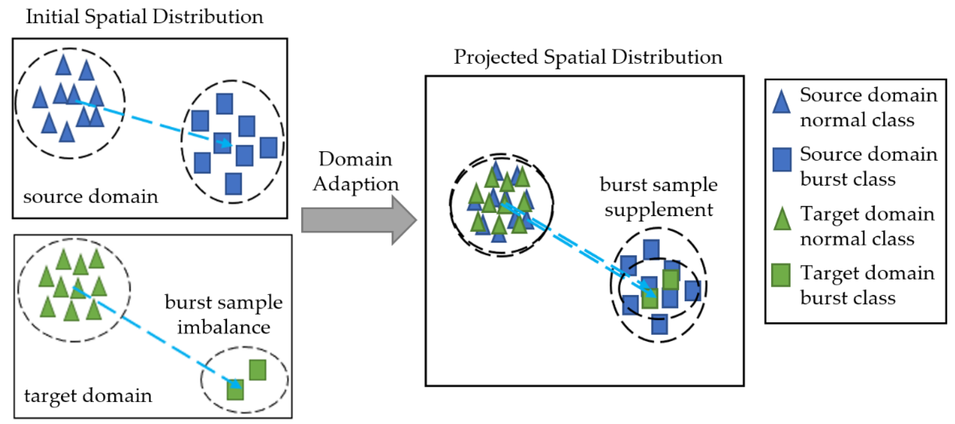
We proposed a machine learning model based on the transfer learning paradigm to solve the data imbalance problem in pipeline-burst detection. This model employs an independent virtual water supply network to generate various types of samples based on the hydraulic formulas, and takes the generated data as the source domain. Then, we employed the domain adaption method to transfer source domain data into the target domain containing practical imbalanced monitoring data. In this way, the incomplete and imbalanced data of the existing water supply network are supplemented. Moreover, the identification and location of pipeline-burst events were obtained based on the supplementary data. The goal of our proposed method is to obtain supplementary data from a hydraulic-model-based virtual pipeline network to an actual pipeline network at a meager cost. Previous hydraulic-model-based methods have two phases: virtual network calibration and actual data generation. The first phase focused on establishing a hydraulic-model-based virtual network that is highly similar to the actual one, requiring a long time to collect actual data for hydraulic-model calibration and considerable expenditure to construct a specific virtual network with topology constraints from the real network. Our proposed method combines these two phases and uses the data from an arbitrary virtual network for data generation, which avoids complex hydraulic-model calibration. The support behind our method is the common-sense idea that a pipeline bursting in any pipeline networks will cause the same trend of pressure and flow changes in the pipelines near the bursting point. That is, common patterns are hidden in datasets from totally different pipeline networks. Thus, we attempt to build a relation between data from very different pipeline topologies containing a common pattern. The mathematical expression of this relation can easily be achieved by the domain adaptation method, a subtype of transfer learning. In other words, costly network reformulation and hydraulic-model calibration can be replaced with a transfer learning model that maps data from a non-constrained network to an actual one. As a result, the data generation for an actual pipeline network is more convenient and cost-saving.

The effect of the proposed method is shown in Figure 1, and its main contributions are as follows:

➀

The transfer learning paradigm is adopted for the first time to transfer the hydraulic model knowledge to an actual water supply network with a low cost.

➁

A specific domain adaptation model is proposed to solve the data imbalance problem in actual pipeline-burst detection.

➂

A closed form solution is deduced for the proposed model.

➃

A three-point-positioning method is presented for pipeline-burst location.

Figure 1. Illustration of proposed method effect.

Figure 1. Illustration of proposed method effect.

The rest of this paper is organized as follows. The Section 2 describes our model and solution, including the relevant applications and theoretical background. Section 3 describes the data sources and forms obtained from virtual and actual water supply networks. The Section 4 represents the experimental settings. Section 5 describes the experimental results and a relevant discussion. Finally, the summary is provided in Section 6.

2. Method

2.1. Motivation

The scarceness of pipeline anomaly in modern water supply networks causes rare pipeline-burst samples but rich normal data. A model trained on these samples and data would learn a distorted classification hyperplane [35,36].

Collecting rare-category samples by creating manufactured burst accidents to enrich the imbalanced dataset in a working pipeline network is impractical. Moreover, generating minor-category samples with mathematical models based on the collected data is inappropriate because we cannot ensure the existing rare-category data contain comprehensive information on all possible pipeline-burst events [30]. Thus, we generated sufficient pipeline-burst events and associated data from the theoretical hydraulic models. Our proposed method requires a virtual pipeline network with theoretical hydraulic models to provide pipeline-burst events and samples at various places and conditions. We can establish this water supply network and obtain the expected data with a simulation tool such as EPANET 2.0 (United States Environmental Protection Agency, Washington, DC, USA) and MATLAB R2020a (MathWorks, Natick, MA, USA).

It is impossible to create a virtual pipeline network identical to the actual working one because of the unacceptable time, expenditure and labor force cost. To solve this problem, we used the domain adaptation method [37,38], an approach of the transfer learning paradigm, to convert pipeline-burst data of a virtual network with an arbitrary topology to a specific practical pipeline network. The domain adaptation method treats the pressure data from two different topological networks as two high-dimensional data spaces. Its goal is to find the mapping projection between these two data spaces. Unlike forward modeling (used by the traditional hydraulic model calibration), which considers many factors, including the pressure gauge position difference, the domain adaptation manner estimates the mapping projection based only on the pressure data in two data spaces. Thus, the learned mapping projection naturally reflects the effectiveness caused by the all the realistic factors of model calibration. We regard the virtual-network-generated data and actual imbalanced data as the source and target domains, respectively. The domain adaptation model aims to learn a mapping function from the source domain to the target domain. As a result, the rare category of the target domain can be supplemented by the customized source domain data through the obtained mapping function.

2.2. Proposed Method

2.2.1. Maximum Mean Difference

The maximum mean difference is an important measure in the domain adaptation [39,40]. It is often applied to evaluate the distribution difference between two datasets in the domain alignment process. $X_S=[x_s^1,x_s^2,\cdots ,x_s^{N_s}]\in R^{D\times N_s}$ and $X_T=[x_t^1,x_t^2,\cdots ,x_t^{N_t}]\in R^{D\times N_t}$ are assumed to be the source domain and the target domain data respectively. D is the dimension of data samples; $N_S$ and $N_T$ are the numbers of the source domain and target domain samples, respectively. MMD computes the difference between two data domains as follows:

$$\mathrm{MMD}\left(X_S,X_T\right)={‖\frac{1}{N_s}{\displaystyle \sum _{i=1}^{N_s}\Phi \left(x_s^i\right)}-\frac{1}{N_t}{\displaystyle \sum _{j=1}^{N_t}\Phi \left(x_t^j\right)}‖}_H^2$$

(1)

where $\Phi \left(\cdot \right)$ represents the mapping function in Hilbert space $H$; $X_S$ and $X_T$ satisfy the edge distribution $P\left(\Phi \left(X_S\right)\right)=P\left(\Phi \left(X_T\right)\right)$. Similar projected data distributions of different domains would be achieved by minimizing Equation (1).

We extended some notations from the basic MMD formula in this study because multiple monitoring water pressure gauges’ value are achieved at many moments instead of a single one; additionally, the dimensions between two domains are generally different. Thus, $X_S=[x_s^1,x_s^2,\dots ,x_s^{N_S}]\in R^{D_S\times N_S}$ and $X_T=[x_t^1,x_t^2,\dots ,x_t^{N_T}]\in R^{D_T\times N_T}$ are used to denote the source and target domain data, respectively, where $D_S$ and $D_T$ are the sample dimensions of these two domains. $N_S=N_S^1+N_S^2$; $N_S^1$ and $N_S^2$ represent the normal and pipeline-burst sample numbers in the source domain, respectively. $N_T=N_T^1+N_T^2$; $N_T^1$ and $N_T^2$ represent the normal and pipeline-burst sample numbers in the target domain, respectively.

2.2.2. Model Formulation

We aimed to find a projection matrix $P\in R^{D_S\times D_T}$ to transfer the samples from the source domain to the target domain. The projection matrix P should simultaneously satisfy the folowing: (1) the mapping source domain samples are aligned with the same kind of target domain sample; (2) the direction of sample movements (pressure-vector variations) should be identical between normal and pipeline-burst classes.

We first set the mapping function in the MMD definition as a linear projection matrix P for lightweight computation. Then, a loss function to align normal samples in different domains can be established as follows:

$$\underset{P}{\min }{L}_1=\underset{P}{\min }{‖P^{\mathrm{T}}{\overline{x}}_s^1-{\overline{x}}_t^1‖}_2^2$$

(2)

where ${\overline{x}}_s^1$ and ${\overline{x}}_t^1$ represent the mean vectors of normal samples in the source and target domains, respectively. Moreover, we use ${\overline{x}}_s^2$ and ${\overline{x}}_t^2$ to represent the mean vectors of pipeline-burst samples in the source and target domains, respectively. A loss function model to align pipeline-burst samples in different domains can be formed as follows:

$$\underset{P}{\min }{L}_2=\underset{P}{\min }{‖P^{\mathrm{T}}{\overline{x}}_s^2-{\overline{x}}_t^2‖}_2^2$$

(3)

In addition, we intend to create relative pressure-vector variations in both the projected source and target domains. Accordingly, we designed a loss function to align the data distribution patterns, as follows:

$$\underset{P}{\min }{L}_3={‖P^{\mathrm{T}}\Delta {\overline{x}}_s-\Delta {\overline{x}}_t‖}_2^2$$

(4)

where $\Delta {\overline{x}}_s=\left({\overline{x}}_s^1-{\overline{x}}_s^2\right)/{\left|{\overline{x}}_s^1-{\overline{x}}_s^2\right|}_2$ and $\Delta {\overline{x}}_t=\left({\overline{x}}_t^1-{\overline{x}}_t^2\right)/{\left|{\overline{x}}_t^1-{\overline{x}}_t^2\right|}_2$ are the standardized distribution variations between normal and pipeline-burst categories in the source and target domains, respectively.

By combining Formulas (2)–(4), the general domain adaptation model can be obtained as follows:

$$\begin{array}{ll}\underset{P}{\min }L& ={‖P^{\mathrm{T}}{\overline{x}}_s^1-{\overline{x}}_t^1‖}_2^2+\alpha {‖P^{\mathrm{T}}{\overline{x}}_s^2-{\overline{x}}_t^2‖}_2^2+\beta {‖P^{\mathrm{T}}\Delta {\overline{x}}_s-\Delta {\overline{x}}_t‖}_2^2\\ & s.t. P^{\mathrm{T}}P=I\end{array}$$

(5)

where α and β are the trade-off parameters; P^TP = I maintains orthogonality projection constraint to the projection matrix P.

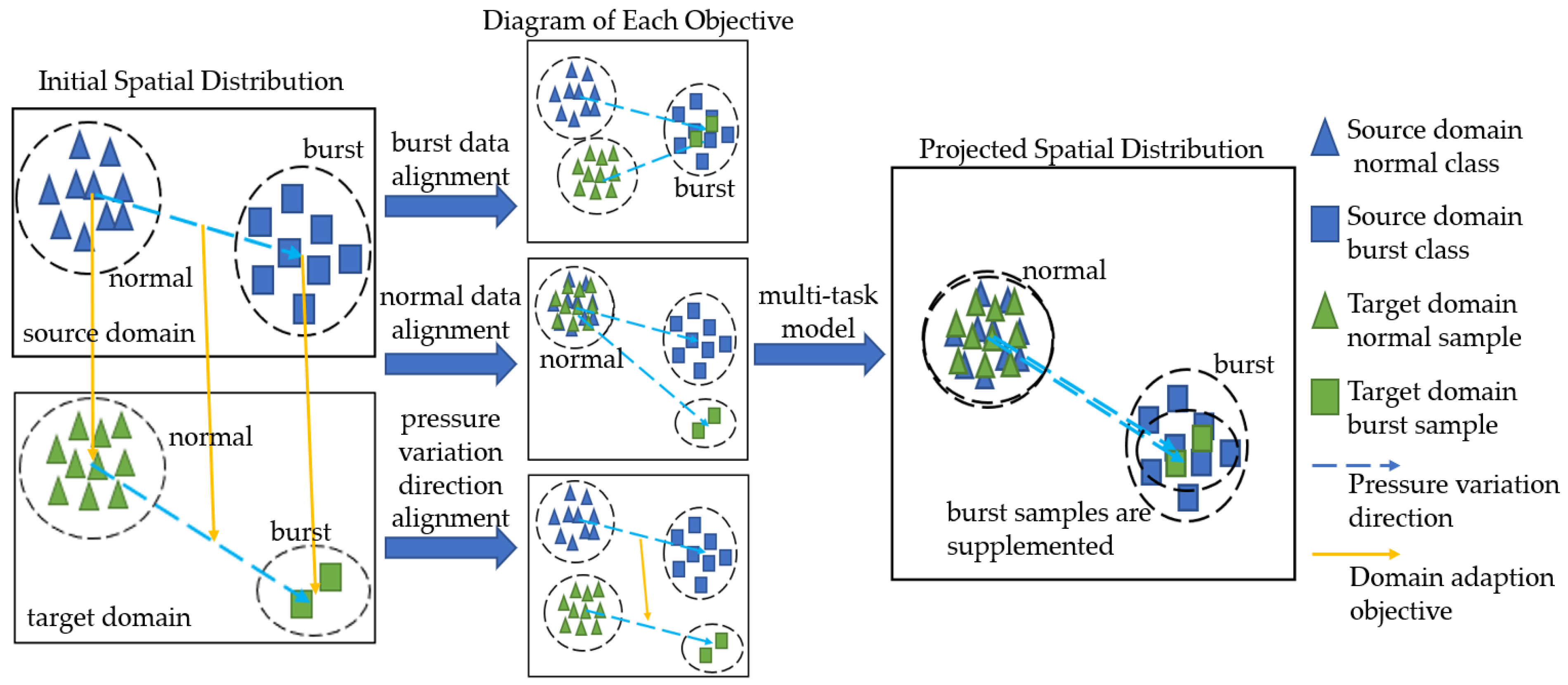
The framework of the proposed model is shown in Figure 2. The burst data alignment, normal data alignment, and pressure variation direction alignment in the figure are oriented from Formulas (2)–(4). The proposed domain adaption model can be obtained by combining these alignments, generating burst samples for the actual network by transfer projection.

2.2.3. Model Solution

We used the Langrange multiplier method to absorb the constraint of Formula (5), as follows:

$$\begin{array}{ll}\underset{P}{\min }L& ={‖P^{\mathrm{T}}{\overline{x}}_s^1-{\overline{x}}_t^1‖}_2^2+\alpha {‖P^{\mathrm{T}}{\overline{x}}_s^2-{\overline{x}}_t^2‖}_2^2\\ & +\beta {‖P^{\mathrm{T}}\Delta {\overline{x}}_s-\Delta {\overline{x}}_t‖}_2^2+\gamma tr(P^{\mathrm{T}}P-I)\\ & =\underset{P}{\min }tr\left({\overline{x}}_s^1{}^{\mathrm{T}}P{P}^{\mathrm{T}}{\overline{x}}_s^1-{\overline{x}}_s^1{}^{\mathrm{T}}P{\overline{x}}_t^1-{\overline{x}}_t^1{}^{\mathrm{T}}{P}^{\mathrm{T}}{\overline{x}}_s^1+{\overline{x}}_t^1{}^{\mathrm{T}}{\overline{x}}_t^1\right)\\ & +\alpha \cdot tr\left({\overline{x}}_s^2{}^{\mathrm{T}}P{P}^{\mathrm{T}}{\overline{x}}_s^2-{\overline{x}}_s^2{}^{\mathrm{T}}P{\overline{x}}_t^2-{\overline{x}}_t^2{}^{\mathrm{T}}{P}^{\mathrm{T}}{\overline{x}}_s^2+{\overline{x}}_t^2{}^{\mathrm{T}}{\overline{x}}_t^2\right)\\ & +\beta \cdot tr\left(\Delta {\overline{x}}_s{}^{\mathrm{T}}P{P}^{\mathrm{T}}\Delta {\overline{x}}_s-\Delta {\overline{x}}_s{}^{\mathrm{T}}P\Delta {\overline{x}}_t-\Delta {\overline{x}}_t{}^{\mathrm{T}}{P}^{\mathrm{T}}\Delta {\overline{x}}_s+\Delta {\overline{x}}_t{}^{\mathrm{T}}\Delta {\overline{x}}_t\right)\\ & +\gamma \cdot tr(P^{\mathrm{T}}P-I)\end{array}$$

(6)

Then, the derivative of Formula (6) can be obtained with respect to P as follows:

$$\begin{array}{ll}\frac{\partial L}{\partial P}& ={\overline{x}}_s^1{\overline{x}}_s^1{}^{\mathrm{T}}P-{\overline{x}}_s^1{\overline{x}}_t^1{}^{\mathrm{T}}+\alpha {\overline{x}}_s^2{\overline{x}}_s^2{}^{\mathrm{T}}P-\alpha {\overline{x}}_s^2{\overline{x}}_t^2{}^{\mathrm{T}}\\ & +\beta \Delta {\overline{x}}_s\Delta {\overline{x}}_s{}^{\mathrm{T}}P-\beta \Delta {\overline{x}}_s\Delta {\overline{x}}_t{}^{\mathrm{T}}+\gamma P\\ & =\left({\overline{x}}_s^1{\overline{x}}_s^1{}^{\mathrm{T}}+\alpha {\overline{x}}_s^2{\overline{x}}_s^2{}^{\mathrm{T}}+\beta \Delta {\overline{x}}_s\Delta {\overline{x}}_s{}^{\mathrm{T}}+\gamma I\right)P\\ & -\left({\overline{x}}_s^1{\overline{x}}_t^1{}^{\mathrm{T}}+\alpha {\overline{x}}_s^2{\overline{x}}_t^2{}^{\mathrm{T}}+\beta \Delta {\overline{x}}_s\Delta {\overline{x}}_t{}^{\mathrm{T}}\right)\end{array}$$

(7)

where γ is the Lagrange multiplier. We define $A={\overline{x}}_s^1{\overline{x}}_s^1{}^{\mathrm{T}}+\alpha {\overline{x}}_s^2{\overline{x}}_s^2{}^{\mathrm{T}}+\beta \Delta {\overline{x}}_s\Delta {\overline{x}}_s{}^{\mathrm{T}}+\gamma I$,$B={\overline{x}}_s^1{\overline{x}}_t^1{}^{\mathrm{T}}+\alpha {\overline{x}}_s^2{\overline{x}}_t^2{}^{\mathrm{T}}+\beta \Delta {\overline{x}}_s\Delta {\overline{x}}_t{}^{\mathrm{T}}$, and let Formula (7) equal zero. Then, the closed-form solution of P is obtained by:

$$P=A^{-1}B$$

(8)

In practice, we can employ a virtual pipeline network to generate customized data as the source domain with balanced category distribution and fill the target domain with samples achieved from an actual operating pipeline network. Then, Formula (8) provides a possible approach to obtaining a projection matrix, transferring the source domain data to the target domain. As a result, the imbalanced data can be balanced by adding transferred minor-category data. We summarize the steps of the proposed method as Algorithm 1.

Algorithm 1: Algorithm steps of proposed method.

Input:

The source domain data matrix XS

The target domain data matrix XT

The trade-off parameter α, β and γ

Output:

Full data matrix X

Procedure:

1: Calculate the mean vectors of normal and pipeline-burst samples ${\overline{x}}_s^1$ and ${\overline{x}}_s^2$ in the source domain XS.

2: Calculate the mean vectors of normal and pipeline-burst samples ${\overline{x}}_t^1$ and ${\overline{x}}_t^2$ in the target domain XT.

3: Calculate the projection matrix P according to Formula (8).

4: Obtain transferred data matrix by PTXS.

5: Form the Full Data matrix X = [PTXS, XT] for classifier training.

3. Dataset Description

We employed 3 virtual and 1 existing actual water supply networks as our study objects. The virtual networks were formulated with different topology structures with EPANET. All the collected data of the virtual networks were nodal water pressures computed by the hydraulic models. We set several diffusion coefficient valves to simulate pipeline-burst events at different locations. Accordingly, we can obtain balanced regular and pipeline-burst samples by category. The actual water supply network data came from a SCADA system of a water supply network in B. District, C. City. All the collected samples were composed of water pressures from either a virtual network’s pipeline nodes or the existing network’s pressure monitoring points. The sample dimensions were consistent with the number of pipeline nodes or pressure monitoring points. In addition, we attached the longitude and latitude information of a pipeline-burst event in the existing network according to the pipeline-burst records of the local water company.

3.1. Actual Water Supply Network

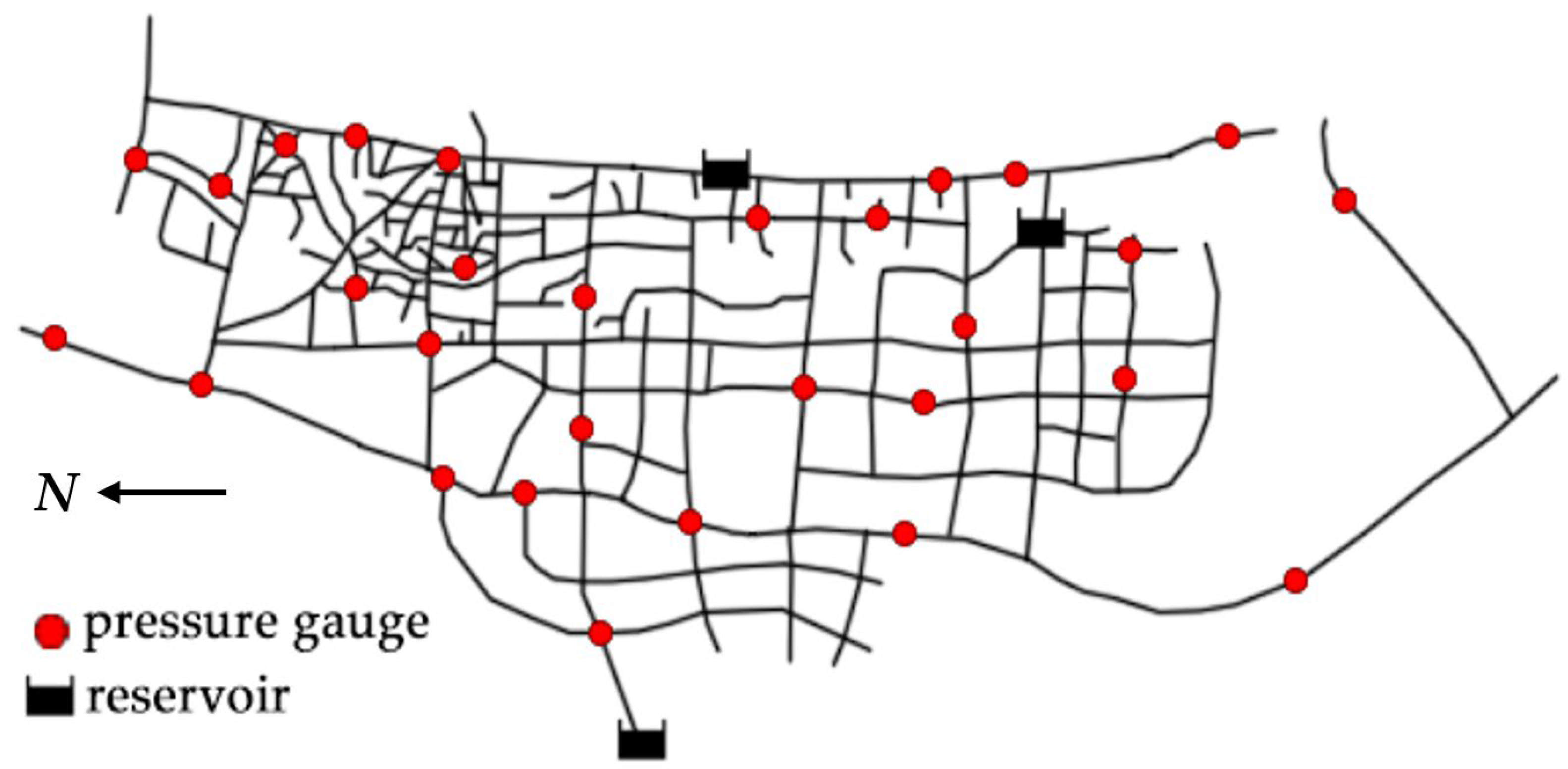
The actual water supply network is generally north–south oriented and covers the central urban area of B. District. The topology structure and detailed information are shown in Figure 3 and

Table 1. Main information of the actual water supply network.

Definition	Amount	Attribute 1		Attribute 2
		Definition	Parameter	Definition	Parameter
reservoir	3	reservoir head	20–100 m
pump	6	pump curve flow	100–600 LPS	pump curve head	20–100 m
pressure gauge	29	pressure	(0–1.2) Mpa
network node	2924	elevation	0–120 ft	flow demand	40–700 L/S
tubulation	10,976	pipe diameter	DN200–DN400	pipe length	50–200 m

, respectively. The actual network is laid according to the direction of street extension, presenting a topology with a grid-like backbone combined with several tree-like terminal structures. There are three waterworks, denoted by reservoir icons in the figure showing the pipeline network. There is a set of water pump units at the waterworks’ outlets, pressurizing the produced tap water and delivering it to the entire network. The network covers nearly 50 square kilometers of the urban area and serves almost 0.2 million people. There are 29 pressure gauges deployed in this network, and the monitoring data are sampled and transmitted via a SCADA system. We collected sampled pressure gauges’ results in 91 days (from 1 September 2020 to 30 November 2020) at the sampling rate of 1 time/hour. In total, 2184 samples with 29 dimensions were obtained, including 106 pipeline-burst and 2078 normal samples. The category imbalance problem was serious in the actual collected data.

3.2. Virtual Water Supply Networks

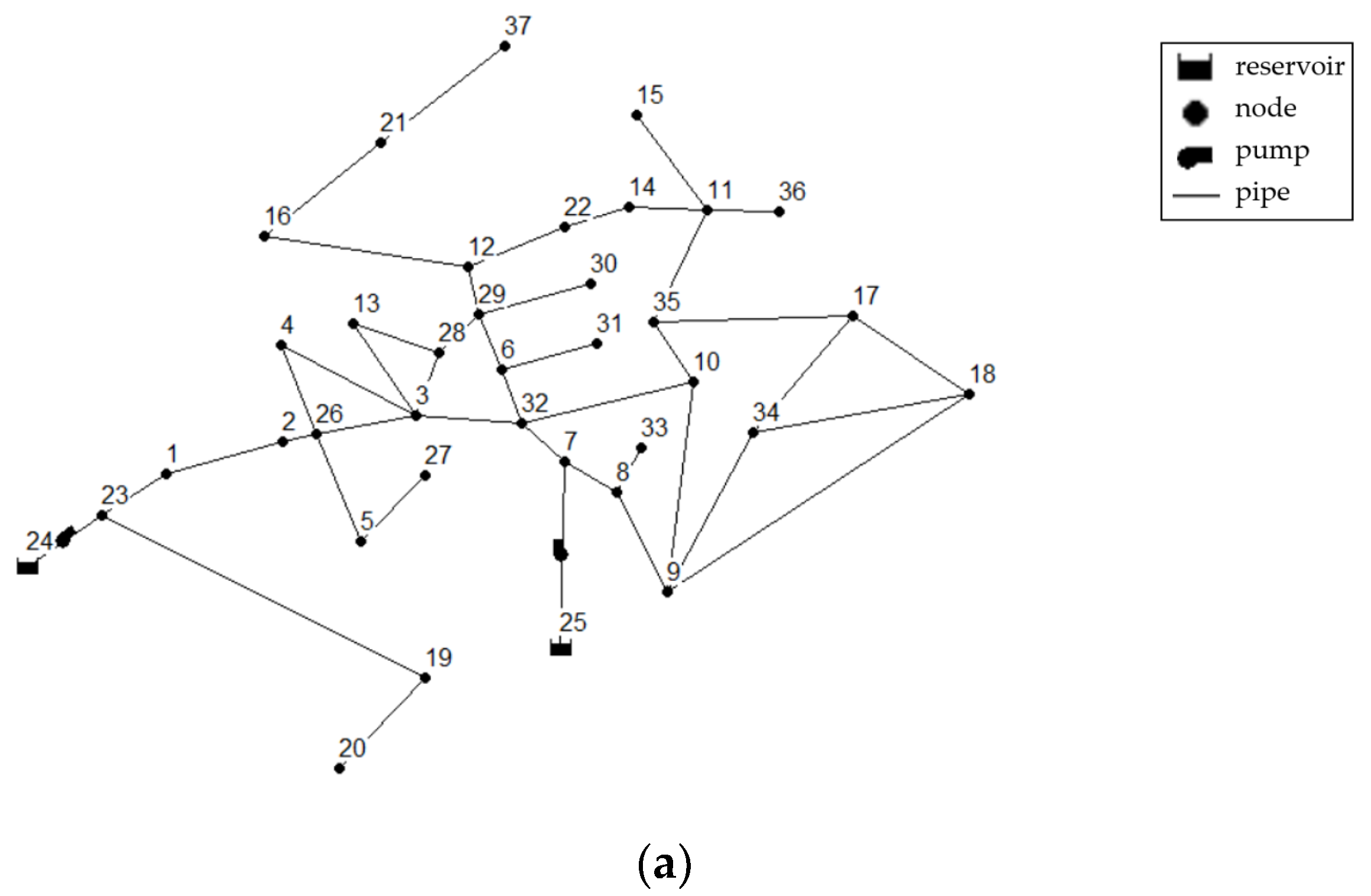
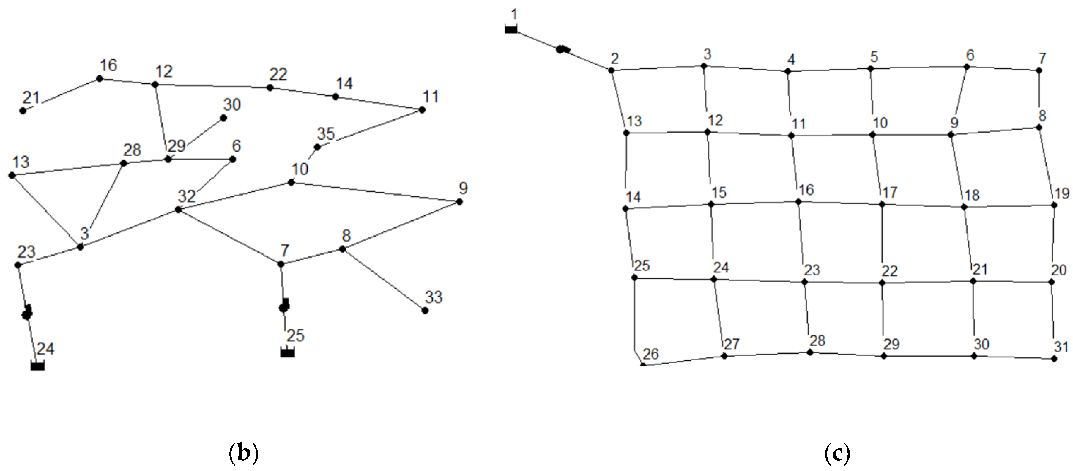
In this study, EPANET was employed to generate sufficient and balanced pipeline-burst samples on three hydraulic-model-based virtual pipeline networks. According to the real water consumption variation of the actual pipeline network in a day, we set a water consumption mode curve for each node in the virtual pipeline networks. A 10% random fluctuation was added to the real water consumption for the water consumption setting of the virtual pipeline networks to enhance sample diversity. We set the diffusion coefficients for pipeline-burst event generation as 8, 10 and 12 at the water consumption setting of the virtual pipeline networks to enhance sample diversity. We also set the topology structure and basic information of the virtual networks A, B and C, which are shown in Figure 4 and

Table 2. Main information of virtual water supply networks.

Pipe Network	Definition	Amount	Attribute 1		Attribute 2
			Definition	Parameter	Definition	Parameter
Virtual Network A	reservoir	2	reservoir head	10–20 m
	pump	2	pump curve flow	400–600 LPS	pump curve head	100–200 m
	pressure gauge	35	pressure	(0–2) Mpa
	network node	37	elevation	5–30 m	flow demand	3–30 LPS
	tubulation	42	pipe diameter	DN100–DN400	pipe length	100–2000 m
Virtual Network B	reservoir	2	reservoir head	10–20 m
	pump	2	pump curve flow	200–300 LPS	pump curve head	100–200 m
	pressure gauge	21	pressure	(1–2) Mpa
	network node	23	elevation	5–30 m	flow demand	3–30 LPS
	tubulation	25	pipe diameter	DN100–DN400	pipe length	100–2000 m
Virtual Network C	reservoir	1	reservoir head	200 m
	pump	1	pump curve flow	700 LPS	pump curve head	300 m
	pressure gauge	30	pressure	(2–5) Mpa
	network node	31	elevation	5–30 m	flow demand	5–15 LPS
	tubulation	23	pipe diameter	DN200–DN300	pipe length	500–800 m

, respectively. The only basis for selecting the three virtual networks was their different topology compared with the actual network. We intentionally caused this situation because our goal was to enrich the actual data from an arbitrary virtual pipeline network instead of a costly calibrated virtual network. We used these three virtual networks according to their different structural complexities. Network A contains the most local topology structures; virtual network B simplifies virtual network A, reducing structural complexity and the collected data dimension. Virtual network C is a standard grid network with a relatively simple regulation. In addition, each virtual network’s data dimension equals its node number, and we set the roughness coefficients of all virtual networks as 100.

We used the actual network’s settings as the virtual ones for pressure data sampling. The dimension of collected pressure data depends on the node numbers of the corresponding network. The locations of pipeline-burst events were set near specific pressure gauges. By simulation, we acquired the normal situation data for 24 h and repeated this 60 times. Then, we assigned an arbitrary burst location with 3 different diffusion coefficients and repeated this 20 times. Thus, we obtained 24 × 60 = 1440 normal and 24 × 3 × 20 = 1440 pipeline-burst single category samples from a virtual network.

Assume that the source and target domains contain sufficient and insufficient pipeline-burst samples, respectively. Thus, we tried to transfer the pipeline-burst data information of the source domain to the target domain to overcome the data imbalance problem. In order to explore the relationship between transfer sample number and anti-imbalance performance, we defined the pipeline-burst sample retention ratio r (0 < r ≤ 1) to indicate data imbalance level:

$$r=N_{collect}/1440$$

(9)

where N_collect is the number of selected samples from 1440 pipeline-burst samples. A smaller r means a greater imbalance level.

4. Experimental Settings

4.1. Scenario Settings

This section verifies the proposed method under two different conditions. Firstly, we used two virtual network datasets for both source and target domains, called a virtual scenario. We can observe the model performance with varied imbalance levels in the target domain. Then, we used a virtual network data and the actual network data as the source and target domains, respectively. This actual scenario was used to validate the imbalance compensation ability of the proposed model in actual conditions.

The virtual scenarios include “A-B” and “A-C”. Scenario “A-B” transfers the data from virtual network A to virtual network B to verify the transfer effect between two pipeline networks with similar topologies. For scenario “A-C”, we mapped the data between two pipeline networks (from virtual network A to virtual network C) to verify the condition of a significant topology difference.

In the actual scenario “A-R”, we chose virtual network A as the source domain network to obtain as much sufficient and various pipeline-burst information as possible, and used the water-pressure-gauge data of the actual network in the target domain.

4.2. Partition Settings

To identify a pipeline-burst event, we adopted a two-stage process. The first stage is to pick up the partition in which a pipeline burst event occurred, and the second stage attempts to locate the longitude and latitude coordinates of the burst point. The proposed method was presented for the first stage, improving the negative impact caused by the data imbalance problem. Moreover, we introduced a simple three-point location method to infer the burst point for the second stage. In this study, we conducted all two stages and the first stage using the actual and virtual scenarios, respectively.

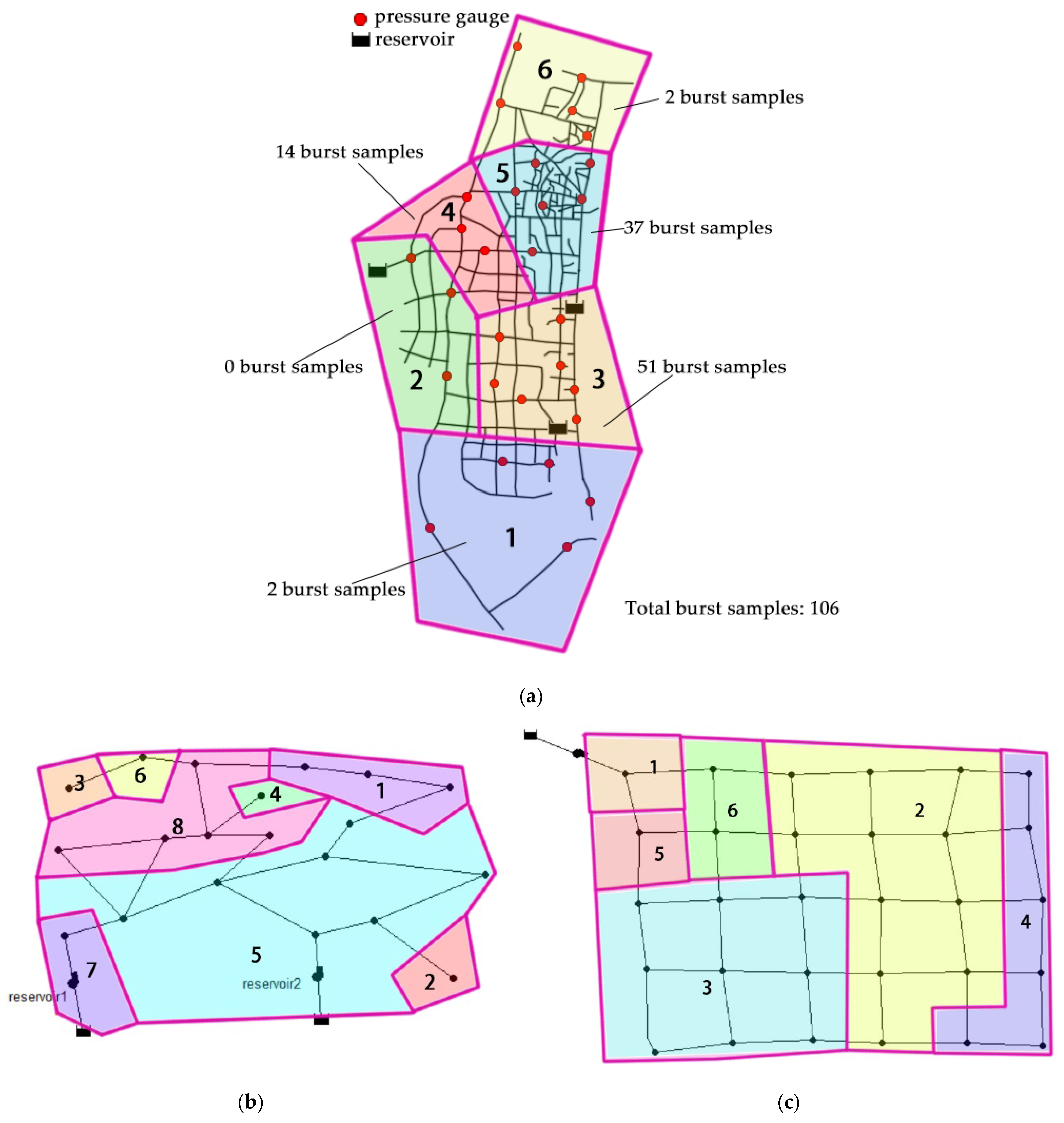
K-means clustering algorithm was applied to divide virtual networks B and C into several partitions according to the Jacobian matrix of pressure variations, which describes the pressure variation difference between monitoring gauges when a burst event occurs [30]. The clustering method aggregates similar monitoring gauges by sensitivity matrices computed from the pressure and flow values [41]. Then, the networks can be assigned to several partitions according to the monitoring data similarity and the gauges’ geographic information. Moreover, we used the prior artificial experience to demarcate the partition borders of the actual pipeline networks. Therefore, as shown in Figure 5a–c, we divided the virtual networks B and C and the actual network into 8, 6 and 6 partitions, respectively. The pipeline-burst event distribution in the actual network was provided in Figure 5a; the major pipeline-burst events occurred in partitions 3, 4 and 5.

4.3. Model Settings

The method proposed in this paper includes three trade-off parameters, α, β and γ, and the optimal trade-off parameter combination was determined to be α = 0.05, β = 0.5 and γ = 0.05 by adjusting the trade-off parameters between [0, 1]. We employed the Kalman filtering method and no-processing approach as reference methods. The Kalman filtering method, a typical outlier detection measure, distinguishes pipeline-burst samples by comparing the predicted and observed values. The no-processing approach uses the imbalanced data directly for the following normal/burst classification [14,15,16].

We used five classifiers, k-nearest neighbors (KNN) [27], radial basis function (RBF)-SVM [22], linear (LIN)-SVM [30], back-propagation neural network (BPNN) [25] and random forest (RF) [23], to achieve the partition-level recognition results for the processed data obtained by the proposed and referenced methods. Considering the overall classification performance, the Monte Carlo method was used to determine the optimal parameters of these classifiers in

Table 3. Classifier parameter settings.

Classifier	Main Parameter Setting
KNN	Neighbors k = 7
RBF-SVM	Standard deviation σ = 10 Penalty coefficient C = 1
LIN-SVM	Penalty coefficient C = 0.5
BPNN	First hide layer = 20 Second hide layer = 15
RF	Tree number = 20

. Specifically, for the Kalman filtering method, pipeline-burst events were classified according to the variation between each pressure gauge’s predicted and observed pressure.

4.4. Hardware Configuration

All the proposed and referenced methods were implemented on a desktop. The hardware configuration of the adopted desktop is as follows:

• CPU: Intel(R) Core(TM) i7-9750H
• Memory: 16.0 GB
• Hard disk: 256 GB SSD + 1 TB HDD

5. Results and Discussion

5.1. Results on Partition-Level Identification

We adopted five-fold cross-validation for the abstract training and testing data for two virtual scenarios, “A-B” and “A-C”. Then, we obtained experimental results for the classifiers under different r values. Accordingly, the average partition-level accuracies of pipeline-burst identification are recorded in

Table 4. Partition-level identification accuracy of virtual scenario “A-B” (%).

Method	Classifier	Burst Sample Retention Degree r
		0.001	0.005	0.01	0.05	0.1	0.3	0.5	1	Average
Proposed method	KNN	57.13	60.47	69.22	82	93.12	99.56	99.87	100	82.67
	RBF-SVM	40.4	63.56	64.41	72.29	74.15	76.11	76.46	77	68.05
	LIN-SVM	51.97	86.77	97.48	99.63	99.87	100	100	100	91.97
	BPNN	40.14	46.35	56.18	83.08	94.97	99.98	100	100	77.59
	RF	48.69	52.77	61.43	86.1	93.72	99.21	99.56	99.83	80.16
No-processing approach	KNN	0	9.32	23.74	53.92	81.62	97.95	99.87	100	58.3
	RBF-SVM	10.94	12.37	15.24	26.93	45.26	60.57	66.53	68.45	38.29
	LIN-SVM	11.07	14.95	20.94	68.86	97.19	100	100	100	64.13
	BPNN	9.3	20.68	28.86	68.66	92.88	99.88	100	100	65.03
	RF	11.4	27.52	40.27	76.75	89.68	98.35	99.25	99.67	67.86
Kalman filtering method	None	48.65	54.51	54.77	54.88	54.92	54.75	54.83	54.82	54.02

and

Table 5. Partition-level identification accuracy of virtual scenario “A-C” (%).

Method	Classifier	Burst Sample Retention Degree r
		0.001	0.005	0.01	0.05	0.1	0.3	0.5	1	Average
Proposed method	KNN	49.46	51.24	64.99	81.71	90.85	98.16	99.67	99.95	79.5
	RBF-SVM	47.54	48.4	52.71	64.73	67.5	68.13	69.34	72.97	61.42
	LIN-SVM	81.09	86.33	91.53	95.04	97.69	99.91	100	100	93.95
	BPNN	42.03	45.67	60.24	90.18	96.43	100	100	100	79.32
	RF	46.13	56.01	65.17	87.4	94.41	98.3	98.81	99.21	80.68
No-processing approach	KNN	0.42	26.82	32.91	70.45	84.03	97.37	99.48	99.95	63.93
	RBF-SVM	8.93	22.44	22.56	34.82	46.45	56.37	59.97	61.56	39.14
	LIN-SVM	7.95	17.61	29.66	86.63	98.32	100	100	100	67.52
	BPNN	19.3	35.05	45.88	84.67	97.1	99.81	100	100	72.73
	RF	22.24	39.67	49.59	84.53	92.77	97.92	98.45	99.18	73.04
Kalman filtering method	None	43.61	47.03	47.09	47.21	47.28	47.34	47.43	47.42	46.80

. The proposed method combined with LIN-SVM has achieved the highest average accuracy, 91.97% and 93.95%, in scenarios “A-B” and “A-C”, respectively. In Table 4, the proposed method leads the no-processing approach by 24.34%, 29.76%, 27.84%, 12.56%, and 12.30% on KNN, RBF-SVM, LIN-SVM, BPNN, and RF, respectively. Similarly, the same trend appeared in Table 5: the proposed method obtains 15.57%, 21.49%, 26.43%, 6.59%, and 7.64% higher average accuracies than the referenced method on KNN, RBF-SVM, LIN-SVM, BPNN, and RF, respectively. The Kalman filter method remains at a low level of average accuracy (54.02% and 46.8% in “A-B” and “A-C”), losing helpful information during its filtering process. We infer that the imbalanced data caused the low performance of both the no-processing and the Kalman filter method. The proposed method maintained its accuracy at a higher level, depending on the minority-class data generated by domain adaptation.

We discover that the partition-level accuracy of each classifier gradually decreases with a reduced retention ratio r in two virtual scenarios, especially when r ≤ 0.1. Class imbalance and incompleteness significantly impacted the classifier’s performance. However, the classification performance did not degrade if r was closed to 1. In terms of classifiers, the partition-level accuracy of a classifier would significantly increase when the proposed method was introduced, especially for the class imbalance situation. The topological complexity of the pipeline network rarely affects the knowledge transfer performance of the proposed method and the accuracy trends have been shown in both Table 5 and

Table 6. Partition-level identification accuracy of actual scenario (%).

Method	Classifier	Burst Sample Retention Degree r
		0.05	0.1	0.3	0.5	1	Average
Proposed method	KNN	64.79	81.46	90.88	95.84	96.64	85.92
	RBF-SVM	72.12	90.66	97.62	98.97	100	91.87
	LIN-SVM	57.49	86.25	95.27	97	99.56	87.11
	BPNN	93.77	94.89	96.3	99.07	98.26	96.46
	RF	22.04	30.37	51.95	70.18	79.63	50.83
No-processing approach	KNN	0	0	7.83	26.8	66.39	20.2
	RBF-SVM	12.34	23.3	53.68	70.99	85.17	49.1
	LIN-SVM	12.34	23.3	23.3	70.99	85.17	43.02
	BPNN	29.01	45.49	80.94	88.86	95.3	67.92
	RF	2.21	5.8	27.81	42.82	70.35	29.8
Kalman filtering method	None	23.58	33.4	55	35.09	36.79	32.77

. Although similar pipeline topologies behind the source and target domain data can improve the average accuracy by 7.77%, 8.27%, 1.41%, 5.97%, and 4.66% on different classifiers, generating data from an arbitrary topological network still significantly improves the recognition performance of burst events.

The proposed method significantly improved partition-level pipeline burst identification reliability and accuracy by projecting sufficient pipeline-burst samples from the source domain to the target domain in scenarios “A-B” and “A-C”.

We used three-fold cross-validation to select training and testing samples for the actual scenario. We also regulated the retention ratio r from 0 to 1 to simulate different class imbalance levels. Table 6 records the average accuracies in this actual scenario. The accuracy results of the actual scenario were similar to those of the virtual ones in terms of the changing trend. Firstly, the proposed method reached the highest average score, 93.95%, with LIN-SVM. Second, the superiority of the proposed method is comprehensive: the proposed method’s scores were 24.34%, 29.76%, 27.84%, 12.56%, and 12.30% higher than the no-processing methods on KNN, RBF-SVM, LIN-SVM, BPNN, and RF, respectively. Thirdly, the proposed method based on the domain adaptation paradigm performed well when many pipeline-burst samples were absent, especially r < 0.1. Compared with the no-processing approach, the proposed model dramatically improves the identification performance of each classifier, even when r is at a relatively high level. These excellent identification results proved that the proposed model was adaptable and robust for actual usage.

5.2. Sensitivity Analysis

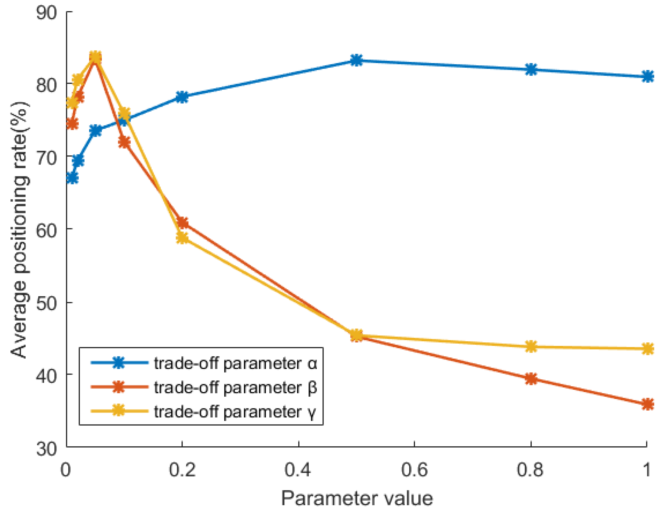
We chose the actual scenario “A-R” as a representation to analyze the parameter sensitivity. We gained partition-level accuracy with different classifiers and retention ratios r = [0.05, 0.1, 0.3, 0.5, 1]. Then, we observed the partition-level accuracy movements along with the trade-off parameter variations. Specifically, we found the optimal trade-off parameter group α = 0.05, β = 0.5, and γ = 0.05 by parameter traversal in [0.01, 1]. We drew the variation curve of each trade-off parameter in Figure 6 by holding the other two trade-off parameters at their optimal values.

As shown in Figure 6, when α is [0.3, 1], the proposed method obtains a high accuracy and low fluctuation curve. This shows that the domain alignment of pipeline-burst data is crucial for obtaining an excellent anti-imbalance performance. A proper β in the range [0.01, 0.1] can maintain the partition identification over 75%, which indicates that the relative position information of pipeline-burst and normal samples can improve the domain adaptation effect. However, if β is too high, the classification accuracy will decline because it weakens the influence of other model terms. Parameter γ is a trade-off parameter of the two-norm regularization term, controlling the approximation and generalization degree of the project matrix. The performance curve of γ shows the same trend as β’s; the best point occurs during the interval [0.01, 0.1]. The performance of the proposed model generally fluctuated with variations in trade-off parameters. Suitable trade-off parameter settings can help to improve performance in actual applications.

5.3. Time Efficiency

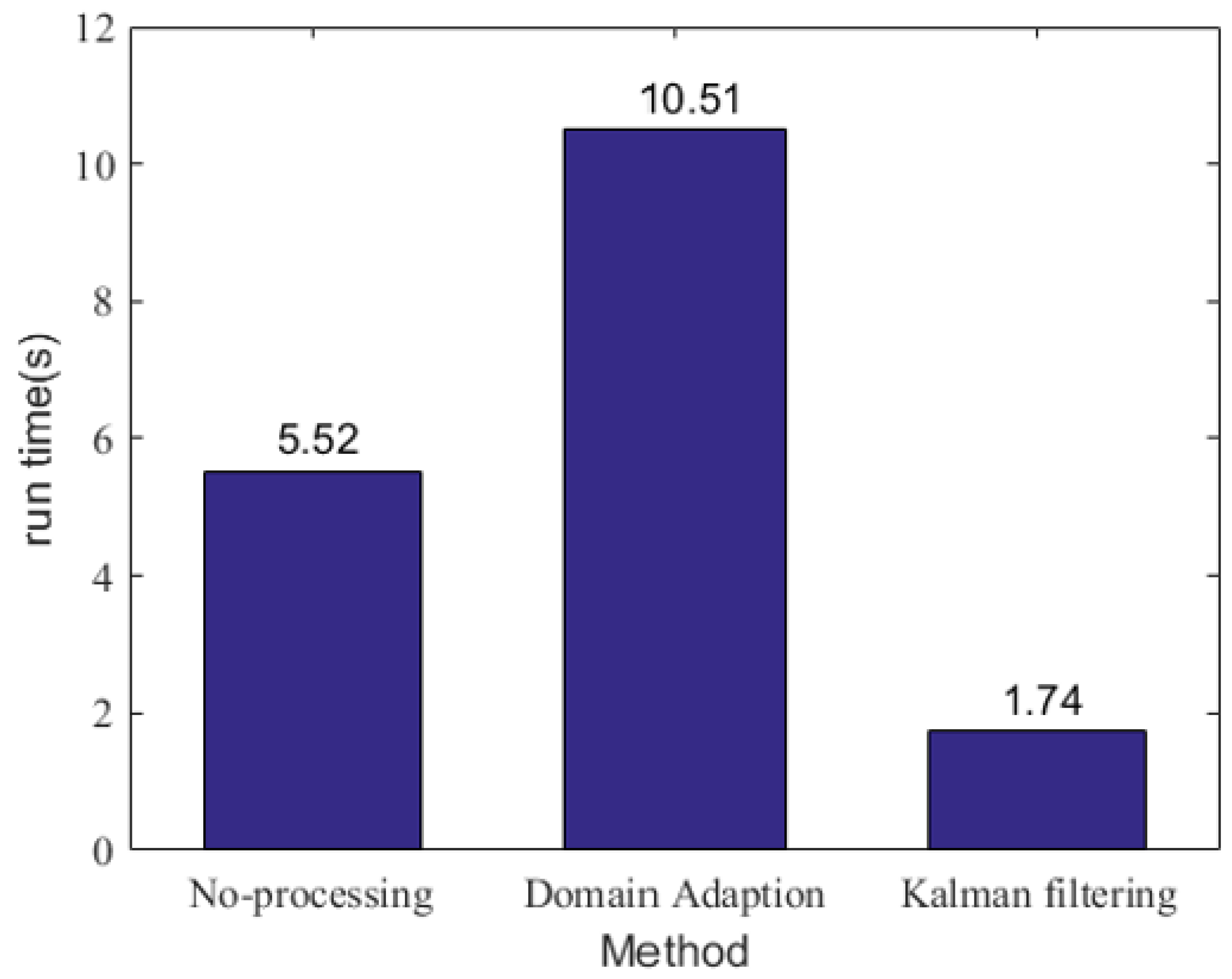
In this subsection, we collected the proposed method’s execution time in the actual scenario compared with the other two referenced methods. Figure 7 represents the time cost of the proposed and reference methods. The time expenditure rank of these three methods is as follows: Kalman filtering method < no-processing approach < the proposed method. The reasons behind this rank are as follows: our proposed method adds a sample generation process to the other two techniques. For the proposed method, obtaining the projection matrix, transferring the pipeline-burst samples from the source domain to the target domain and classifier training required time than the referenced methods. Although the no-processing approach can use data directly without any preprocessing, the following classifiers require a training process for the sampled imbalanced data. The Kalman filtering method takes the least time because of the threshold-based outlier detection mechanism. As a result, the proposed method’s overall time cost is the highest, but acceptable in a water supply network. The distinct anti-imbalance ability of the proposed method is sufficient to make up for the prolonged time expenditure.

5.4. Coordinate Location

In this subsection, we further discuss the pipeline-burst events coordinates of the actual scenario based on the partition-level identification results. We utilized the three-point-positioning principle once used in mobile communication [42,43] to locate a pipleline-burst event according to the longitude and latitude coordinates of the three largest-pressure-fluctuation pressure gauges. Let these three pressure gauges’ longitude and latitude coordinates be two-dimensional vectors x₁, x₂, and x₃. The coordinates of the bust point x can be solved according to the model as follows:

$$\underset{x}{\min }{a}_1{‖x-x_1‖}_2^2+a_2{‖x-x_2‖}_2^2+a_3{‖x-x_3‖}_2^2$$

(10)

where $a_1$, $a_2$, and $a_3$ are the corresponding weight coefficients. Formula (10) is based on the assumption that the burst point will affect the readings of its surrounding pressure gauges, and the closer the pressure gauge is, the greater the impact will be. Therefore, we defined ∆p₁, ∆p₂, and ∆p₃ to represent the relative pressure fluctuations in the first, second and third largest pressure gauges, respectively. Accordingly, $a_1$, $a_2$, and $a_3$ can be calculated by:

$$\begin{array}{l}\left\{\begin{array}{l}{a}_1=\left|\Delta p_1\right|/\left(\left|\Delta p_1\right|+\left|\Delta p_2\right|+\left|\Delta p_3\right|\right)\\ a_2=\left|\Delta p_2\right|/\left(\left|\Delta p_1\right|+\left|\Delta p_2\right|+\left|\Delta p_3\right|\right)\\ a_3=\left|\Delta p_3\right|/\left(\left|\Delta p_1\right|+\left|\Delta p_2\right|+\left|\Delta p_3\right|\right)\end{array}\right.\\ \hspace{0.33em}s.t.\hspace{0.33em}{a}_1+a_2+a_3=1\end{array}$$

(11)

We can achieve x by combining Formulas (10) and (11) as a constrained convex quadratic programming problem.

Table 7. Coordinate location error of pipeline-burst events in the actual network (km).

Classifier	Burst Sample Retention Degree r
	0.05	0.1	0.3	0.5	1
KNN	0.72	0.87	0.77	0.73	0.77
RBF-SVM	0.65	0.94	0.76	0.76	0.76
LIN-SVM	0.70	0.87	0.76	0.77	0.75
ANN	0.86	0.88	0.73	0.85	0.74
RF	0.84	0.57	0.66	0.65	0.63

shows the mean errors of the pipeline-burst point locations in the actual scenario. Through experience, we discovered that the average location error is between 0.57 km and 0.94 km. The results show that the proposed method can support the accurate pipeline-burst location. Using this method, the pipeline-burst location in the actual water supply network reaches the km level, and the error fluctuation between different classifiers is lower than 0.5 km.

6. Conclusions

This paper proposes a domain adaptation method to solve the class imbalance problem in the pipeline-burst detection of a real water supply network. This method establishes a knowledge transfer paradigm to project virtual pipeline-burst samples based on hydraulic models to an existing water supply network. The transferred knowledge can supplement the minority/burst samples in the real world, dealing with the data imbalance problem. Experimental results have proved that our proposed method gains excellent detection ability, especially when the cases of burst samples are extremely deficient. Moreover, we further demonstrated the feasibility of our proposed approach under actual conditions through parameter sensitivity, time efficiency and coordinate location analysis.

In the future, we will continue to enrich the pipe network dataset, study the class-imbalance compensation method in a multi-point burst scene, and improve the mathematical model to avoid the negative transfer effect caused by any disturbing data.

References

- Li, J.; Wu, Y. A Model-Based Bayesian Framework for Pipeline Leakage Enumeration and Location Estimation. Water Resour. Manag. 2021, 35, 4381–4397. [Google Scholar] [CrossRef]
- Wu, Y.; Liu, S. A Review of Data-driven Approaches for Burst Detection in Water Distribution Systems. Urban Water J. 2017, 14, 972–983. [Google Scholar] [CrossRef]
- Romano, M.; Kapelan, Z. Automated Detection of Pipe Bursts and Other Events in Water Distribution Systems. J. Water Resour. Plan. Manag. 2014, 140, 457–467. Available online: https://www.researchgate.net/publication/273369337 (accessed on 15 December 2022). [CrossRef] [Green Version]
- Borges, A.; Jung, D.; Kim, J.H. Smart WDS Management: Pipe Burst Detection Using Real-time Monitoring Data. In Proceedings of the SmartWorld/SCALCOM/UIC/ATC/CBDCom/IOP/SCI, San Francisco, CA, USA, 4–8 August 2017. [Google Scholar]
- Haghighi, A.; Covas, D.; Ramos, H. Direct Backward Transient Analysis for Leak Detection in Pressurized Pipelines: From Theory to Real Application. J. Water Supply Res. Technol. 2012, 61, 189–200. [Google Scholar] [CrossRef]
- Xie, X.; Hou, D.; Tang, X. Leakage Identification in Water Distribution Networks with Error Tolerance Capability. Water Resour. Manag. 2019, 33, 1233–1247. [Google Scholar] [CrossRef]
- Wu, Y.; Liu, S.; Wu, X. Burst Detection in District Metering Areas Using a Data Driven Clustering Algorithm. Water Res. 2016, 100, 28–37. [Google Scholar] [CrossRef] [PubMed]
- Chan, T.K.; Chin, C.S.; Zhong, X. Review of Current Technologies and Proposed Intelligent Methodologies for Water Distributed Network Leakage Detection. IEEE Access 2018, 6, 78846–78867. [Google Scholar] [CrossRef]
- Cheng, W.; Fang, H.; Xu, G. Using SCADA to Detect and Locate Bursts in a Long-Distance Water Pipeline. Water 2018, 10, 1727. [Google Scholar] [CrossRef] [Green Version]
- Laucelli, D.; Romano, M.; Savi, D. Detecting Anomalies in Water Distribution Networks Using EPR Modelling Paradigm. J. Hydroinform. 2015, 18, 409–427. Available online: http://iwaponline.com/jh/article-pdf/18/3/409/478927/jh0180409.pdf (accessed on 15 December 2022). [CrossRef] [Green Version]
- Abdulshaheed, A.; Mustapha, F.; Ghavamian, A. A Pressure-based Method for Monitoring Leaks in a Pipe Distribution System: A Review. Renew. Sustain. Energy Rev. 2017, 69, 902–911. [Google Scholar] [CrossRef]
- Srirangarajan, S.; Allen, M.; Preis, A. Wavelet-based Burst Event Detection and Localization in Water Distribution Systems. J. Signal Process. Syst. 2013, 72, 1–16. [Google Scholar] [CrossRef] [Green Version]
- Zhou, X.; Tang, Z.; Xu, W. Deep Learning Identifies Accurate Burst Locations in Water Distribution Networks. Water Res. 2019, 166, 115058. [Google Scholar] [CrossRef] [PubMed]
- Okeya, I.; Kapelan, Z.; Hutton, C. Online Burst Detection in a Water Distribution System Using the Kalman Filter and Hydraulic Modelling. Procedia Eng. 2014, 89, 418–427. [Google Scholar] [CrossRef] [Green Version]
- Santos-Ruiz, I.; Bermúdez, J.R.; López-Estrada, F.R. Online Leak Diagnosis in Pipelines Using an EKF-Based and Steady-State Mixed Approach. Control Eng. Pract. 2018, 81, 55–64. [Google Scholar] [CrossRef]
- Ye, G.; Fenner, R.A. Kalman Filtering of Hydraulic Measurements for Burst Detection in Water Distribution Systems. J. Pipeline Syst. Eng. Pract. 2011, 2, 14–22. [Google Scholar] [CrossRef]
- Jung, D.; Kang, D.; Liu, J.; Lansey, K. Improving the Rapidity of Responses to Pipe Burst in Water Distribution Systems: A Comparison of Statistical Process Control Methods. J. Hydroinform. 2015, 17, 307–328. Available online: https://www.researchgate.net/publication/276786519 (accessed on 15 December 2022). [CrossRef]
- Lee, S.J.; Lee, G.; Suh, J.C. Online Burst Detection and Location of Water Distribution Systems and Its Practical Applications. J. Water Resour. Plan. Manag. 2016, 142, 4015033. [Google Scholar] [CrossRef]
- Mounce, S.R.; Boxall, J.B.; Machell, J. Development and Verification of an Online Artificial Intelligence System for Detection of Bursts and Other Abnormal Flows. J. Water Resour. Plan. Manag. 2010, 136, 309–318. Available online: https://www.researchgate.net/publication/221936175 (accessed on 15 December 2022). [CrossRef]
- Shukla, H.; Piratla, K.R. Leakage Detection in Water Pipelines Using Supervised Classification of Acceleration Signals. Autom. Constr. 2020, 117, 103256. [Google Scholar] [CrossRef]
- Soldevila, A.; Fernandez-Canti, R.M.; Blesa, J. Leak localization in water distribution networks using Bayesian classifiers. J. Process Control 2017, 55, 1–9. [Google Scholar] [CrossRef] [Green Version]
- Salam, A.; Tola, M.; Selintung, M. A leakage detection system on the Water Pipe Network through Support Vector Machine method. In Proceedings of the Makassar International Conference on Electrical Engineering and Informatics, Macassar, India, 26–30 November 2014. [Google Scholar]
- Hindy, H.; Brosset, D.; Bayne, E. Improving SIEM for Critical SCADA Water Infrastructures Using Machine Learning. In Computer Security: CyberICPS 2018, 1st ed.; Katsikas, S.K., Cuppens, F., Cuppens, N., Lambrinoudakis, C., Antón, A., Gritzalis, S., Mylopoulos, J., Kalloniatis, C., Eds.; Springer: Cham, Switzerland, 2019; pp. 3–19. [Google Scholar]
- Phan, H.C.; Dhar, A.S. Predicting Pipeline Burst Pressures with Machine Learning Models. Int. J. Press. Vessel. Pip. 2021, 191, 104384. [Google Scholar] [CrossRef]
- Mounce, S.R.; Machell, J. Burst Detection Using Hydraulic Data from Water Cistribution Systems with Artificial Neural Networks. Urban Water J. 2006, 3, 21–31. [Google Scholar] [CrossRef]
- Mounce, S.R.; Mounce, R.B.; Boxall, J.B. Novelty Detection for Time Series Data Analysis in Water Distribution Systems Using Support Vector Machines. J. Hydroinform. 2011, 13, 672–686. [Google Scholar] [CrossRef]
- Levinas, D.; Perelman, G.; Ostfeld, A. Water Leak Localization Using High-Resolution Pressure Sensors. Water 2021, 13, 591. [Google Scholar] [CrossRef]
- Sun, C.; Parellada, B.; Puig, V. Leak Localization in Water Distribution Networks Using Pressure and Data-Driven Classifier Approach. Water 2020, 12, 54. Available online: https://www.researchgate.net/publication/338104420 (accessed on 15 December 2022). [CrossRef] [Green Version]
- Tao, T.; Huang, H.; Li, F. Burst Detection Using an Artificial Immune Network in Water-Distribution Systems. J. Water Resour. Plan. Manag. 2014, 140, 4014027. [Google Scholar] [CrossRef]
- Zhang, Q.; Wu, Z.Y.; Zhao, M. Leakage Zone Identification in Large-Scale Water Distribution Systems Using Multiclass Support Vector Machines. J. Water Resour. Plan. Manag. 2016, 142, 4016042. [Google Scholar] [CrossRef]
- Meier, R.W.; Barkdoll, B.D. Sampling Design for Network Model Calibration Using Genetic Algorithms. J. Water Resour. Plan. Manag. 2000, 126, 245–250. [Google Scholar] [CrossRef]
- Schaetzen, D.; Walters, F. Optimal Sampling Design for Model Calibration Using Shortest Path, Genetic and Entropy Algorithms. Urban Water J. 2000, 2, 141–152. [Google Scholar] [CrossRef]
- Kapelan, Z.; Savic, D.; Walters, G. Optimal Sampling Design Methodologies for Water Distribution Model Calibration. J. Hydraul. Eng. 2005, 131, 190–200. [Google Scholar] [CrossRef]
- Bush, C.A.; Uber, J.G. Sampling Design Methods for Water Distribution Model Calibration. J. Water Resour. Plan. Manag. 1998, 124, 334–344. [Google Scholar] [CrossRef]
- Pan, S.J.; Qiang, Y. A Survey on Transfer Learning. IEEE Trans. Knowl. Data Eng. 2010, 22, 1345–1359. [Google Scholar] [CrossRef]
- Duan, L.; Tsang, I.W.; Xu, D. Domain Transfer Multiple Kernel Learning. IEEE Trans. Pattern Anal. Mach. Intell. 2012, 34, 465–479. [Google Scholar] [CrossRef]
- Liu, F.; Zhang, G.; Lu, J. Heterogeneous domain adaptation: An unsupervised approach. IEEE Trans. Neural Netw. Learn. Syst. 2017, 31, 5588–5602. [Google Scholar] [CrossRef] [Green Version]
- Liu, T.; Chen, Y.; Li, D. Drift Compensation for an Electronic Nose by Adaptive Subspace Learning. IEEE Sens. J. 2019, 20, 337–347. [Google Scholar] [CrossRef]
- Pan, S.J.; Tsang, I.W.; Kwok, J.T. Domain adaptation via transfer component analysis. IEEE Trans. Neural Netw. 2011, 22, 199–210. [Google Scholar] [CrossRef] [Green Version]
- Long, M.; Wang, J.; Ding, G. Transfer Feature Learning with Joint Distribution Adaptation. In Proceedings of the 2013 IEEE International Conference on Computer Vision, Sydney, Australia, 4–6 December 2018. [Google Scholar]
- Morosini, A.; Caruso, O. Identification of Measurement Points for Calibration of Water Distribution Network Models. In Proceedings of the 16th Conference on Water Distribution System Analysis, WDSA 2014, Bari, Italy, 14–17 July 2014. [Google Scholar]
- Shalaby, M.; Shokair, M.; Messiha, N.W. Performance Enhancement of TOA Localized Wireless Sensor Networks. Wirel. Pers. Commun. 2017, 95, 4667–4679. [Google Scholar] [CrossRef]
- Kim, J. Hybrid TOA–DOA techniques for maneuvering underwater target tracking using the sensor nodes on the sea surface. Ocean. Eng. 2021, 242, 110110. [Google Scholar] [CrossRef]
Figure 2.
Model diagram of proposed method.
Figure 3.
Topology of actual water supply network in B. District.
Figure 4.
Topology of virtual water supply networks: (a) virtual network A, (b) virtual network B, (c) virtual network C. The numbers in the figures denote different nodes that generate monitoring data.
Figure 5.
Partition settings of water supply networks: (a) actual network; (b) virtual network B; (c) virtual network C.
Figure 6.
Parameter sensitivity curves of the proposed method.
Figure 7.
Time efficiency of methods.