Groundwater Prospecting Using a Multi-Technique Framework in the Lower Casas Grandes Basin, Chihuahua, México

Abstract

Groundwater is a strategic resource for economic development, social justice, environmental sustainability, and water governance. The lower Casas Grandes River Basin, located in the state of Chihuahua, México, is in a semi-arid region with increasing groundwater demand and regional challenges such as drought and depletion of aquifers. Even though there is official information about the availability of groundwater, a comprehensive aquifer characterization requiring an interdisciplinary investigation using a diverse suite of tools and multiple data sources has yet to be carried out. This study presents a multi-technique framework to evaluate potential sites to drill for groundwater resources and reduce the risk of unsuccessful drilling. The main components of the methodology include wellhead leveling correction with a differential global positioning survey to define piezometric levels, principal component analysis using LANDSAT-8 images, application of geospatial tools, geophysics analysis using time domain electromagnetic surveys (TDES) and vertical electric soundings (VES), and structural geohydrology to define aquifer characteristics. The results showed that using the proposed framework steps improved the possibility of identifying subsurface layers with lower resistivity values that could be related to groundwater. Low resistivity values (35 Ohm-m) were found at depths from 50 to 85 m at sites where the regional static water level reached a depth of 245 m, indicating the potential location of a shallow groundwater resource at a site where the intersection of a fracture trace was identified. This procedure can be used in other regions in the world where limited information is available for groundwater exploration, thus reducing the risk of drilling dry wells in complex hydrogeological environments.

1. Introduction

Groundwater (GW) has become one of the most important sources of water around the world, and transboundary aquifer characterization is important for a sustainable approach to binational groundwater governance [1]. GW is the main water resource in arid and semi-arid zones, representing more than 99% of liquid freshwater availability in the world [2] and approximately 0.75% of all the existing water in the world [3]. However, groundwater is one of the least studied and understood water sources in terms of its nature, formation, movement, quality, recharge, availability, and extension worldwide [4]. Lying between México and the United States, the Chihuahua Desert is one of the largest deserts in the world and is shared between the two nations. GW is used to supply water to cities, industries, and agriculture in the desert plains of the state of Chihuahua and has received significant attention in recent years [5]. However, GW in the state of Chihuahua has been compromised in recent years due to drought, population growth, climate change, and over-concessions, which have impacted aquifers. A decrease in piezometric levels of transboundary aquifers has depleted shallow aquifers (<200 m) [6]. According to the Mexican water agency, Comisión Nacional del Agua (CONAGUA) [7,8], approximately 72% of the water concessions assigned in México correspond to agricultural uses where groundwater inventories in the closed basins of northern México are limited. In recent years, a drop in piezometric levels has been identified in these aquifers, varying from 35 cm to 1.5 m per year over the past 20 years [9]. Within the geographical location of the state of Chihuahua, areas of high population growth, water withdrawals for crop irrigation and providing water for livestock, drought, and increasing temperatures have made the state vulnerable to the overuse of aquifers [10].

The Ascensión aquifer, located in northern Chihuahua, México, was formed in alluvial deposits (Figure 1 and Figure 2) [7]. The approximate direction in which groundwater movement occurs in Chihuahua is towards heavy pumping areas (Figure 1). However, when extending the static water level (SWL) equipotential trends into the study area of interest in this report, fractured conglomerates in the upper parts of the basin promote infiltration from the headwaters of the watershed, which could flow downslope until it intercepts the regional SWL of the Ascensión aquifer (Figure 3). Official publications from the Mexican water authority (CONAGUA) [7] have reported that Ascensión Valley originated from tectonic rifts that filled with deposits of alluvial materials of very heterogeneous granulometry. It is an unconfined aquifer unit with medium to high permeability characteristics. The upper shallow aquifer of alluvial deposits has intermittent recharge from the deeper, underlying regional Janos aquifer [10]. Transmissivity values in the Janos aquifer, according to a study carried out in 1972 by CONAGUA, ranged from 1 to 50 × 10⁻³ m²/s, with an average value of 4 × 10⁻³ m²/s. According to an updated 1979 study, the transmissivity values were less than 5 × 10⁻³ m²/s. In the Ascensión aquifer, which presents similar geological characteristics as the Janos aquifer, the average value of transmissivity was estimated to be 4 × 10⁻³ m²/s. The value of the storage coefficient was estimated to be in the order of 0.03. The average aquifer thickness at the Mexican section of the Basin and Range Province, where the lower Casas Grandes River Basin is located, varies from 300 to 2000 m in depth [10]. The recharge to the Ascensión aquifer comes from the area where the Casas Grandes River and the Salto del Ojo stream are located; however, local recharge occurs from rainwater that infiltrates the mountain front at Sierra del Capulín (study site; Figure 2). Recharge also occurs in the eastern part of the El Fresnal mountain range. The lower parts of the valley also allow recharge to the aquifer through rainwater infiltration and irrigation water returns [7]. According to CONAGUA [7], the natural recharge, considered as the sum of the infiltration of rainwater plus the subterranean flow coming from the mountainous areas that surround the valley and from the southwestern part of the Janos aquifer, has been calculated at 94.2 MCM/year (millions of cubic meter per year). For rainwater recharge, a valley area of 2000 km² was considered, with a precipitation of 289.4 mm and an infiltration coefficient of 0.08, which gave a natural recharge of 48.6 MCM/year. Horizontal recharge by lateral flow was estimated at 45.6 hm³/year. The induced recharge comes from groundwater used for irrigation and a lower proportion comes from water used for domestic and urban public uses. The total amount of induced recharge has been calculated at 38.0 hm³/year by multiplying the volume applied to irrigation (187 MCM/year of groundwater) by an infiltration coefficient of 0.20 and multiplying the volume used in domestic and public urban uses (3.04 MCM/year) by a coefficient of 0.20. The average range of well yields at the Janos aquifer site varies from 10 to 150 L/s [10]. Most of the well infrastructure is designed to pump an average of 64 L/s and the total extraction of groundwater in the area is approximately 241.2 hm³/year (20 February 2020) [11]. This is mainly for agriculture and to a much lesser extent for domestic, urban, and industrial uses.

Tributaries on the hills of the Sierra del Capulin as well as the arroyo watercourses at the headwaters of the basin could contribute to the recharge process. Furthermore, the linear fractured conglomerates that were altered by tectonic forces of the regional natural geological formation are assumed to produce local recharge from the headwaters in the watershed. It has been reported that recharge lineaments formed by the arroyos can feed water recharge to the underlying rock formations if these have some degree of fracturing or secondary porosity [12]. The average annual groundwater availability in 1998 for the Ascension aquifer was published by official sources [7]. Equipotentials in this report defined a groundwater flow system moving from the Sierra del Capulín towards Laguna San Juan (Figure 1). Because the information on the elevation of SWL and piezometric measurements were officially obtained in 1998, it was necessary to update the values of this parameter by carrying out a survey of recent equipotentials and updating piezometric levels in the area.

The present study aimed to support prospecting for groundwater using a multi-task approximation to locate potential drilling sites in a basin with semi-arid climatic conditions, complex geological settings, and depletion of groundwater levels. The focus was to locate a well site to provide water for livestock. Given the site’s complex hydrogeological conditions, finding a location for a potential drilling point that could supply a minimum volume for the development of this activity was complicated. The procedure was based on the use of traditional methods, such as the characterization of structural geology, surveys of wells, and fieldwork with global positioning systems real-time kinematics (GPS RTK), and remote sensing through the spectral analysis of satellite images with statistical techniques (e.g., principal component analysis). There are few studies of the aquifers in Chihuahua [7,9,10], and in the case of the study area, information is scarce or lacks the detail required to make the extraction of groundwater more sustainable [9]. The situation is similar throughout the arid north of México, where problems of overuse of groundwater and the absence of data are widespread [13]. Both are crucial issues for the sustainability of water; therefore, characterization of the aquifer combining remote-sensing data, mathematical analysis, and traditional geophysical methods could contribute to the management of groundwater and its governance by water-resource managers. Addressing these issues is necessary for the sustainability of water, particularly in the United States–México binational region and in all of the northern states of México.

This paper applied a multi-technique framework to support well placement efforts in the lower Casas Grandes River Basin (CGRB), thus improving the efficiency of successful drilling for groundwater resources and proving the innovation of our work. Agricultural and livestock production are economically important for agricultural communities in the desert plains of the state of Chihuahua [6,13]. Recurrent droughts in the area have caused an urgent need to find new sources of water, including in the upper region of the Sierra del Capulín [8]. Figure 3 shows a conceptual model of the structural geology and its relationship with the regional aquifer in the study area where several failed drilling attempts have jeopardized the rural development of a local ranch. The absence of water at the headwaters of the watershed made it necessary to implement a pumping system to provide water upstream from a source located in the valley situated to the southwest of the study area. The use of water is primarily for cattle, so a source that produces a large volume of water is not required. The costs involved in pumping water from the well located downstream in the valley to the upper part of the mountain front justified a geohydrological study and geophysical prospecting to identify suitable sites for a supply well for the ranch in order to replace water importation from downstream areas. Many ranchers in the area are struggling to access water to provide to their cattle. Hence, they are willing to risk high investments to solve their water problems. Furthermore, since new pumping technology is available, many of these ranchers are installing solar panel infrastructure to pump groundwater at greater depths. Low-yield wells (1 or 2 L/s) could make a significant difference and provide lifesaving infrastructure for these families. The presented framework is important since it can be applied in other regions to increase the success of well drilling efforts at suitable sites identified through robust hydrogeological investigations [14].

2. Materials and Methods

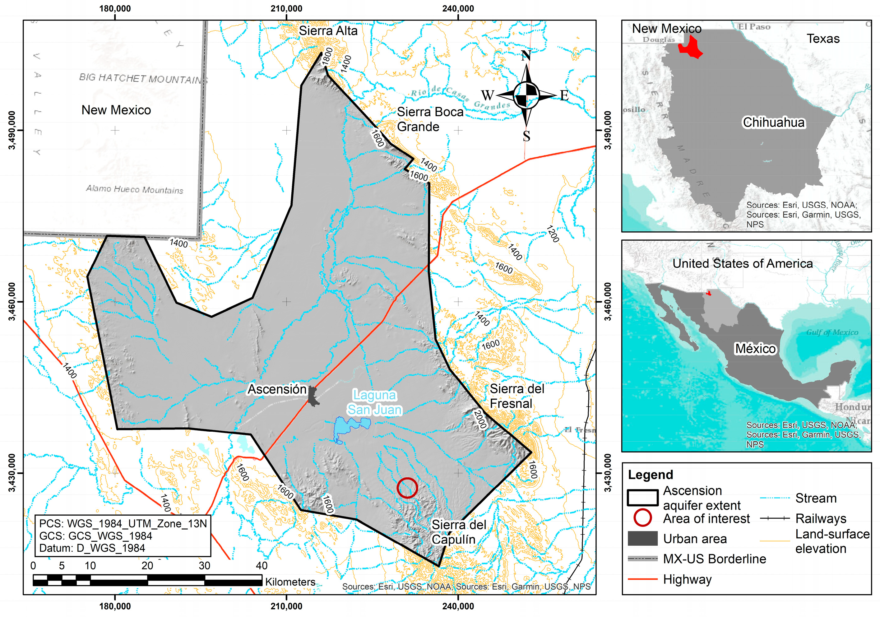
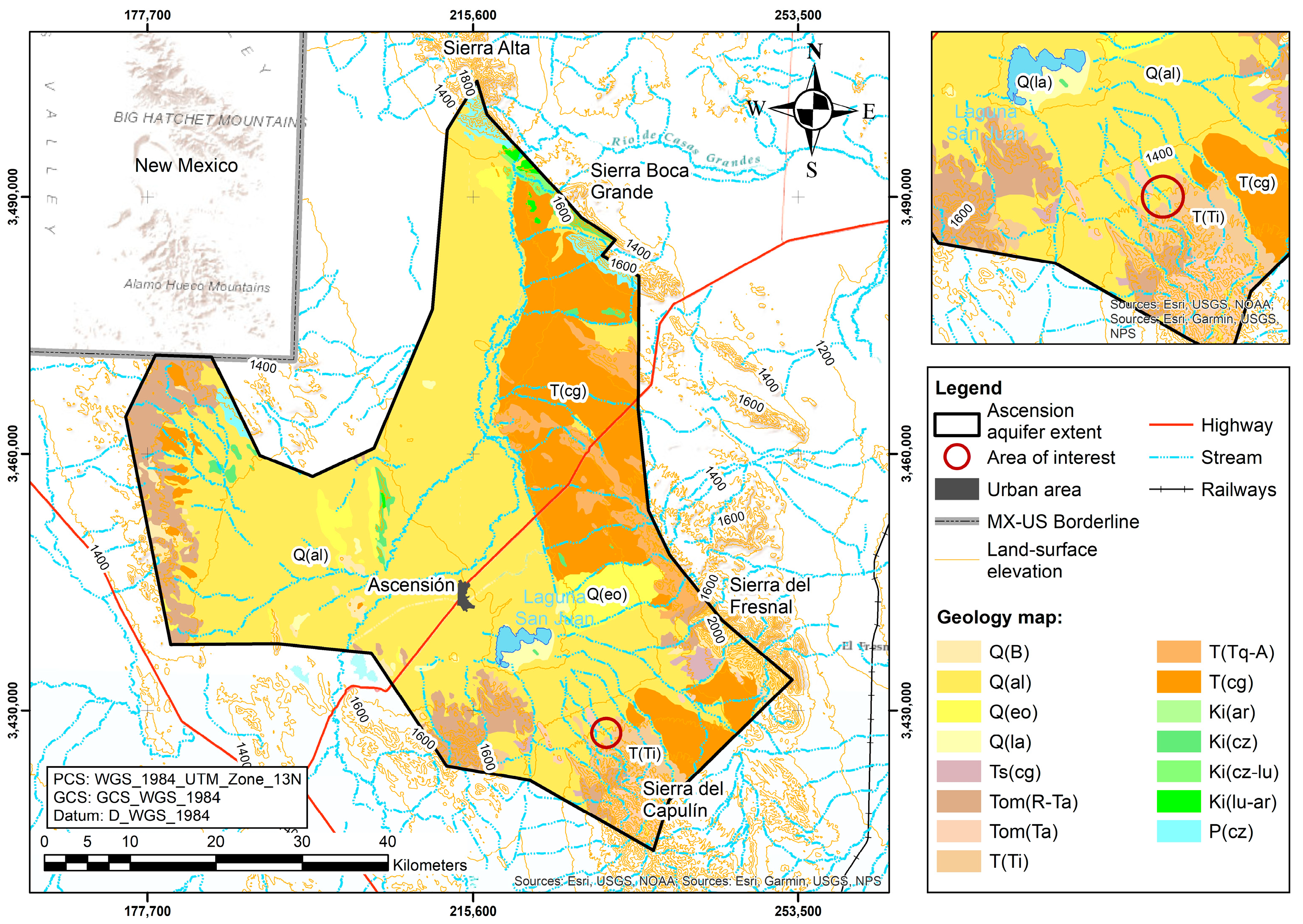
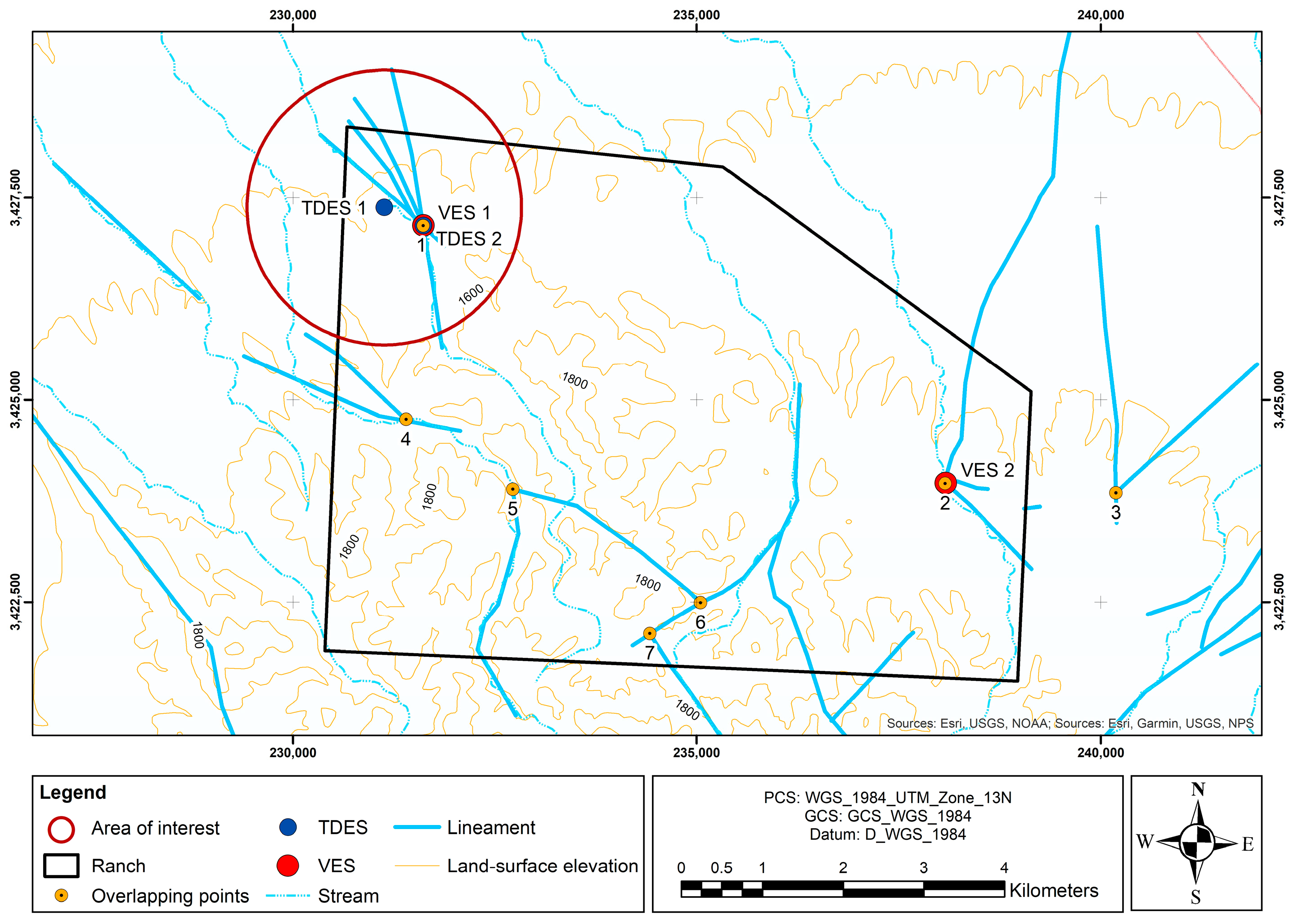
2.1. Study Area

The study area is a local ranch in Ascensión, Chihuahua, México, south of Luna County, New Mexico, United States. The location is approximately 31 km from the town of Ascensión, near Laguna San Juan, which is located to the side of the slopes of Sierra del Capulín (Figure 2). It is a region characterized by agricultural and livestock activity, and the water supply is the local Ascension aquifer [7]. Surface water flows toward the topographic low point at the Laguna San Juan, where runoff gathers during the rainy season and eventually evaporates (Figure 2). In Ascensión, Chihuahua, the summers are warm and partly cloudy, and the winters are short, cold, dry, and mostly clear. During the year, the average monthly temperature ranges from 9 °C in January to 28 °C in June, rarely falling below −4 °C or rising above 40 °C. The minimum daily average temperature is 4 °C in January, and the maximum daily temperature reaches 40 °C in June. The average annual rainfall is approximately 300 mm and the average annual relative humidity is 42% [7].

The direction in which groundwater moves in the study area is represented by arrows, which show the direction of the flow, while the equipotential lines represent the groundwater elevation measured in meters above sea level (masl). The equipotential elevation closest to the area of interest, according to this database, had an elevation of 1300 masl in 1998, and the topographic elevation at the area of interest (red circle in Figure 1) was measured to be approximately 1530 masl.

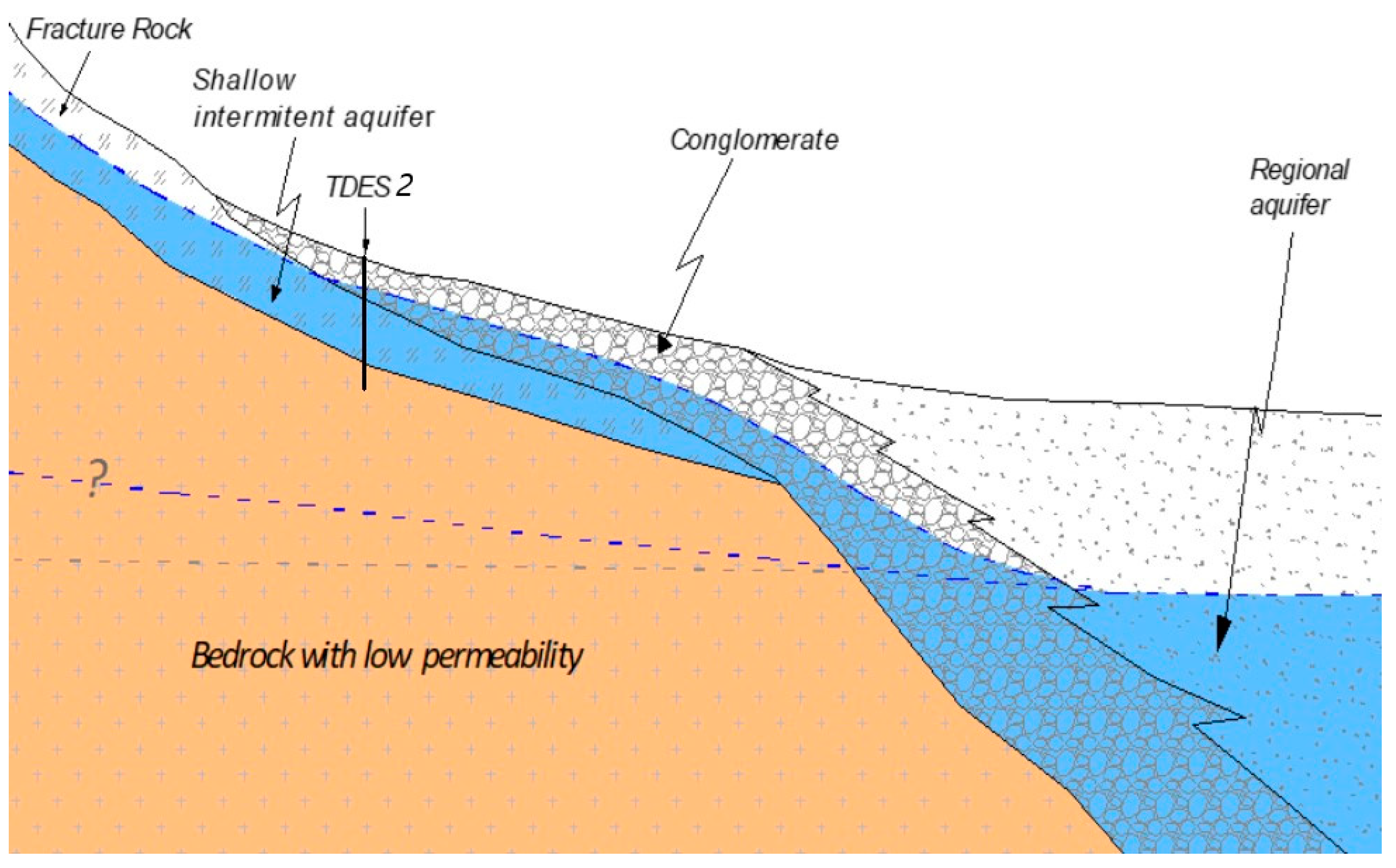
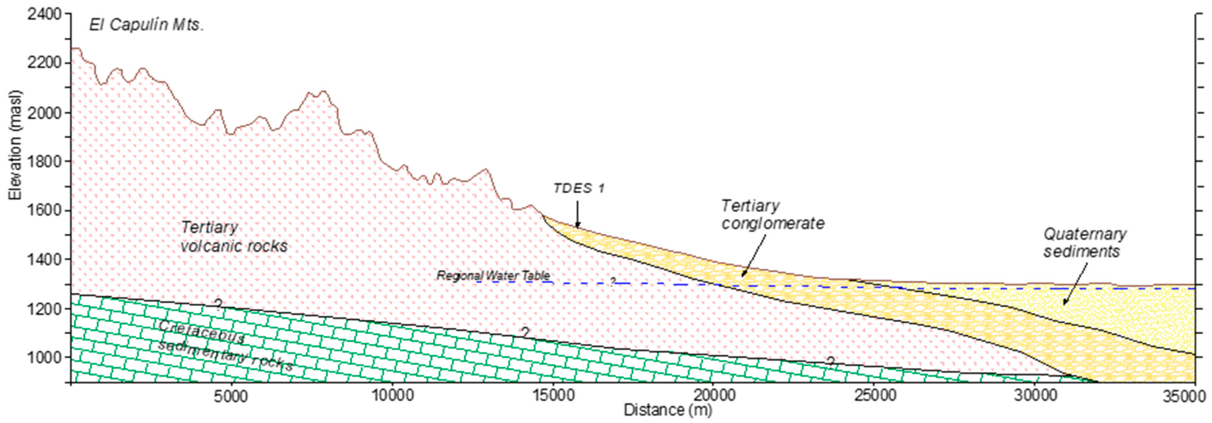
2.2. Structural Geology

The structural geology of the study site is relevant to understanding the aquifer settings, potential recharge, and groundwater flow. The youngest rocks that outcrop in the area are alluvial deposits from the Quaternary age (Qal < 10 thousand years), which were formed by fragments of weathered rock derived from the mountain fronts that define the watershed divide of the basin. These deposits include sand, silt, and clay in different proportions from erosion, which are subsequently deposited by streams and within the paleolacustrine system of the Laguna San Juan. Intermontane basins of the Basin and Range (B&R) province, Mexican Highland Section (MHS), have three major landscape components: piedmont slopes, basin floors, and river valleys. Piedmont slopes comprise:

(1)

Narrow erosional surfaces (rock pediments) adjacent to mountain fronts;

(2)

Broad fan-piedmont surfaces formed by coalescent alluvial fans or by alluvial slopes without distinctive fan morphology [13].

From the end of the Tertiary period (>5.1 Ma [Ma = millions of years]), conglomerates (Tcg) were formed by clasts larger than the alluvium, reaching sizes as large as boulders located in the streams, together with a poorly classified matrix of silt, sands and clays. The mountain ranges are composed of Tertiary age rocks from an alternation of rhyolite spills with acid tuffs (Tom(R-Ta)) and significant thicknesses of ignimbritic tuffs (T(Ti)) and acid tuffs (T(Ta)) outcropping the mountains. Towards the east, outside the area covered by the geological plane, sedimentary rocks of the Cretaceous age (>65 Ma) appear, which form the basement of the tertiary volcanic sequence that dominates the study area. The sequence of Cretaceous age sedimentary rocks was initially affected by compressive tectonic forces that caused reverse-type faulting as well as large folds that gave rise to the anticlines and synclines present in the Sierra Boca Grande to the northeast of the study area (Figure 4). Subsequently, the entire stratigraphic sequence has been subjected to stresses that have given rise to normal-type faulting and fracturing during the stage of intense volcanism. The stresses also generated faulting and fracturing in the pre-existing rocks, especially due to the thrust efforts of the magmatic chambers, which might have generated secondary porosity for groundwater to flow through these fractures [15].

2.3. Mapping “Water by Air”

Mapping “Water by Air” applies specifically to groundwater studies using satellite imagery and aerial photography. In this method, various spectral techniques are exercised using satellite images as the main input. The procedures for this approach were initially proposed by a group of researchers led by Gold and Parizek [12], in which lineaments and fractures were identified by spectral manipulation. Before going out into the field, the first step in the investigation consisted of carrying out a geostatistical calculation using principal component analysis (PCA) to identify the potential lineaments and fractures. This statistical manipulation is commonly used to reduce redundant spectral value pixel data of satellite images that have a large volume of digital datasets by creating a smaller dataset yet preserving most of the valuable information contained in the larger set. This method allowed us to locate points of intersection of faults and lineaments, which could be related to areas of greater potential for detailed exploration for groundwater, thereby serving as a basis for potential success in drilling groundwater wells [12]. Moreover, these geomorphic features allow mapping of the distribution of lithological units, drainage systems, surface water sources, soil moisture, and vegetation patterns, all of which assist in the hydrogeological characterization of a project area and increase the potential for successful drilling of a groundwater well from 25% to 75% [16].

For this study, satellite images from the LANDSAT 8 platform, obtained from the U.S. Geological Survey (USGS) online server, were used [17]. The images were selected based on the oldest date and clearest skies possible to rule out any visual alterations in the terrain, as well as to create a better-quality representation of the study area in terms of its geomorphology, thus increasing the possibility of detecting faults and geological lineaments. Because the studied area is an unaffected terrain with preserved natural conditions and limited anthropogenic influence, the dates considered were 29 June 2021, 27 August 2021, and 9 September 2021, which had good quality imagery with less cloudiness. Older imagery was not required.

Once a satellite image was selected, PCA was applied using Esri ArcMap GIS software to eliminate fuzzy digital data within the satellite image from matrix projections. The digital procedure was performed on the pixels of the image (~30 m × 30 m spatial resolution), which were selected in a “kernel” matrix where the criterion was to select the eight neighboring pixels closest to the point of interest (“input”), and the spectral values of each of the immediate neighboring pixels were averaged to assign a new value to the one selected (“output”). From this procedure, the amount of information found within the original data of the satellite image was reduced, highlighting the main component with the most significant amount of information. Once PCA had been carried out on the imagery, subsequent filters were applied to the main component with the largest amount of data to highlight the characteristic pixels, or those belonging to the same data group. For this, a low-pass filter was applied, smoothing the data by reducing local variations and removing noise from the image. A high-pass filter was used to accentuate the comparative difference between surrounding pixels. In this way, fuzzy data were removed from the image and linear patterns within the terrain were highlighted for future observation. Once the application of subsequent filters to the main component had been carried out, an unsupervised classification of the image was carried out from eight spectral classes taken from cluster pixels with defined values. This procedure was used for the characterization and grouping of characteristic pixels within the image, classifying them within the assigned classes. The classes were assigned based on the spectral values and integrated into this “cluster” of spectral values (“input”), which were defined within the eight selected classes. This allowed the attenuation of the lineaments observed within the study area by considering topographic descents, which usually represented aligned valleys, runoff alignments, vegetation alignments, and soil tones [6,18].

Geological abnormalities and geographic features were identified on the processed satellite imagery by looking for linear features such as abnormal linear vegetation growth, minor topographic linear discontinuities, linear arroyos, linear ground depressions such as potholes, and aligned soil tones with darker spectral reflections, which were enhanced by digital computer processing. This technique has been used to estimate and indirectly map groundwater flow [12] and has been useful for the identification of potential well drilling sites in areas with a large concentration of geological fractures and lineaments [18]. Additionally, pumping well fields near fractures or their intersections can indicate a greater likelihood of the presence of groundwater [19]. Furthermore, data acquired through satellite images and remote sensors can provide information about changes in characteristics that influence geohydrological revisions, including analysis of water recharge using thermal images and multispectral and radar data [19]. Such geological abnormalities can be identified in processed satellite imagery by identifying enhanced linear features. Using these geomorphic linear features can reduce the risk of drilling a dry groundwater well. Furthermore, it has been documented that such groundwater infrastructure sitting at a fracture zone has higher yields and specific capacities due to its extended elongation, which can capture recharge from far away locations within a watershed [20].

In México, fracture trace analyses for groundwater assessments have been carried out in different locations. For example, in Nayarit, a study was completed based on the processing and interpretation of structural lineaments from LANDSAT images using computer programs for the application of band compositions and PCA, with the objective of highlighting the lineaments and fractures of the study area [21]. In the same way, the analysis of LANDSAT satellite images was applied in Baja California, Mexico, using a digital elevation model for the formulation of a cartography of the geomorphology and geology of the area to obtain structural features (lineaments and fractures) and identify recharge and discharge areas in the San José del Cabo Hydrological Basin [22]. Furthermore, investigations of lineaments and fractures have been carried out based on PCA analysis in the lower Casas Grandes River Basin using satellite images processed for the identification of linear feature structures [6,16,23].

2.4. Geophysical Surveys

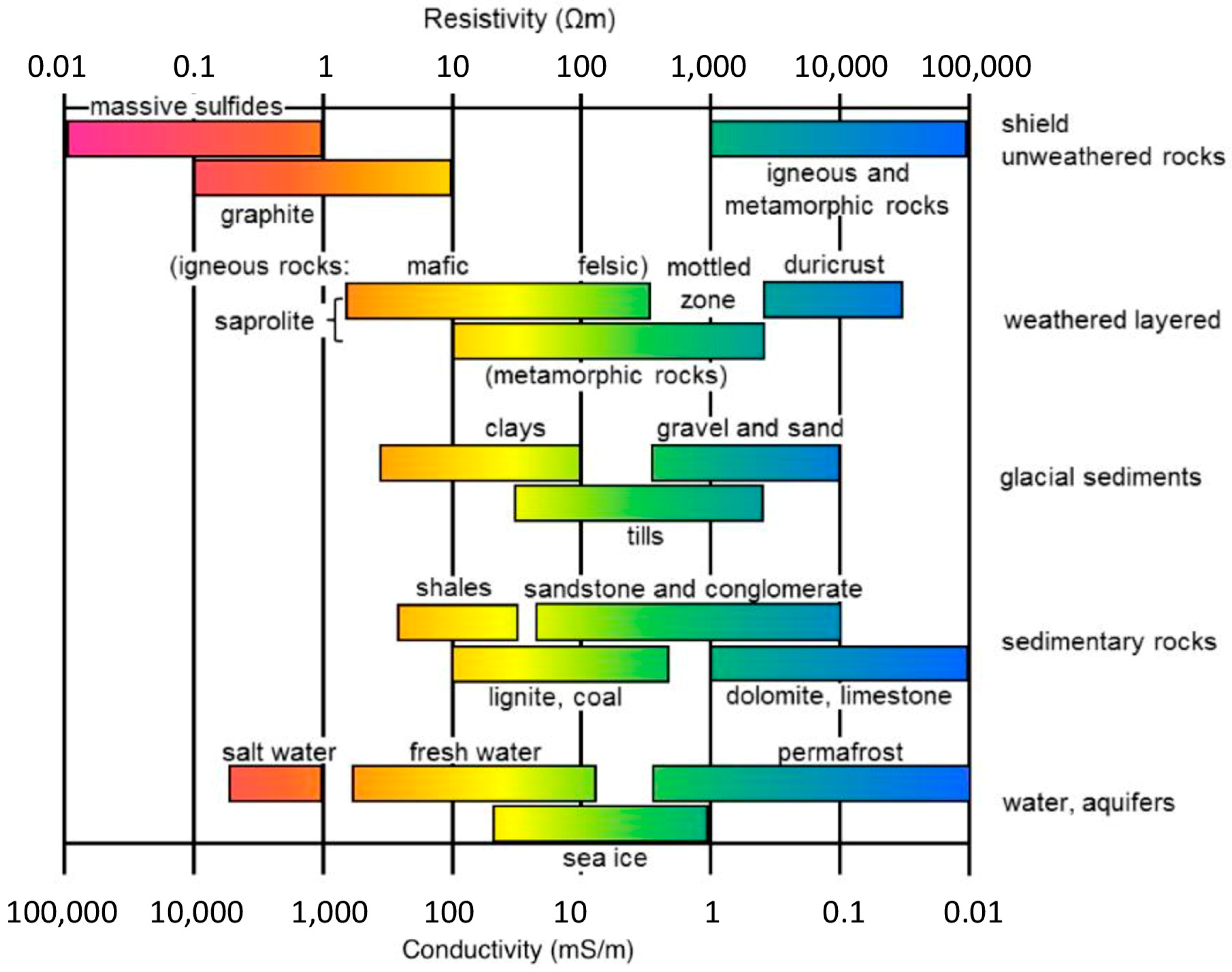
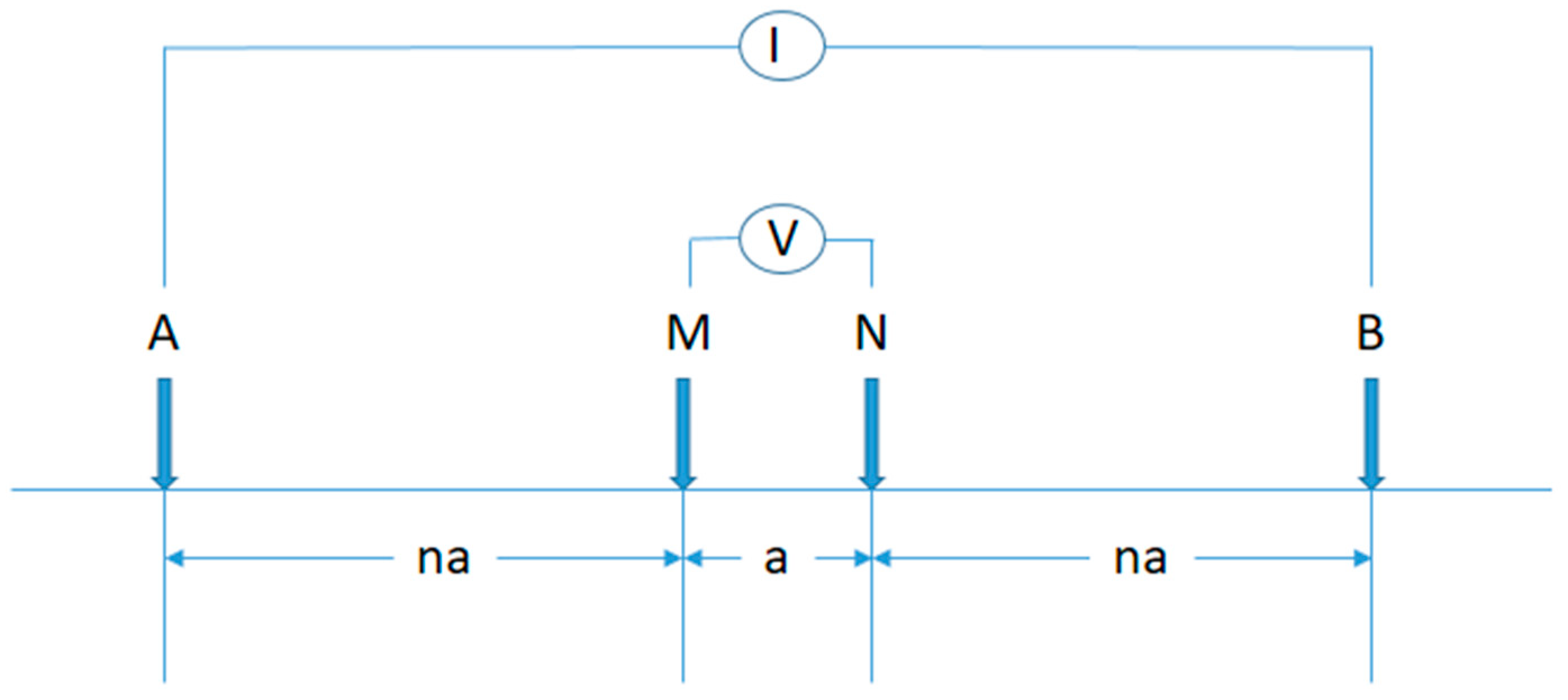
2.4.1. VES Theoretical Foundations

Although VES is not the only available method to test electrical resistivity, it is commonly used in groundwater studies [23,24]. The objective of the geophysical surveys in this study was to determine the distribution of electrical resistivities of the materials in the subsoil just under the identified lineament intersections. Based on the results of these geophysical surveys, we could assume the geological environment just below the chosen lineament intersection and later define if these values indicated a discontinuity in the geology that could be interpreted as a fault or fracture. VES is generally performed by applying a direct or low-frequency alternating current to the subsurface in order to differentiate various resistivities of the flow of electric current. These resistivities are indirectly interpreted as different types of geological materials or potential groundwater located in the subsoil according to their values (Figure 5). Surveys were carried out using a Ohmega Ω resistivity model equipped with a transmitter having a maximum power output of 36 W, a current range of 0.5 to 200 mA, a square wave repetition of 8.4, 4.2, and 28 s, and several readings averaged from 1 to 16. The model’s receiver was designed to have an input voltage range of 1–180 V with auto gain averaging.

The electrical potential is measured between two electrodes, through which an electric current with a specific voltage is injected into the ground. The arrangement of electrodes, known as the Schlumberger array, was a modification of the Wenner method [26] using four electrodes, but in this case the separation between the central or potential electrodes (a) remained constant, and the measurements were made by varying the distance of the outer electrodes from the inner electrodes at multiples (na) of the base separation of the inner electrodes (a) (Figure 6). The Schlumberger electrode display is very useful when it is necessary to know the resistivities of deeper layers because it does not require as many measurements as the Wenner method. The working principle is the same as the Wenner method; however, the Schlumberger method separates the outer electrodes progressively around an imaginary axis in order to determine the resistivity of the soil at greater depths (i.e., greater than 100 m). Inversion of the Schlumberger data was carried out using IX1D software [27], and the thickness and resistivity were left out because neither the thicknesses nor the resistivities of the materials present in the subsoil of the study site were known. There was no need for smoothing (shifting) or adjustment of overlap in the field curve because this was detected by the software and the adjustment (shift) was introduced in the calculations [24]. Variations in the electric current with respect to depth caused variations in potential difference measurements, which provided information about the subsurface structure and materials.

In general, a system of four electrodes embedded in the ground and symmetrically distributed is used in the geoelectric method for aquifer and hydrostratigraphic characterization. On the outside, two electrodes (A and B) are used to introduce electrical current into the subsoil. Two central electrodes (M and N) are used to measure the potential generated by the passage of the electric current in the subsoil at different depths, depending on the electrode arrangement of the terminals AB and MN (Figure 6). One of the electrical methods used in this investigation was VES modality, using the Schlumberger electrode array [27].

The mathematical expression for the calculation of the apparent resistivity in this Schlumberger electrode arrangement is given by:

ρ_α = ΔV/IK; where K = (2π/(1/AM − 1/BM − 1/AN + 1/BN))

(1)

where ρ_α is the apparent resistivity measured in Ωm; K is the geometric factor that depends on the electrode openings of the geometric arrangement of the electric current injection pins; ΔV is the potential difference; I is the current intensity in mA; A and B are the current electrodes; and M and N are the potential electrodes.

2.4.2. TDES Theoretical Foundations

The other geophysical method used for groundwater prospecting in this research was the TDES, which measures the decay of a transient secondary magnetic field by cutting off power to the transmission loop [27]. The secondary field generated by the flow of the induced current in the ground is measured by a receiving coil after the transmitted current is cut off. The stress of the secondary or transient field in the first-step window gives information about the conductivity of the shallow subsurface, whereas the transient stress in the last-step window is influenced by the conductivity of the subsurface at depth. Each survey carried out gives punctual information about the horizontal plane and only gives us information in the “Z” or vertical component. Comparing the information of several surveyed points in the horizontal plane and joining them as a profile allows us to analyze the information in depth and horizontally; that is, it produces an analysis in two dimensions. On the other hand, the lineament analysis carried out in this study aimed to locate the possible geological structures that could be identified on the surface through this methodology, thereby giving spatial information in the horizontal plane. With the soundings carried out in this study, it was possible to determine a difference between the subsoil resistivity values in the vicinity of the lineament (TDES1) and the subsoil resistivity values at the selected site with overlapping lineaments (TDES2). Both TDES1 and TDES2 were interpreted using the TemMerge module of WinGLink software to average the data with the same frequency and filter the points or windows with high errors, to generate the input file for the inversion [28]. From the assessed information, the depth and spatial information could give a certain degree of validity to a geological-structural analysis in which the geometry corresponded to a problem in three dimensions and the degree of certainty could increase with a greater number of probes.

Geoelectric and geological cuts differ in that the latter has limits in the separation of layers in the terrain, while the former only reflects changes in resistivity. The limits of both may or may not coincide. As an example at the same stratigraphic level, two or more layers can be found with different resistivities. This may depend on the degree of saturation of the rock and of the mineralization of the potential waters that permeate it. Sometimes the opposite is observed: layers of different compositions and ages behave electrically as a single homogeneous layer; hence, the number of layers and their separation limits can be different in geological and geoelectric sections [28]. The waveform of the secondary magnetic field (induced current) is generated by the interruption in the flow of electricity in the loop or transmitter frame. The active period between time on and time off (ramp time) and the measurement period after cutting off the current flow (time off) are the measurement times during which sounding records are obtained. There were 25 decay curve windows for the readings taken with a frequency of 16 Hz, and 22 for 32 Hz. The time domains are in the current and there is a “ramp time” in the primary magnetic field between “time on” and “time off” to later manifest the current of the magnetic field resulting from the induced current and the measurement windows along the path of a time end measurement. This method allowed the resistivities of materials to be identified at different depths in the lithological section of the study zone [29]. The type of arrangement used was “in loop” and three repetitions were carried out for each frequency used (stacks). The measurement frequencies, windows, and cycles used during the electromagnetic surveys are shown in

Table 1. TDES frequencies, windows, and cycles.

Frequency (Hz)	Windows	Cycles
32	22	1024
16	25	1024
8	28	512

.

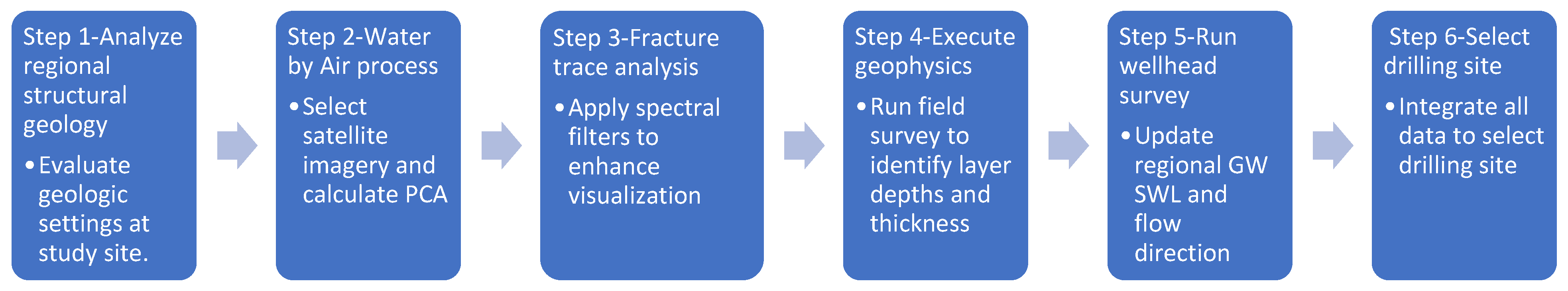
2.5. Initial Screening to Streamline the Field Investigation

Spectral analysis of satellite imagery to enhance the visual and digital interpretation of lineaments was carried out using a computerized process. The geostatistical interpretation calculated a matrix of statistical values identified as eigenvalues, to highlight the main component. A process of applying subsequent spectral filters to the satellite image was used to better visualize the linear features of the terrain, which facilitated interpretation of the lineaments and fractures within the study area. Unsupervised classification of eight spectral classes, selected from the databases obtained from the digital filters, was then applied. Once the geostatistical processing of the satellite image was completed, the “Water by Air” methodology was carried out, in which the analysis of lineaments and fractures was visually compared with the geological faults identified by the official Mexican geological cartography, reported by the Mexican Geological Service (SGM) [30].

Specific geographic points for the geophysical analysis were selected from the lines representing fault crossings and lineament intersections identified in the PCA during the spectral mapping procedure of “Water by Air”. Next, we carried out fieldwork with these geographic coordinates, identifying several geologic and geomorphologic features that were visually associated in the field with the spectrally mapped lineaments. Some of these geomorphic features were related to ruptures in topographic slopes; straight segments; abrupt changes in runoff alignments, linear ditches, and tributary valleys that were oblique to the local topographic slope; slightly taller aligned vegetation reflecting differences in growth response in dry seasons; linear zones with increased weathering of parent rock; linear zones with increased fracture and joint density; and linear zones of increased source rock permeability. This field recognition validated the sounding points to run the geophysical analysis gathering the resistivity data on the underground geologic materials at the survey sites. A graphical display of these values on a double logarithmic graph showing resistivity values and their subsequent geological interpretations was obtained. This information required a pre-interpretation process, which consisted of a displacement and/or adjustment of a “slight smoothing” calibration process of the gathered field resistivity curve in which new values of apparent resistivity were obtained. Finally, the calibrated resistivity values were processed using IX1D software for the final interpretation [27]. Additionally, a digital elevation model (DEM) of the study area was used to understand the dimensions of the basin under consideration, identify the main drainage network in the basin, as well as determine the exact location of groundwater wells in the study area.

Two VES and two TDES sounding surveys were carried out in the study area (Figure 1). The maximum opening (AB/2) was 320 m for VES1 and 400 m for VES2. The surveys were carried out using the Schlumberger modality. TDES1 was carried out near a previously drilled well. The distance between the well and the TDES1 site was 30 m, and the well did not have any electrical equipment. There were no nearby power lines that could interfere with the measurements. TDES2 was carried out at the same point as VES1, showing groundwater possibilities based on the “Water by Air” mapping procedure, so that the TDES soundings could verify the geoelectric units defined by VES1. A current of 10 Amp was applied in a 100 × 100 m box for a dipole moment of 100,000 Ampm² for the TDES soundings.

2.6. GPS RTK Wellhead Survey

Differential GPS positioning and elevations were determined at well locations to provide up-to-date piezometric levels of the area. A 220-channel Rover STONEX S9, UHF radio modem, and dual-frequency GPRS equipment were used to perform an RTK survey. The survey mode was fast static (static vertical accuracy: 10 mm ± 2 ppm), which required post-processing against a Continuous Operating Reference Station (CORS), and a RGNA (spanish acronym for Active National Geodetic Network) base, or reference station. The base station was left at the point defined as CAST (Castañeda site) and was in operation during the field survey. Subsequently, the survey was carried out with the base and mobile GPS RTK Trimble Unit. Throughout the survey, the base station collected data to process the records acquired with the mobile GPS receiver (rover) for at least 20 min. The precise locations (~2 cm in X–Y; ~2–5 cm in Z) of the surveyed groundwater wells were then used to determine the elevation at the well location. During the rover data collection, the static groundwater level in the surveyed wells was measured using a Solinst Water Level Meter Model 101 to estimate the precise depth of the static groundwater level in each of the wells.

The procedure and strategies to achieve improved placement of groundwater wells for livestock are presented in Figure 7. The proposed workflow is a multi-task approach for GW exploration that aims to identify fault intersections [12].

3. Results

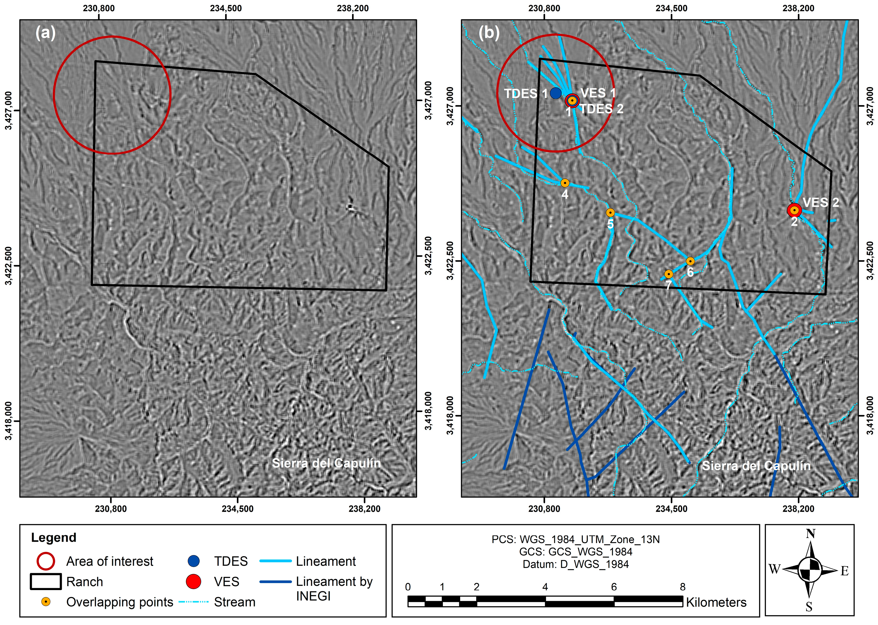
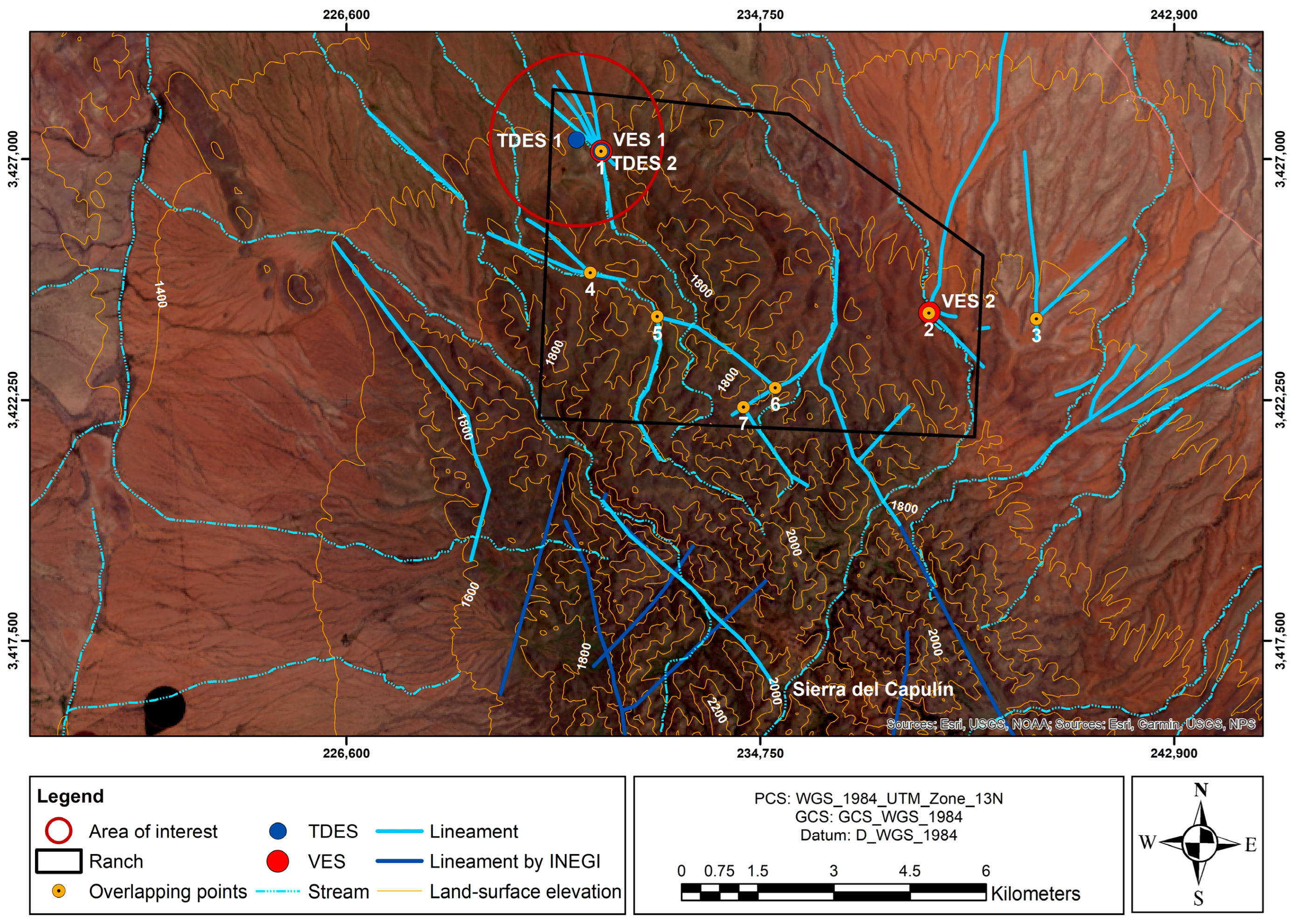
3.1. Interpretation of PCA

In this project, the digital information obtained from the spectral values of images from the LANDSAT 8 satellite was manipulated, resulting in the enhancement of geologic lineaments that were overlapped with the lineaments documented by the mining geological chart H13-4 published by the Mexican Geological Service and INEGI (National Institute of Statistics and Geography) [29]. The resulting images obtained with the spectral procedure allowed the identification of lineaments and fractures within the study area based on the “Water by Air” methodology.

The principal components that were obtained through the process of calculating the roots and characteristic vectors of a symmetric matrix contained most of the observed variance, separating most of the repeated information within the analysis. In the interpretation, the mapping of linear features associated with lineaments and fractures was carried out on different images with different wavelengths. This mapping is an important tool with respect to groundwater exploration in metamorphic, igneous, and karstic-sedimentary terrains because most of the water is found near fractures where the greatest permeability and porosity is found [31]. The PCA procedure generated eigenvalues, which statistically highlighted the main components corresponding to the greatest amount of spectral information. Within this statistical analysis, the main component (PCA1) contained 87.36% of the total spectral data of the satellite imagery, which was used to evaluate the possible points to explore in the field (

Table 2. Correlation of eigenvalues for PCA.

PCA Layer	Eigenvalue	Percentage of Eigenvalues	Accum. of Eigenvalues
1	13,360,881	87.36	87.36
2	1,016,952	6.65	94.01
3	667,394	4.36	98.37
4	164,175	1.07	99.44
5	69,657	0.45	99.89
6	12,985	0.08	99.97
7	1462	0.03	100

). Once the PCA was completed, subsequent spectral filters were generated to eliminate noise and attenuate the main component achieved by highlighting the satellite images in relation to the enhancement of faults and lineaments. The application of these spectral filters allowed a better visualization of the linear characteristics, facilitating the interpretation of lineaments and fractures within the study area. Once this step was finished, an unsupervised classification was carried out, which defined eight spectral classes to explore. This spectral classification highlighted characteristic pixels for later interpretation. After the processing of the satellite images was complete, the analysis of lineaments and fractures was carried out with respect to the “Water by Air” methodology, verifying their correlation with geological faults reported by SGM INEGI [30] (Figure 8 and Figure 9).

The PCA analysis yielded a total of 26 lineaments within the study area, with a total of 7 overlapping points of interest for geophysical field exploration and/or as sites for groundwater recharge potential (Figure 8 and Figure 9 and

Table 3. Locations and elevations of points of interest for geophysical exploration developed by the fracture trace analysis. Locations in the Universal Transverse Mercator (UTM Zone 13N) projection.

Point ID	North (UTM)	East (UTM)	Elevation (masl)
1	3,427,155	231,615	1530
2	3,423,970	238,084	1619
3	3,423,851	240,192	1623
4	3,424,764	231,394	1638
5	3,423,891	232,720	1694
6	3,422,487	235,050	1682
7	3,422,105	234,424	1720

). These points of interest, which corresponded to intersections between the extended lineaments and identified faults published by other workers and by field validation, indicated potential groundwater conduits [18,23]. The trends displayed within the area of study showed the main direction of the lineaments and faults had a NW-SE orientation and NE-SW trend (Figure 8 and Figure 9 and Table 3).

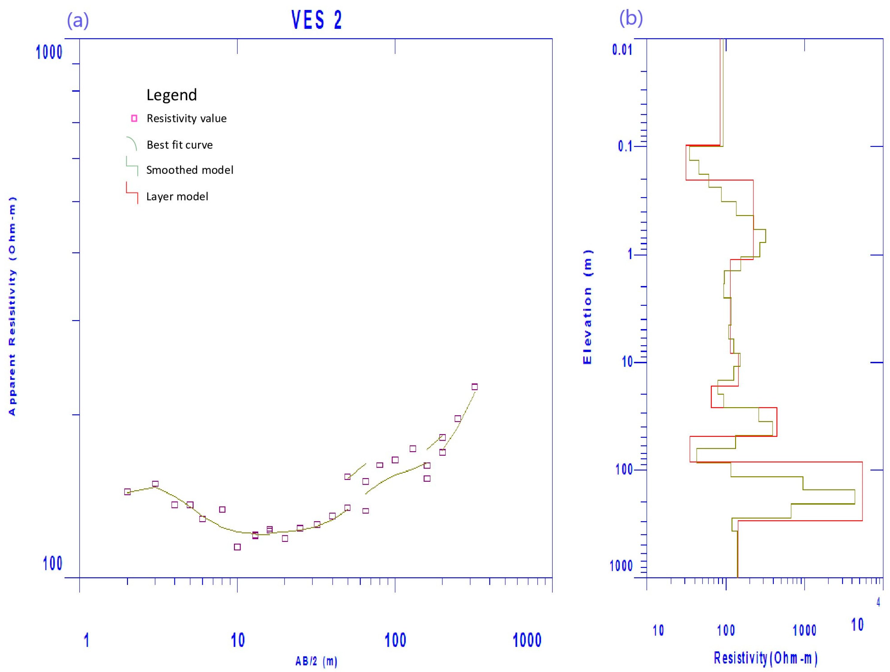
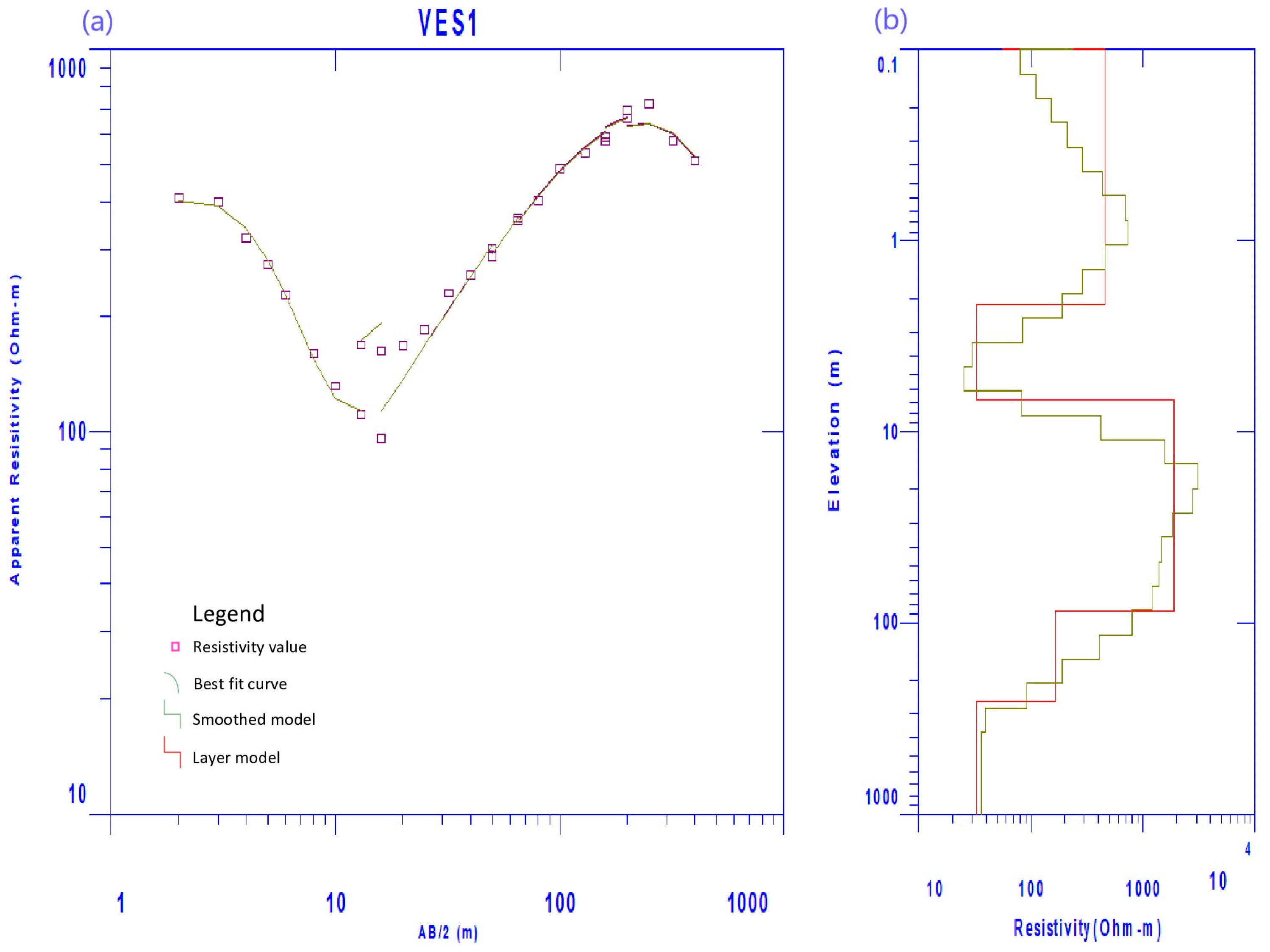
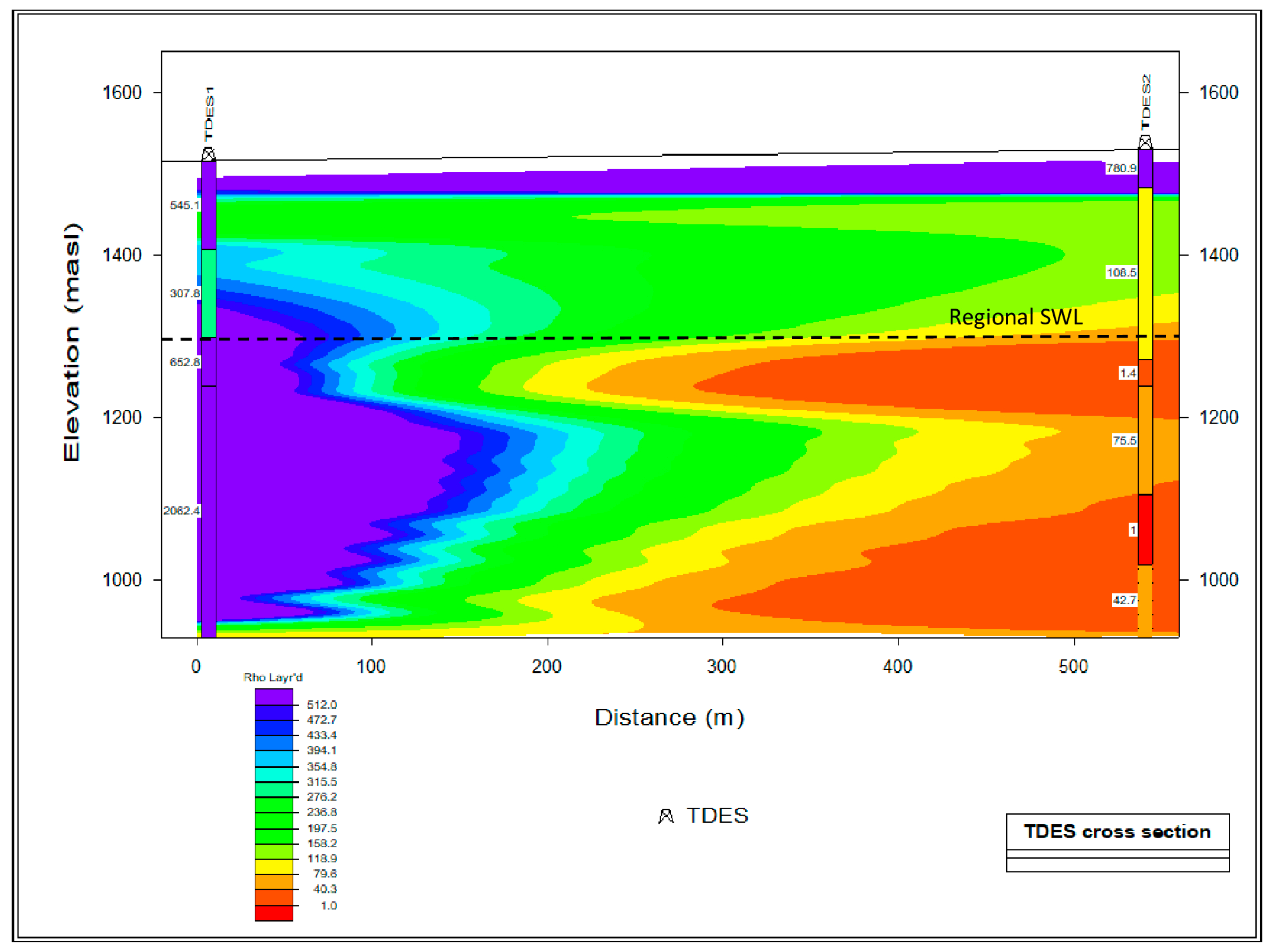
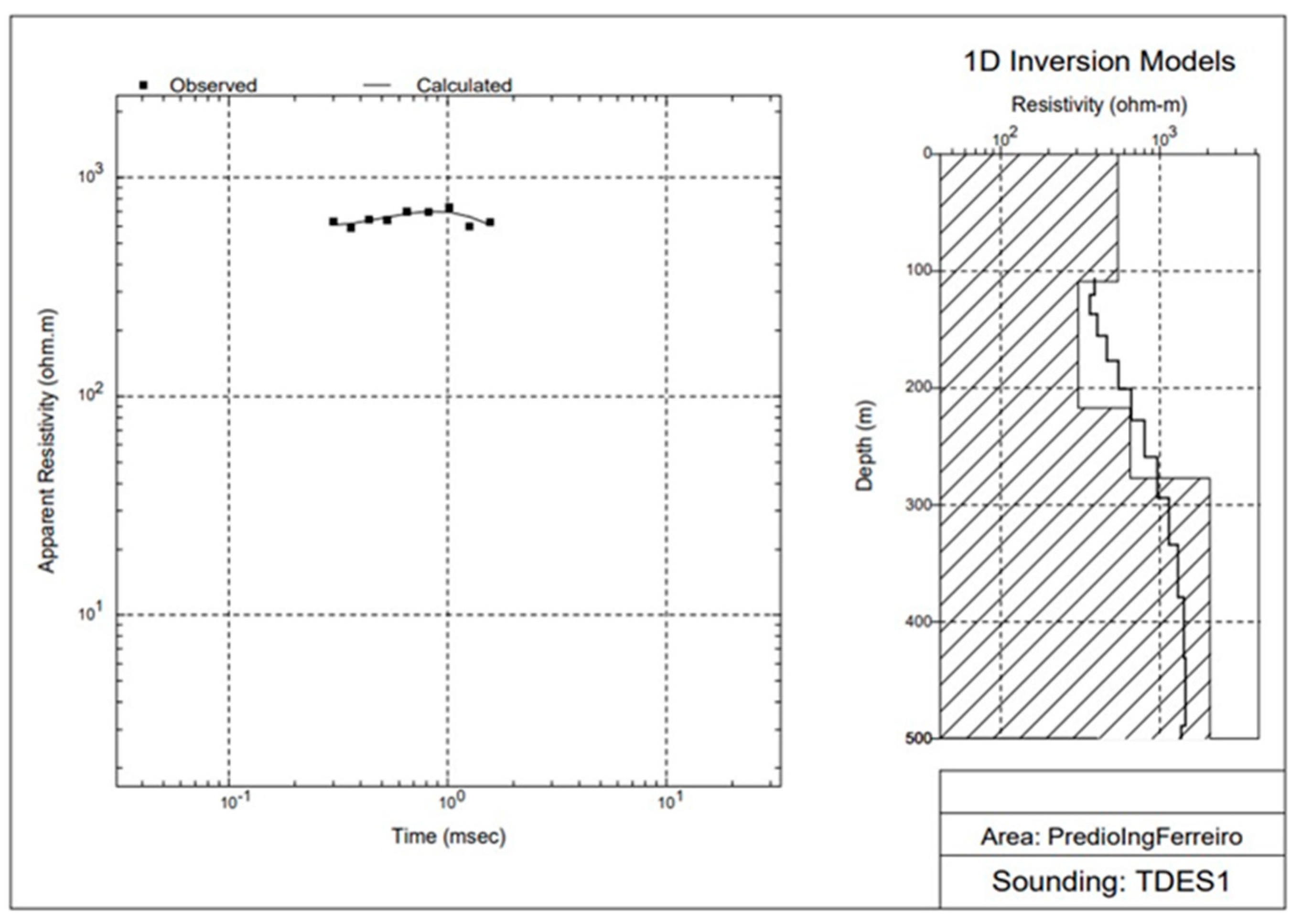
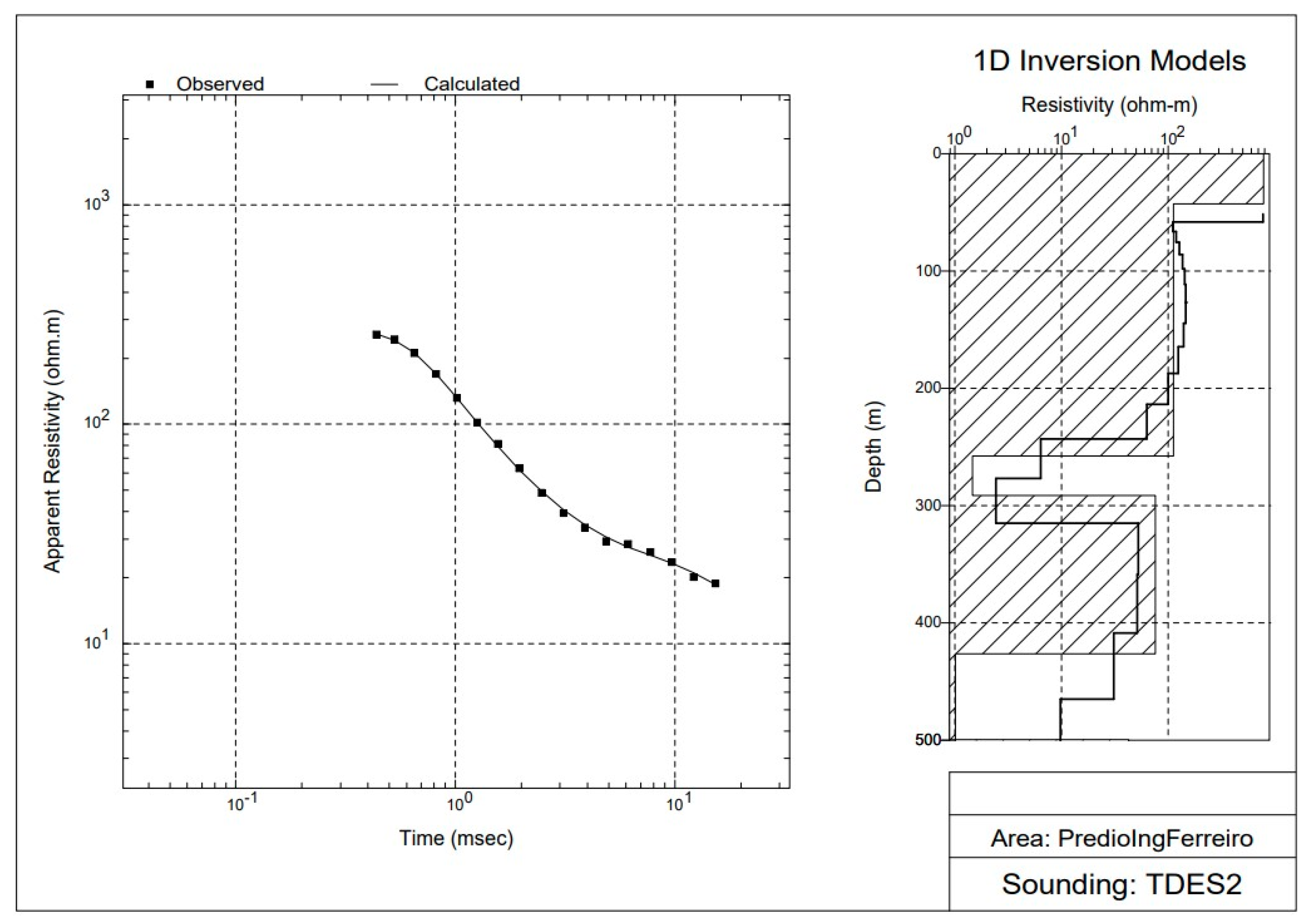
3.2. Interpretation of VES and TDES

The interpretation of VES and TDES data was accomplished by identifying the number of lithological units and their approximate resistivity values while estimating the survey field data, where a smoothed model was generated with specific software for each method (IX1D for VES and WinGLinK for TDES). Subsequently, the layered models were defined using inversion to minimize the error between the field data and the model. The error for VES1 was 4.52% and less than 1% for TDES2. A layered lithological model was established, and the direct solution could be automatically adjusted within the applied interpretation software IX1D [27] to fit the observed data. Neither thickness nor resistivity were manually fixed; rather, a smoothed model was generated. Based on this smoothed model, the layers in the models were defined and thicknesses and resistivities were left out when making the inversion, thus minimizing the root mean square (RMS). The second interpretation consisted of using the inverter of the interpretation software to fit the smoothed field curve with the best fit of the hydrostratigraphic model. Both methods reduced the possibility for error in the interpretation.

Interpretation of the field data generated by VES was represented by a curve of best fit and the layer model. The VES field data and curve of best fit at VES2 are presented in Figure 10. In the VES2 sounding, the small boxes with the magenta color (Figure 10a) represent the resistivity values obtained in the field for each spacing of the current electrodes (AB/2). The maximum opening (AB/2) was 400 m for VES1 and 320 m for VES2, and there were three segments of curves with overlaps between 13 and 16 m, 50 and 65 m, and 160 and 200 m. The openings for the potential electrodes (MN/2) were 5, 20, and 50 m. For the interpretation of the VES data, the software first generated a smoothed model of 30 layers from 0.1 to 500 m in depth. Based on this smoothed model, the layered model was built with thicknesses and free resistivities, running the inverter to minimize the error to RMS 4.52% for VES1 and 7.78% for VES2. There were also 38 equivalent models that fit the field data with different thicknesses and resistivities; however, the curve that presented the lowest RMS was selected. The options for smoothing (shift) the field data before inversion were “shift to match long spacing data” and “shift synthetics” to match original data [29].

The values obtained from the field work were represented by lithology segments showing the subsoil model, with the approximate thickness (m) of the layered materials on the y-axis and the resistivity values (Ohm-m) of these materials represented on the x-axis. The thickness and resistivity values are presented for two vertical electrical surveys carried out in the area (Figure 10a,b and Figure 11a,b). As explained above, the continuous magenta line represents the curve of best fit, in which a smoothed model displayed the parameters showing resistivity values and thicknesses of the surveyed strata. The VES2 results in Figure 10 showed resistivities as low as 35 Ohm-m starting at approximately 50 m to over 85 m in depth, indicating the potential for shallow subsurface groundwater flow that could provide water for livestock. It is important to highlight that groundwater flows might be present in the area where a drilling depth of approximately 85 m would be enough to capture potential water from the fractured system at the specific geographic point defined in this site. According to the stratigraphy of the study area, specifically in the area where the VES1 and VES2 surveys were carried out, a thin layer of sediments that corresponded to the piedmont conglomerate covered the sequence of rocks of extrusive igneous origin of intermediate to acid composition, such as tuffs, rhyolites, and ignimbrites, and also sedimentary rocks of the Cretaceous age located towards the base of the igneous sequence. According to this stratigraphy, a thin package of conglomerate with relatively high resistivities was present at a greater depth, which indicated rocks with reduced permeability. Nonetheless, the site’s geologic nature may vary according to the content of different materials, such as the alteration of tuffs, or the presence of secondary porosity, which could influence the groundwater flow captured from the headwater on the watershed.

In the case of the TDES2 sounding, the resistivities were associated with a discontinuity in the massive and compact rock sequence compared with TDES1, and a resistivity cross-section was constructed with the surveyed TDES. A discontinuity of resistivity values between both sites can be observed in Figure 12. The site where TDES2 was surveyed, which corresponded to the mapped cross lineaments at site 1 (Figure 13), showed stratified lower resistivity values, which could be associated with deposits such as conglomerates, alluvial deposits, or rock with intense fracturing, thus having a good possibility of groundwater production in between the high resistivity values. This discontinuity may be due to a fault that was identified as a lineament in the fracture trace analysis process, which can be attributed to intense fracturing caused by the stratigraphic unit. These fractures may be saturated with groundwater, which could be recharged from the upstream aquitards captured from vertical infiltrated runoff from headwaters on the watershed. Furthermore, there was a second layer of low resistivity values deeper than approximately 200 m and separated from the shallow layer by higher values. This intercalation of the two layers of deposits could indicate conglomerate-type materials separated by pyroclastic material from an intrusive volcanic eruption. The resistivity layer between depths of 85 and 200 m was above 5000 Ohm-m, which corresponded to rock with little or no permeability (Figure 10b).

Data at VES1 indicated a thin stratum with relatively low resistivity values present within the first 8 m but increasing to above 1700 Ohm-m to a depth of 95 m (Figure 11). From this point, the values of resistivity were reduced, reaching 193 Ohm-m at a depth of 192 m and further lowering to 34 Ohm-m at a depth of 240 m (Figure 11b). It is possible that some lithological sections at this site corresponded to volcanic rock with different degrees of fracturing, and the deepest stratum may be the sedimentary rock basement or fractured rock, which was defined as one of the points to explore for a groundwater well. However, a non-functioning well close to TDES1 was previously drilled to a depth of approximately 244 m and showed no groundwater potential; the same geologic unit continued to a depth of 278 m (Figure 14).

For confirmation of the results of VES1, an additional survey, TDES2, was carried out (Figure 15) at the same site as VES1. The TDES2 results showed substantially improved characteristics for the occurrence of groundwater. At this site, there was a low resistivity lithological section that had its base at a depth of 290 m and continued with low resistivity values of 75 Ohm-m for a total thickness of 134 m. The resistivity values of this unit indicated that it was likely to store and be capable of releasing groundwater through the siting of a groundwater well at this location (Figure 15).

The inversion models were developed by first generating a smoothed model with a maximum of 20 layers and an investigation depth of 58.3 to 602.8 m, calculated by the software. Based on this, the layered models were defined. These inverted models were used to generate the final thicknesses and resistivities of each site (the hatched areas on the right sides of Figure 14 and Figure 15 represent the final model of the inversion). For these data, since there was no point for calibration, the thicknesses and resistivities were left unfixed under the interpretation software. The parameters for the inversion were RMS < 5.0%, with 10 interactions [27].

The results for TDES1 showed high resistivity values which corresponded to a low potential for a permeable layer or a fractured geologic system that could imply the existence of any groundwater. Furthermore, these resistivity values corresponded to unaltered parent material, such as solid rock of volcanic nature or Cretaceous age sedimentary rock, as presented in the schematic interpretation in Figure 16. Blue dotted line with question mark represents the potential extension of regional SWL. Questions marks are plotted at the potential lithological contact between the Tertiary volcanic rocks and the Cretaceous sedimentary rocks.

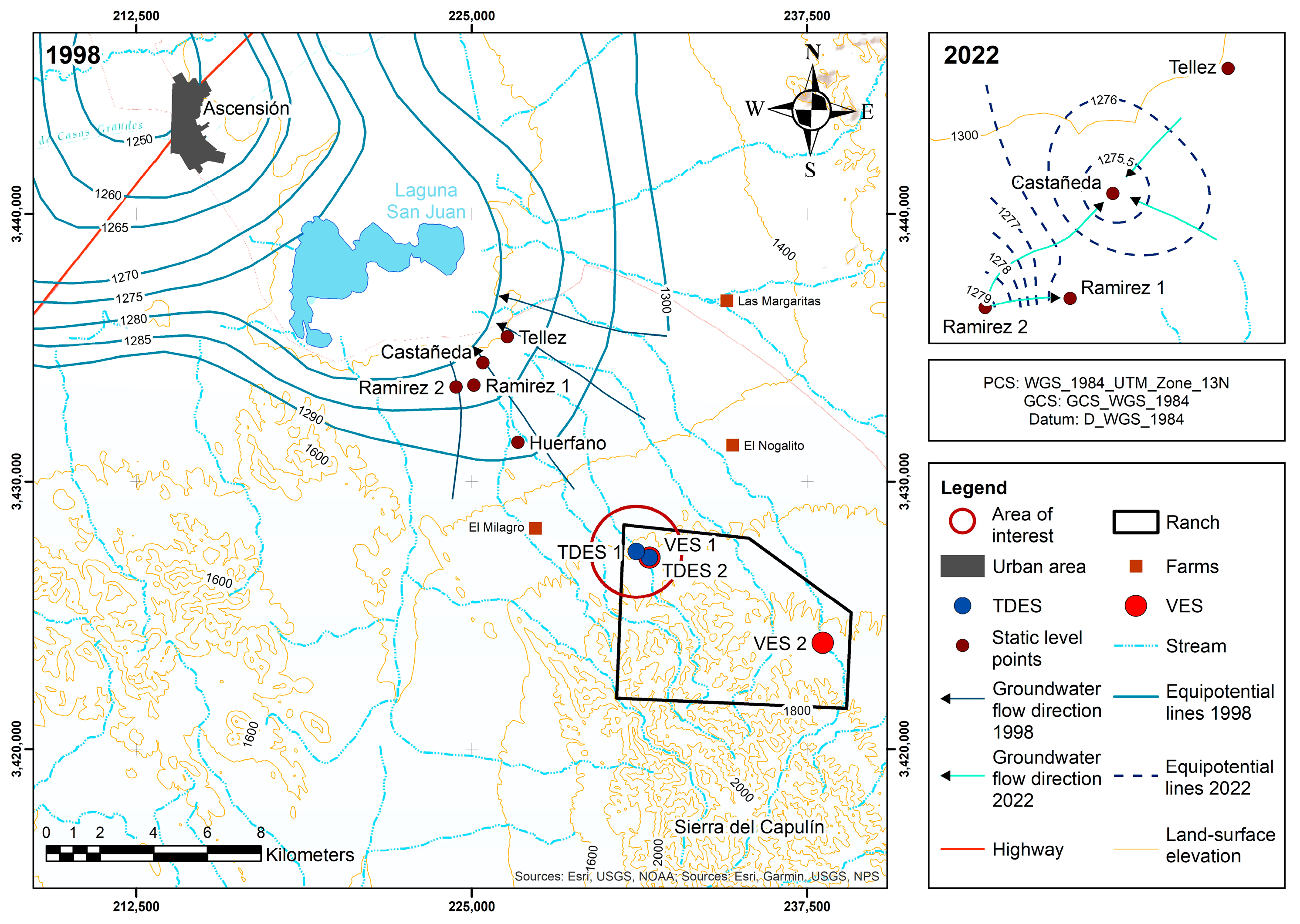
3.3. Piezometric Surface Construction

The application of geohydrological analysis to define groundwater potentials is fundamental to understanding the groundwater flow, and it can be complemented by the geophysical determination of the hydrostratigraphic units (HSUs) in a watershed. This allowed us to locate sites with the best possibility of having a saturated strata or geological formation for use in establishing an economically feasible groundwater well. To determine the groundwater potential of the various HSUs at the study site, a geohydrological analysis was carried out and a schematic diagram was created by surveying the geological formations and evaluating their possibility of receiving water from some source, either by recharge of pluvial origin or from groundwater flows from regional aquifers (Figure 16). To achieve this objective, it was necessary to carry out a topographic survey to generate static water levels (SWL) in order to model equipotential lines of groundwater flow for a battery of wells in the region. From this procedure, it was possible to define SWL at the points where the piezometric data were taken and map the networks of these equipotential lines of the subsurface flow and groundwater level for the regional aquifer.

3.4. Update of Equipotentials and Piezometry

The RTK survey of wells was completed using the Municipal Institute of Research and Planning (IMIP) base station in Ciudad Juárez, Chih., and the INEGI stations installed in the City of Chihuahua and in the City of Hermosillo. A constellation of 12 to 18 satellites was used to acquire a position at the points of interest, and at each site, the mobile GPS took readings for 20 min to link it to the base station sited at the Castañeda location. In total, position coordinates of five wells were obtained, as well as the 2022 depth to SWL (

Table 4. Real-time kinematic survey of wellheads and piezometry. Locations in Universal Transverse Mercator (UTM Zone 13N) and elevations in meters above sea level (masl).

ID	UTM East	UTM North	Elevation (masl)	Wellhead (masl)	Depth to SWL (m)	SWL (masl)
Base	222,601	3,434,253	1304.96	-	-	-
Castañeda	225,570	3,434,241	1305.92	1305.92	30.65	1275.27
Tellez	226,882	3,435,078	1307.39	1397.39	31.05	1276.34
Ramirez 1	225,222	3,433,380	1314.38	1314.38	38.15	1276.26
Ramirez 2	224,656	3,433,338	1313.46	1313.46	34.4	1279.06
Huerfano	227,154	3,431,206	1361.65	1361.65	86.5	1275.15

).

Table 4 shows the UTM coordinates resulting from the baseline georeferenced process for the control station (the base in Table 4) located near the Castañeda well site, along with the resulting georeferenced coordinates of points that were positioned with the mobile GPS. The georeferenced coordinates were mapped using the WGS-84 datum with the GGM-10 reference geoid and in a geographic format, which were later converted to flat UTM coordinates. Figure 17 shows the equipotentials of updated SWL for 2022, demonstrating the depletion that occurred in the aquifer during the period from 1998 to 2022, which was approximately 7 m (30 cm of SWL depletion per year) compared to the latest SWL survey performed by CONAGUA in 1998. For our paper, we only monitored five wells for the updated 2022 SWLThe Ascensión aquifer has systematic groundwater evolution data from 1977 until 1998. According to the data on the evolution of the static water level from 1987–1998, the aquifer presents an average drawdown of −1.0 m/year. However, in the vicinity of the town of Ascensión, there are maximum drawdowns of −29.0 m (−2.4 m/year). The drops in groundwater levels in this area range from −5.0 to −29.0 m (−0.4 to −2.4 m/year), occurring as an elongated cone from south to north in an ellipsoidal shape, with a length of 25 km on its long axis and 15 km on its short axis (Figure 17). These drops in static water levels are due to the large extraction of groundwater and the concentration of pumping wells. In the updated survey (2022), the well at the “Huerfano” site had stopped pumping 24 h before the hydrocensus took place; hence, the depth to SWL was higher, it had not yet stabilized and recuperated from the pumping process, and it showed a deeper SWL (Table 4).

Considering the topographic elevation of the validated site for the location of a new well, an equipotential line was defined at 1530 masl in the area of interest. The depletion in the aquifer at this site was estimated to be 7 m compared to the 1998 hydrocensus. A probable drilling depth could be evaluated at this site to reach the level of the potential regional aquifer at the point of interest and take advantage of the potential recharge that is probably provided by the mapped crossing fault systems and lineaments. If it is considered that the last equipotential projected in 1998 towards the area of interest was 1290 masl, the depth of drilling must be greater than 247 m to enter the potential SWL of the regional aquifer in the area (Figure 15). Similarly, it is possible that during the drilling of this new well, shallower groundwater from rainwater recharge may be present from the remaining saturated zone of fractured rock identified during the exploration stage with the “Water by Air” and geophysical methods.

4. Discussion

Groundwater demands for different uses have increased over time in this region. Indeed, groundwater depletion in shallow aquifers has become an issue in many desert environments worldwide. Although the aquifer at the study site is largely comprised of primary porosity integrated with sand, gravel, and clay at different depths and in its tridimensional composition arrangements, there are other factors affecting its groundwater potential. For example, due to various geological events, such as intrusive volcanics, Tertiary age rocks, as well as sedimentary rocks of the Cretaceous age that are outcropping the mountains at the study site, secondary porosity is present in these rock types that may enhance the possibility for groundwater. Furthermore, towards the southeast of the study area at the Sierra del Capulín, several shear faults and lineaments are present due to compressional and distension effects. Consequently, the hydrogeological functions of these aquifers differ compared to normal layered sedimentary deposits. Moreover, these lineament features induce the potential for groundwater flow through their secondary porosity, which functions differently compared to normal granular aquifers, while improving their potential yields. Such geological abnormalities were identified in processed satellite imagery by identifying enhanced linear features, such as abnormal linear vegetation growth, minor topographic linear discontinuities, linear arroyos, linear ground depressions such as potholes, and aligned soil tones with darker spectral reflections, which were heightened by digital computer processing. Aiming at these geomorphic linear features can reduce the risk of drilling a dry groundwater well or increase the potential for a high-yield well with up to ten times the production of a well on a granular aquifer system. Furthermore, it has been documented that such groundwater infrastructure sitting at a fracture zone has higher yields and specific capacities due to its extended elongation, which can capture recharge from far away locations within a watershed. In this research, we demonstrated how the mapped linear features found in satellite imagery after spectral manipulation with the “Water by Air” methodology correlated with the surveyed characterization of lithological units mapped after the geophysical surveys. Moreover, the low resistivity layers found at shallow depths at the selected fault intersections might correspond to a different aquifer formation as compared to the regional SWL projection. We also demonstrated that when information on groundwater characterization is unavailable or limited, the multitask procedure is a functional tool able to reduce the risk of investment when drilling for groundwater resources. However, there are uncertainties when applying the technique related to the scale of pixel resolution of the satellite imagery since such fracture and lineament features are narrow and sites can be misplaced if validation with geophysics is not applied. Furthermore, to improve estimates when siting a groundwater well using this procedure, studies should include debris analysis from lithological sampling during the drilling process from surrounding wells to corroborate the defined HSUs at the drilling site. Moreover, once a groundwater well has been drilled using this procedure, geological samples from the drilling grid should be carefully monitored and an aquifer test should be performed to validate the efficiency of the technique and improve estimates of groundwater in complex geologic settings.

5. Conclusions

A spectral analysis of the geologic and geomorphic lineaments and fractures was carried out based on geostatistical analysis of the main components together with processing of satellite images to eliminate fuzzy data within sets of LANDSAT TM8 satellite images. The spectral processing and digital manipulation of these satellite images allowed the enhancement and visualization of linear features within the terrain under analysis, which allowed pixels with similar characteristics to be highlighted and classified. The “Water by Air” methodology identified a total of 26 lineaments and fracture traces within the study area, of which seven sites were selected as potential points with intersected crossings of faults for further geophysical field exploration. These intersections of lineaments and faults were considered the points of greatest potential for groundwater exploration by geophysical methods, reducing the time needed for fieldwork and evaluation while improving the chances of successful groundwater well drilling. However, a validation process, which is an important step in the selection of a site for drilling, is of relevant significance. Using all available information, such as the lithological data from a well drilled near the site of interest as well as official data from previously mapped linear features, could increase the likelihood of a successful result when drilling for groundwater wells.

Evaluation of the structural geology and the geophysics survey at the site of interest identified a complex geology with challenging hydrogeologic conditions. Parent materials found at the site presented high resistivity values, which were interpreted as rocks with low permeability potential related to HSUs that do not store or transmit water. However, telluric processes in the area produced compressive and distensive events of tectonic origin that caused faulting and fracturing in some regions in the existing rocks at the site of interest, resulting in secondary porosity at higher elevations on the mountain fronts. These geologic settings function as potential recharge areas that could generate flow of groundwater on upper sections of the predominant strata in the piedmont fractured system. Furthermore, the difference in the resistivity profiles between TDES1 and TDES2 indicated a discontinuity that could be interpreted as a fracture zone towards TDES2. This site was in a fracturing or faulting zone, as identified in the previous exploration studies using mapping of groundwater by the “Water by Air” method. According to the exploration methods used, including field methods to position and run the electromagnetic soundings as proposed by our main objectives in the research rationale, we identified the point where the VES1 and TDES2 soundings were carried out as having the highest probability of finding groundwater among the studied locations.

Additionally, a hydrocensus was carried out, georeferencing wellheads of the local well infrastructure to update the groundwater evolution for the regional aquifer and extend it upstream into the headwaters of the watershed, aiming at the area of interest. This procedure included SWL measurements at selected wells and redefining the equipotentials for the regional aquifer at the time when this study was carried out, extending the potential regional SWL into the area of interest. In general, the regional aquifer has dropped by 7 m from 1998 to the present, declining at a rate of 30 cm per year on average in the region where the wellhead survey was carried out. In correspondence with the geohydrological analysis and complementing the geophysical study in the area of interest, the SWL of the regional aquifer was located at a depth of approximately 247 m at the point indicated by the UTM coordinates obtained by the “Water for Air” method for exploratory drilling at this site. Lithological samples from the well during exploratory drilling at the proposed site could validate the technique in this setting. On the other hand, there is the possibility for groundwater at site VES2 due to subsurface flows present in the upper fracturing zone (from 50 to 85 m deep), which was supported by the geophysical results. This could be shallower than a depth of 247 m, as suggested by the regional aquifer at site TDES2. The aquifer test after the drilling process ends is the best indicator of the performance of the multi- technique approach in locating potential groundwater resources in such a geologically complex scenario.

In conclusion, the approximation towards groundwater prospecting using a multi-technique framework methodology was proven to be effective in the identification of a low resistivity subsurface layer, which could be related to potential groundwater resources in a complex geological setting, thereby reducing the risks and improving the possibilities of drilling groundwater wells that are economically viable. This procedure can be applied to other regions around the world where minimum or nonexistent data are a challenge and where complex hydrogeological systems are present.

References

1. Robertson, A.J.; Matherne, A.-M.; Pepin, J.D.; Ritchie, A.B.; Sweetkind, D.S.; Teeple, A.P.; Granados-Olivas, A.; García-Vásquez, A.C.; Carroll, K.C.; Fuchs, E.H.; et al. Mesilla/Conejos-Médanos Basin: U.S.-México Transboundary Water Resources. Water 2022, 14, 134. [Google Scholar] [CrossRef]
2. WWAP-UNESCO. Groundwater, Making the Invisible Visible. 2022. Available online: https://www.unesco.org/reports/wwdr/2022/en (accessed on 10 May 2022).
3. UNESCO. World Water Assessment Programme. 2021. Available online: https://en.unesco.org/wwap (accessed on 10 May 2022).
4. Rivera, J.J.C.; Schmidt, S.; Kuri, G.H.; Rivera, J.J.C. Agua: El Oro Invisible; Cuadernos para el Debate; Centro de Estudios Económicos, Políticos y de Seguridad: Mexico City, México, 2022; Volume 78, p. 96. [Google Scholar]
5. Rivera, J.L.M. Hacer florecer al desierto: Análisis sobre la intensidad de uso de los recursos hídricos subterráneos y superficiales en Chihuahua, México. Cuad. Desarro. Rural 2016, 13, 35. [Google Scholar] [CrossRef] [Green Version]
6. Gameros, C.I.R.; Olivas, A.G.; Hernández, O.F.I.; Mercado, M.H. Evolución piezométrica del acuífero Palomas-Guadalupe Victoria (0812) en la cuenca baja del río Casas Grandes, Ascensión, Chihuahua, México: Piezometric evolution of the Palomas-Guadalupe Victoria aquifer in the Lower Basin of the Casas Grandes River, Ascension, Chihuahua, Mexico. TECNOCIENCIA Chihuah. 2021, 15, e802. [Google Scholar] [CrossRef]
7. CONAGUA. Actualización De La Disponibilidad Media Anual De Agua En El Acuífero Ascensión (0801), Estado De Chihuahua. Ciudad De México, Diciembre 2020. 21 Pag. Available online: https://sigagis.conagua.gob.mx/gas1/Edos_Acuiferos_18/chihuahua/DR_0801.pdf (accessed on 10 May 2022).
8. CONAGUA. Estadisticas del Agua en México. October 2022. 360 pag. Available online: http://sina.conagua.gob.mx/publicaciones/EAM_2021.pdf (accessed on 10 May 2022).
9. Mayer, A.; Heyman, J.; Granados-Olivas, A.; Hargrove, W.; Sanderson, M.; Martinez, E.; Vazquez-Galvez, A.; Alatorre-Cejudo, L. Investigating Management of Transboundary Waters through Cooperation: A Serious Games Case Study of the Hueco Bolson Aquifer in Chihuahua, México and Texas, United States. Water 2021, 13, 2001. [Google Scholar] [CrossRef]
10. Gutiérrez, M.; Gómez, V.M.R.; Herrera, M.T.A.; López, D.N. Acuíferos en Chihuahua: Estudios sobre sustentabilidad. TECNOCIENCIA Chihuah. 2016, 10, 58–63. [Google Scholar]
11. Aguirre, L.V.; Ayala, A.O. Provincias Hidrogeológicas De México. Ing. Hidráulica México 1992, 7, 36–55. [Google Scholar]
12. Gold, D.P.; Parizek, R. Fracture Trace and Lineament Analysis: Application to Groundwater Resource Characterization and Protection; Penn State University: Centre County, PA, USA; National Ground Water Association (NGWA): Westerville, OH, USA, 1999. [Google Scholar]
13. Hawley, J.W.; Swanson, B.H. V Special chapter: Conservation of shared groundwater resources in the binational Mesilla Basin-El Paso del Norte region—A hydrogeological perspective. In Hydrological Resources in Transboundary Basins between Mexico and the United States: El Paso del Norte and the Binational Water Governance; UACH Editors: Chihuahua, Mexico, 2022; p. 325. ISBN 978-607-536. [Google Scholar]
14. Ferreiro-Maiz, P.; Ferreiro-Laphond, V.; Union Ganadera Local de Ascensión, Chihuahua, Mexico; Owners Ranch El Milagro; Ascension, Chihuahua, Mexico. Personal communication, May 2022.
15. Hawley, J.W.; Hibbs, B.J.; Kennedy, J.F.; Creel, B.J.; Remmenga, M.D.; Johnson, M.; Lee, M.M.; Dinterman, P. Trans-International Boundary aquifers in southwestern New Mexico: New Mexico Water Resources Research Institute; New Mexico State University: Las Cruces, New Mexico, 2000; p. 126. [Google Scholar]
16. Sander, P. Lineaments in groundwater exploration: A review of applications and limitations. Hydrogeol. J. 2007, 15, 71–74. [Google Scholar] [CrossRef]
17. USGS. Earth Explorer. 2022. Available online: https://earthexplorer.usgs.gov/ (accessed on 10 May 2022).
18. Granados-Olivas, A. Relationships between Landforms and Hydrogeology in the Lower Casas Grandes Basin, Ascensión, Chihuahua, México. Ph.D. Thesis, New Mexico State University, Las Cruces, NM, USA, 2000; 289p. [Google Scholar]
19. Meiser, E.; Earl, T. Use of fracture traces in water well location: A handbook. In Fracture Trace and Lineament Analysis: Application to Ground Water Resources Characterization and Protection; United States Department of the Interior: Washington, DC, USA, 1982; pp. 93–155. [Google Scholar]
20. Meijerink, A. Remote Sensing Applications to Groundwater, 16th ed.; UNESCO: Paris, France, 2007. [Google Scholar]
21. Carrillo de la Cruz, J.L.; Alcázar, F.D.J.E.; Camacho, A.Z.; Cornú, F.J.N. Interpretación de lineamientos estructurales en Nayarit, México, aplicando sensores remotos y software libre. GEOS 2015, 35, 351–358. [Google Scholar]
22. Martínez, G.; Diaz, J.J. Morfometría en la Cuenca Hidrológica de San José del Cabo, Baja California Sur, México. Rev. Geol. Am. Cent. 2011, 44, 83–100. [Google Scholar] [CrossRef] [Green Version]
23. Ramírez-Villazana, O.; Granados-Olivas, A.; Pinales-Munguía, A. Clasificación geoespacial de los indicadores del medio físico para la recarga del acuífero Palomas-Guadalupe Victoria, Chihuahua, México. TECNOCIENCIA Chihuah. 2016, 10, 32–38. [Google Scholar]
24. Spies, B.R.; Frischknecht, F.C. Electromagnetic Sounding; Investigations in Geophysics; SEG Library: Houston, TX, USA, 1991; pp. 285–425. [Google Scholar] [CrossRef]
25. Developers GeoSci. Typical Values for Rocks. DC Conductivity/Resistivity. 2018. Available online: https://em.geosci.xyz/content/physical_properties/electrical_conductivity/electrical_conductivity_values.html (accessed on 10 May 2022).
26. Wenner, F. A Method of Measuring Resistivity; Scientific Bulletin; National Bureau of Standards: Gaithersburg, MD, USA, 1915.
27. IX1D v3 Instruction Manual, 2007. Version 1.11 Copyright © 2007 Interpex Limited All Rights Reserved 22 March 2008 Interprex Limited P.O. Box 839 Golden CO 80401 USA. Available online: https://www.scribd.com/document/390680354/ix1dv3manual (accessed on 23 May 2022).
28. A guide to using WinGLink®. Release 2.20.02.01. Copyright © 1998-2008 by: GEOSYSTEM SRL. Printed in Milan, 10 January 2008. Available online: http://nebula.wsimg.com/6f5c6da1fd7f70a20b5e566761696b98?AccessKeyId=50358F51F2F2A243B87B&disposition=0&alloworigin=1 (accessed on 10 May 2022).
29. Kalenov, E.N. Interpretacion de Curvas de Sondeos Electricos Verticales; Ministerio de Obras Publicas y Urbanismo: Madrid, España, 1987; ISSN 84-7433-51 3-2. [Google Scholar]
30. SGM, Servicio Geológico Mexicano. Carta Geológico-Minera, Nuevo Casas Grandes H13-4, Chih. Revisado en línea: 04 ago. 2022. Available online: https://mapserver.sgm.gob.mx/Cartas_Online/geologia/34_H13-4_GM.pdf (accessed on 4 August 2022).
31. Vincent, R.K. Fundamentals of Geological and Environmental Remote Sensing; Prentice Hall: Hoboken, NJ, USA, 1997. [Google Scholar]
Figure 1. The reported 1998 equipotential lines and groundwater flow direction [7].
Water 15 01673 g001
Figure 2. Location of the Ascension aquifer in northern Chihuahua, México [7].
Water 15 01673 g002
Figure 3. Conceptual model of the structural geology at the study site. TDES2 represents the approximate location for a time domain electromagnetic sounding. Blue dotted line and question mark represents the potential extension of SWL.
Water 15 01673 g003
Figure 4. Regional geologic settings at the Ascension aquifer.
Water 15 01673 g004
Figure 5. Electrical conductivity and resistivity values for different rocks [25].
Water 15 01673 g005
Figure 6. Electrode arrangement for the Schlumberger configuration. AB represent the current electrode pairs and MN represent the potential electrode pairs; I is the current source and V is the volt meter; a represents the space between the moving MN electrodes and na represents the moving space in between the AB current electrodes.
Water 15 01673 g006
Figure 7. Workflow for a multi-technique framework for groundwater prospecting.
Water 15 01673 g007
Figure 8. Image of the study area after the application of spectral filters highlighting linear terrain features. (a) High pass filter and (b) high pass filter with lineaments [17].
Water 15 01673 g008
Figure 9. Map of the study area showing the results of the analysis of lineaments and fractures and seven points of interest that are potential geophysical exploration sites [17].
Water 15 01673 g009
Figure 10. The best fit curve (a) represents the field resistivity values and layer model (b) represents the thickness of surveyed data for VES2.
Water 15 01673 g010
Figure 11. The best fit curve (a) represents the field resistivity values and layered model (b) represents the thickness of surveyed data for VES1.
Water 15 01673 g011
Figure 12. Resistivity cross-section based on surveyed TDES where a discontinuity was observed in TDES2.
Water 15 01673 g012
Figure 13. Location of surveyed VES1 and VES2 and TDES1 and TDES2.
Water 15 01673 g013
Figure 14. TDES1 showing high resistivity values with low potential for groundwater (hatched area used for interpretation).
Water 15 01673 g014
Figure 15. TDES2, showing low resistivity values with potential for groundwater (hatched area used for interpretation).
Water 15 01673 g015
Figure 16. Structural geology conceptual model at the study site, indicating the location of TDES1.
Water 15 01673 g016
Figure 17. Updated map of SWL for 2022 for the Ascension aquifer showing a cone of depression towards the Castañeda well.
Water 15 01673 g017