
Modelling the Influence of Vegetation on the Hydrothermal Processes of Frozen Soil in the Qinghai–Tibet Plateau

1
Changjiang River Scientific Research Institute, Changjiang Water Resources Commission of the Ministry of Water Resources of China, Wuhan 430010, China
2
Hubei Key Laboratory of Water Resources & Eco-Environmental Sciences, Changjiang River Scientific Research Institute, Wuhan 430010, China
3
State Key Laboratory of Cryospheric Science, Northwest Institute of Eco-Environment and Resources, Chinese Academy of Sciences, Lanzhou 730000, China
*
Author to whom correspondence should be addressed.
Water 2023, 15(9), 1692; https://doi.org/10.3390/w15091692
Submission received: 26 March 2023
/
Revised: 20 April 2023
/
Accepted: 25 April 2023
/
Published: 26 April 2023
(This article belongs to the Section Soil and Water)
Abstract
:Climate changes and vegetation conditions are key factors affecting the hydrothermal processes of frozen soil in the Qinghai–Tibet Plateau. Due to the complex relationship between climate factors, vegetation conditions and hydrothermal processes, few studies analyze the individual influences of climate changes and vegetation conditions on hydrothermal processes. Compared to changes in climate, it is easier to control other influential factors of vegetation change, especially human activities. Thus, it is necessary to analyze the possible influence of vegetation change on hydrothermal processes in specific climate conditions; this analysis could provide technical support to inform future human activities on frozen soil. This study uses a vertical hydrothermal process model, the SHAW model, based on meteorological and soil observation data from 2020 to 2021, to model the influence of vegetation changes on the soil temperature and moisture simulations at each layer of frozen soil by changing the key input values that represent vegetation conditions from −100% to 100% at 10% intervals. The results show that: (1) the simulated values have a certain credibility since the simulated soil temperature and moisture are basically consistent with the observed values over time; (2) the performance of soil temperature simulations in the deep layer is better than that in the shallow layer, while the performances of both soil temperature and moisture simulations in the warm season are better than those in the cold season; (3) among the LAI, dry biomass and surface albedo, the LAI is the main vegetation factor that affects the soil temperature and moisture simulations of the SHAW model in the frozen soil; (4) both the soil temperature and moisture simulations show declining trends when the LAI decreases by a large extent (larger than 60%) or increases, and show increasing trends when the LAI decreases by a small extent (smaller than 50%); (5) the warm period and the freeze–thaw alternating period are, respectively, the key periods when the soil temperature and moisture are affected by vegetation changes. The results of this study can provide theoretical supports for the prediction of the hydrothermal processes of frozen soil under a changing vegetation environment in the future.
1. Introduction
The Qinghai–Tibet Plateau, which is the largest and highest plateau in China, is the source region of the Yangtze River, the Yellow River, the Yarlung Zangbo River, etc. Its water and energy cycles have an important impact on the stability of the climate system, ecosystem security and water resource security around the world [1,2]. Due to high altitude and specific geoclimatic conditions, the Qinghai–Tibet Plateau is widely covered by permafrost and seasonally frozen ground [3,4,5]. Permafrost can be defined as subsurface material with temperatures less than or equal to 0 °C for at least two consecutive years, whereas seasonally frozen ground is surface ground that freezes and thaws during a year [6,7]. The freeze–thaw cycle of the frozen ground in the Qinghai–Tibet Plateau, which is controlled by changes in hydrothermal processes, freezes in the cold season and thaws in the warm season. This close relationship between water and heat is one of the most important physical characteristics that distinguishes the Qinghai–Tibet Plateau from other regions [8]. To systematically grasp the water and energy cycles of the Qinghai–Tibet Plateau, it is of great importance to simulate the hydrothermal processes of frozen ground and their influencing factors.
According to the existing studies, the hydrothermal processes in the frozen soil are affected by both climate change and vegetation changes [9,10]. Climate factors, such as precipitation, air temperature and solar radiation control the input water and energy to the frozen soil, while vegetation conditions, such as vegetation coverage and plant type, affect the transfer process of water and energy from the atmosphere to the soil by changing surface soil conditions, such as surface roughness and surface albedo, and deeper soil properties, such as soil porosity and hydraulic conductivity [11]. Furthermore, vegetation conditions in the Qinghai–Tibet Plateau are affected by long-term climate change and other factors such as human activities. Under global warming, the increase in precipitation and air temperature has changed the vegetation growth in the Qinghai–Tibet Plateau over time. In turn, vegetation conditions affect regional climate by changing the evapotranspiration rate and solar radiation reflection rate. In the long-term natural evolution, the Qinghai–Tibet Plateau has formed an unique, balanced relationship and coupling mechanism of soil, vegetation and atmosphere. Due to the complex relationship between climate factors, vegetation conditions and hydrothermal processes as shown in Figure 1, few studies analyze the individual influences of climate changes and vegetation conditions on the change of hydrothermal processes.
Compared to uncontrollable climate changes which are affected by atmospheric circulation, it is easier to control other influential factors of vegetation changes, especially human activities. Thus, it is necessary to analyze the possible influence of vegetation changes on the hydrothermal processes in specific climate conditions, which can represent a technical support to help arrange future human activities in the frozen soil. There are soil hydrothermal coupling models considering the effects of vegetation conditions in frozen regions that can be used to investigate the individual influence of vegetation change. The Simultaneous Heat and Water Model (SHAW) develops a one-dimensional profile that includes a multi-species plant canopy to consider the effects of vegetation cover and dead plant residue on transpiration and water vapor transfer [12,13]. The coupled heat and mass transfer model (CoupModel), structured by multiple modules, develops a module to simulate plant water processes [14,15,16,17]. Apart from these one-dimensional land surface process models specially designed to simulate the freezing and thawing states of soils, the comprehensive distributed hydrological modelling platforms, such as the Cold Regions Hydrological Model (CRHM) and Soil and Water Assessment Tool (SWAT), also add a module to consider the effect of vegetation when modelling the hydrothermal processes of the soil [18,19,20,21]. These models normally consider the effects of vegetation conditions by setting relevant parameters or inputting relevant vegetation indexes. Various studies have been conducted to simulate the hydrothermal processes in frozen soil by these models in specific climate and vegetation conditions, but few studies investigate the individual influence of vegetation change on hydrothermal processes [15,17].
This study aims to model the influence of vegetation change on hydrothermal processes in specific climate conditions for the first time. To satisfy the need for future scenario prediction of hydrothermal processes, it is necessary to simulate and predict the possible changing trends of vegetation. Many research works study the changing trends and influential factors of vegetation conditions in the Qinghai–Tibet Plateau by analyzing the Normalized Difference Vegetation Index (NDVI) and Leaf Area Index (LAI) and their correlations with climate changes and human activities [22,23]. These studies indicate that the NDVI and LAI and the changing trends in the Qinghai–Tibet Plateau show obvious spatial heterogeneity [24,25]. Of the whole area of the Qinghai–Tibet Plateau, more than 60% shows an upward trend in NDVI and LAI, while almost 25% of the area shows a downward trend in the past 30 years. Climate change can explain only less than half of the variability of NDVI and LAI; human activities and soil erosion are also influential factors in the vegetation conditions [26]. Overall, the changing trends of vegetation conditions are far more complex in the Qinghai–Tibet Plateau; it is hard to predict how vegetation may change in the future, especially on a small spatial scale.
In light of the fact that vegetation conditions are hard to predict, the changing extent of vegetation is set as large as possible. This study models the influence of vegetation on the hydrothermal processes of frozen soil in the Qinghai–Tibet Plateau by the one-dimensional hydrothermal process model, SHAW model. Firstly, the SHAW model is used to simulate the hydrothermal processes of the frozen soil based on observed meteorological and soil data, aiming to show the applicability of the model. Then, the key input values that represent vegetation conditions are gradually changed from −100% to 100% at 10% intervals to explore the influence of vegetation changes on the hydrothermal processes of the frozen soil. In the remainder of the paper, Section 2 shows the in situ station used for modelling and the description of the methodology, including the one-dimensional hydrothermal process model, SHAW, and scenario design for modelling. Section 3 presents the modelling results and discussions of the different scenarios, followed by the conclusion on the influence of vegetation changes on hydrothermal processes in the frozen soil in Section 4.
2. Materials and Methods
This study chooses the SHAW model to simulate the influence of vegetation changes on hydrothermal processes in the frozen soil by changing the key input values that represent vegetation conditions from −100% to 100% at 10% intervals. In this section, the in situ station for modelling is first described, followed by the description and input data of the SHAW model. Then, the detailed scenario design for modelling is presented.
2.1. In-Situ Station for Modelling
The in situ station for modelling, which is located at 91°41′8″ E and 33°0′55″ N, is in the Tanggula typical frozen area on the hinterland of the Qinghai–Tibet Plateau, as shown in Figure 2. The altitude of the in situ station is 5100 m. The vegetation type is mainly low alpine meadow with shallow root depths which are determined by field observation, as shown in Figure 2c. This area has a plateau mountain climate with frozen ground. There are two periods per year in the area, including the cold period (from October to May of the next year) and the warm period (from June to September). The cold period is mainly affected by westerly circulation, and the warm period is mainly affected by the warm and humid air flow in the southwest of India. The mean annual air temperature is around −6 °C, and the minimum air temperature (around −30 °C) occurs in the cold period when the soil is mostly frozen; the maximum air temperature (around 20 °C) occurs in the warm period when the soil is mostly thawed. The annual precipitation is around 450 mm, of which 80% falls during the warm period [27].
2.2. Model Description
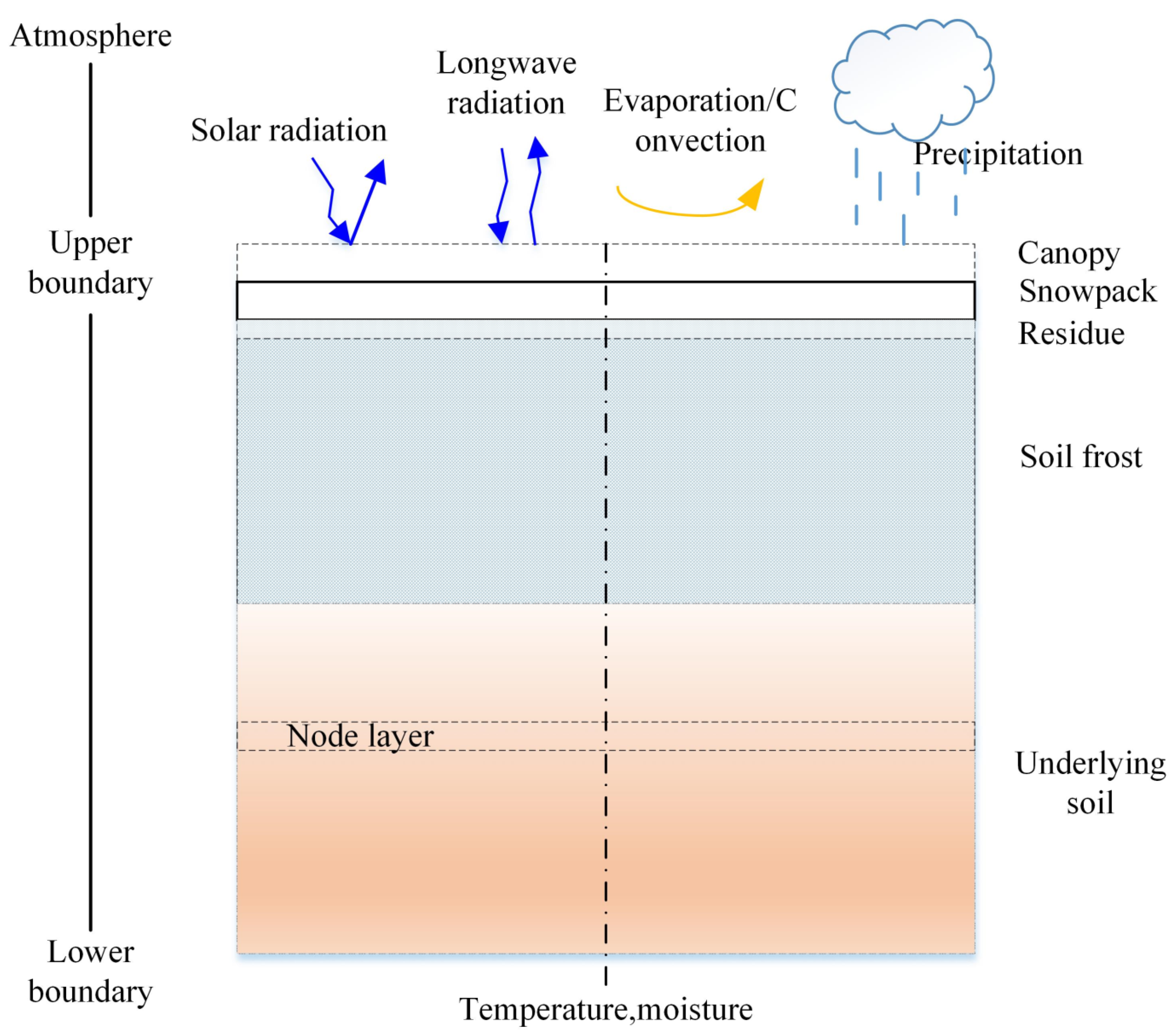
In this study, the Simultaneous Heat and Water (SHAW) model developed by Flerchinger and Saxton (1989) at the Northwest Watershed Research Center of the U.S. Department of Agriculture is chosen to simulate the hydrothermal processes in the frozen area [12]. The SHAW model version 3.0.2, whose code is available through the USDA Northwest Watershed Research Center website (https://www.ars.usda.gov/pacific-west-area/boise-id/northwest-watershed-research-center/docs/shaw-model/ (accessed on 1 August 2022)), is used for modelling. This model is a one-dimensional hydrothermal coupling model that is designed to simulate water, energy and solute transfer within a vertical profile that includes soil, vegetation cover, residue and snow. The physical system of the SHAW model is shown in Figure 3. The model differs from other models in three ways: first, it can simulate water, heat, and solute fluxes simultaneously; second, it can simulate soil freeze–thaw processes in detail; and third, it provides a method to simulate transpiration and water transfer within a multi-species plant canopy. The SHAW model provides a variety of ecohydrological information, including soil freeze–thaw, infiltration, runoff, groundwater infiltration, seedling germination and vegetation growth. In recent years, the SHAW model has been widely used in snow melt and soil freeze–thaw studies in cold regions, and the results show that the model can accurately simulate soil freezing depth and hydrothermal processes in frozen areas [13,28,29]. The SHAW model has become an important tool for the study of ecohydrological processes in cold regions.
The principles of the SHAW model can be found in the SHAW model technical paper [30]. The key processes of the SHAW model used in this study are presented as follows.
2.2.1. Energy and Water Fluxes at the Soil Surface
The energy and water input into the soil are calculated from meteorological factors, including the in situ precipitation, relative humidity, air temperature, solar radiation and wind speed observations. The energy inputs of the frozen soil are calculated by the surface energy balance equation, which is written as
where represents the net all-wave radiation, shows the sensible energy flux and is energy flux of the ground or the soil. represents the latent heat flux, among which represents latent energy of evaporation and represents the total evapotranspiration from the surface.
2.2.2. Energy Fluxes in the Soil
For a layer of frozen soil, the state equation for distribution of temperature in the soil matrix, taking into account convective heat transfer by liquid and latent energy transfer by vapor, is given by
where represents the specific heat term for change in energy stored due to a temperature rise, represents latent heat required to freeze water, is net thermal conduction into a layer, represents net thermal advection into layer due to water flux and represents net latent heat evaporation within the soil layer. and are the volumetric heat capacity and temperature of the soil, represents density of ice, represents volumetric ice content, represents soil thermal conductivity, represents density of water, represents specific heat capacity of water, represents liquid water flux, represents water vapor flux and represents vapor density within the soil.
2.2.3. Water Fluxes in the Soil
The water flux equation in the soil for freezing and thawing soil can be written as
where is the change in volumetric liquid content and is the change in volumetric ice content. In the right term of the equation, represents net liquid flux into a layer, is net vapor flux into a layer and represents the source/sink term for water extracted by roots. In addition, and represent unsaturated hydraulic conductivity and soil matric potential, respectively.
In the SHAW model, the key input values that represent vegetation conditions include LAI, dry biomass and plant albedo. In this study, the changes in these variables are considered to represent the change in vegetation conditions.
2.3. Input Data for Modelling
The SHAW model is driven by four types of in situ observation data, including the weather data, the soil temperature data, the soil moisture data and the site characteristics data. In the study, the study period is July 2020–July 2021, and hourly time step is used for modelling.
The weather data include hourly air temperature (°C), wind speed (m/s), relative humidity (%), precipitation (mm) and total solar radiation (W/m2). These weather data are acquired from the in situ automatic monitoring station (Figure 2), which is equipped with the 05103 wind speed and direction sensor (Campbell, Logan, UT, USA), the HMP155A temperature and humidity sensor (Vaisala, Vantaa, Finland), the CS106 atmospheric pressure sensor (Vaisala, Vantaa, Finland), the NR01 net radiation sensor (Hukseflux, Delft, The Netherlands) and the T-200B weighing rain and snow sensor (Geonor, Augusta, NJ, USA). Among these, the 05103 wind speed and direction sensor can observe wind speed and direction. The HMP155A temperature and humidity sensor can provide data on air temperature, air moisture and water vapor pressure. The NR01 net radiation sensor observes upward and downward long-wave and short-wave radiation.
The input soil temperature and moisture data are data observed at different buried depths from 0 to 100 cm at 10 cm intervals at the beginning of the modelling, which are used to initialize the soil profile. To improve the model performance, soil temperature and moisture data at 100 cm are used as model constraints. Observed soil temperature and moisture data of 10 to 90 cm at 10 cm intervals during the study period are used to evaluate the performance of the SHAW model. These soil data are acquired from the CS650 soil temperature/moisture sensor (Campbell, Logan, UT, USA) at the in situ station, which is equipped with probes at 10 cm burial depth intervals, ranging from 10 cm to 100 cm burial depth. The CS650 soil temperature/moisture sensor acquires the dielectric constant, soil moisture and volumetric conductivity by analyzing the original measured values of transmission time, signal attenuation and temperature. The measured signal attenuation is a correction for the loss effect and propagation time used for reflection detection. Loss effect correction allows the probe to measure high-precision volumetric moisture content in soil with a volumetric conductivity of ≤3 dS/m, without the need for specific soil calibration. A thermistor near the surface of the epoxy resin that maintains thermal contact with the probe is used to measure temperature. In the in situ station, the sensor is installed horizontally; accurate temperature measurements at the same depth as the soil moisture measurement can be obtained. The monitoring frequency of the CS650 censor in the in situ station used in the study is 10 min, which helps to solve the problem caused by strongly diurnal variability of soil temperature and moisture in cold regions. It should be mentioned that the CS650 soil moisture sensor set in the study cannot provide soil temperature and soil moisture data at the the buried depth of 0 cm; soil temperature data at the depth of 0 cm are calculated as in [31]:
where and represent the upward and downward long-wave radiation (W/m2), respectively; is the surface emissivity, set as 0.98 in the study, and is the Stefan–Boltzmann constant. Furthermore, soil moisture at a depth of 0 cm is calculated by the exponential filter based on the soil moisture observations at a depth of 10 cm. This filter assumes that the time variation at deeper soil moisture is linked to the differences between upper and deeper soil moisture [32]:
where and represent soil moisture at depth of 0 cm and the observing time point and the previous observing time , respectively, while and represent soil moisture at depth of 10 cm and the observing time point and the previous observing time , respectively. is the gain term. is the characteristic time length parameter, which is calculated by soil moisture observations at depths of 10 cm and 20 cm based on the corresponding Equations of (5) and (6).
The site characteristics data for modelling include basic site data, vegetation characteristics data, soil characteristics data, etc. In the basic site data, the noon time is set to 14, and the aerodynamic roughness is set to 0.47 cm. In the vegetation characteristics data, the plant height, leaf width, aggregation, dry biomass, LAI and rooting depth values are measured by the in situ station, and the remaining vegetation parameters are the recommended values of the SHAW model. In the soil characteristics data, the composition of soil and saturated volumetric moisture content at each buried depth are the measured data. Some researchers use in situ experimentation to acquire hydraulic parameters [33]. In the current research, the hydraulic parameters are adjusted to make the simulated value and the measured value match to the maximum extent. The Campbell equation is selected as the soil water dissipation curve. The soil characteristic parameters are shown in Table 1.
2.4. Scenario Design for Modelling
To model the influence of vegetation change on hydrothermal processes, firstly, the SHAW model is used to simulate the hydrothermal processes of the frozen soil based on observed meteorological and frozen soil data to see the performance of the SHAW model. The Nash–Sutcliffe efficiency coefficient (NSE), root mean square error (RMSE), correlation coefficient (CC) and relative error (RE) are used to evaluate the performance of the modelled soil temperature and moisture at the depths from 10 cm to 90 cm at 10 cm intervals.
The influences of vegetation changes on the hydrothermal processes of frozen soil are modelled by changing the input vegetation conditions of the model. In the SHAW model, the key input values which represent vegetation conditions include leaf area index (LAI), dry biomass and surface albedo. Generally, an increase in LAI is always accompanied by an increase in dry biomass and a decrease in surface albedo [34,35]. However, the functional relationships between the LAI, dry biomass and surface albedo are far more complex. In this study, the influences of the LAI, dry biomass and surface albedo on the soil temperature and moisture are investigated, respectively, by changing the input values from −100% to 100% at 10% intervals, and then the overlying effects of the change in LAI, dry biomass and surface albedo are discussed.
3. Results and Discussion
This section shows the observed hydrothermal processes of frozen soil and the corresponding meteorological conditions firstly, followed by the performance of the modelled hydrothermal processes of the SHAW model. The result of the modelled influence of vegetation changes on the hydrothermal processes is shown last.
3.1. Observed Hydrothermal Processes of Frozen Soil and the Corresponding Meteorological Conditions
Meteorological factors directly control the input water and energy of frozen soil. Air temperature directly affects the change of soil temperature and then affects the phase state of water in soil, while precipitation directly affects the change of soil moisture. Figure 4 shows the change trend of the soil temperature and moisture at the representative depths coupled with their directly related meteorological factors. From Figure 4a, the change trend of soil temperature at different depths is highly related to that of air temperature. This is because both the air and soil are heated by solar radiation, and the heat in the air is one of the main sources of the input or output heat of the frozen soil. The soil temperature has a significant lag phenomenon compared to the air temperature with the deepening of the burial depth. In addition, the fluctuation range of the soil temperature at the deeper burial depth is smaller than that at the shallow burial depth. This is because it takes a certain time and energy consumption in the energy transfer process between the air and deeper soil. The soil temperature is higher than the air temperature on the whole, especially at the upper layer. This is because it is easier for the soil to absorb heat from the solar radiation than the air. Furthermore, the soil heat capacity is higher than the air heat capacity; the soil can store more energy.
Comparing Figure 4a with Figure 4b, there is a correlation between soil moisture and soil temperature. When the warm season transitions to the cold season, the soil moisture decreases sharply since the soil starts to freeze after the point when the soil temperature drops to below zero, while when the cold season transitions to the warm season, the soil moisture increases rapidly since the soil starts to freeze. The lag phenomenon of the change between upper and deeper soil temperature affects the exact time when soil freezes or thaws during change of season. As seen in Figure 4b, when the cold season changes to the warm season, the precipitation gradually increases, and the soil water rapidly reaches saturation in a short time under the unfrozen state of the soil. As the precipitation is concentrated in the warm season, the upper soil moisture in the warm season keeps fluctuating around the maximum value until the precipitation decreases. It can be seen that when precipitation is high, only soil moisture at a depth of 90 cm has an obvious peak in Figure 4b, but generally, soil moisture at deeper layers has a smoother curve than that at shallower layers when the lateral flow is not considered. It can be predicted that the lateral flow may occur at deep layers in the in situ station. Furthermore, the peak value of soil moisture at the depth of 90 cm is larger than that at other layers; this may be due to the fact that the saturated volumetric moisture content is larger at this layer. In addition, after the upper soil fills with water in the warm season, the excess precipitation supplements the lower soil. Thus, the lower soil moisture is more affected by rainfall accumulation than the upper soil moisture.
3.2. Performance of Modelled Hydrothermal Processes of SHAW Model
3.2.1. Performance of Modelled Soil Temperature (ST) at Different Depths
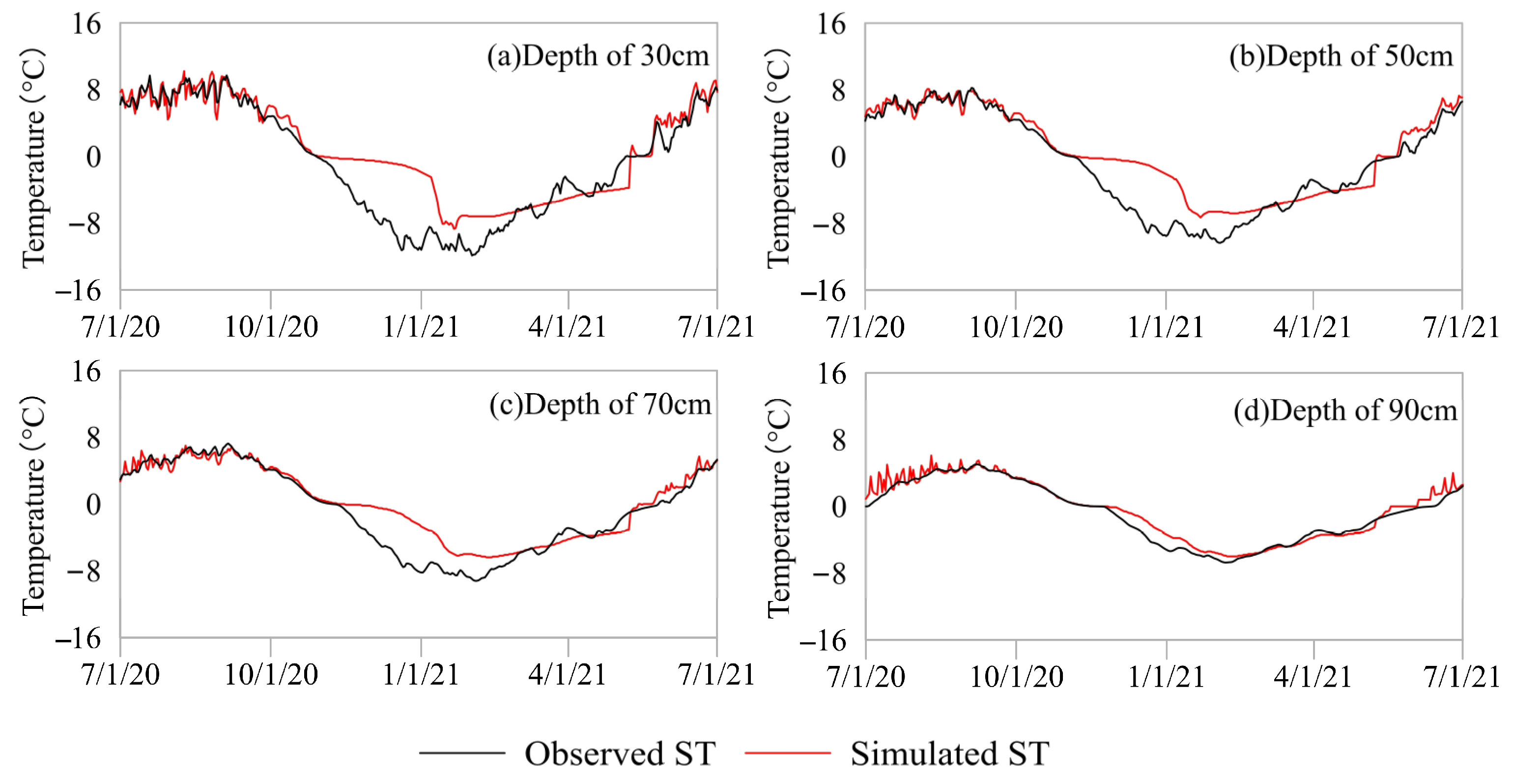
Table 2 presents the performance of modelled soil temperature (ST) of the SHAW model at different burial depths. Figure 5 shows the change trend of simulated and measured soil temperatures at representative depths. From Table 2, it can be seen that the NSE between ST simulations and ST observations is above 0.7 for all different depths, while the RMSE is basically lower than 4 °C, and the CC is above 0.88. This means that the SHAW model shows good performance in soil temperature simulation. The RE shows relatively worse performance; this is because the observed STs are around 0 °C. Although there is only a minor difference between the observed and modelled ST, the value of RE can be large. Comparing the performance of ST at different depths, the ST simulations at deeper layers show better performance than those at upper layers. The NSE, RMSE, CC and RE between ST simulations and observations at a 10 cm depth is 0.74, 3.94 °C, 0.89 and 1.66, respectively, while those at 50 cm depth are 0.8, 2.55 °C, 0.93 and 1.45, respectively. This is because the observed soil temperature data at 100 cm depth are used as the underlying interface constraints, and STs at different layers are closely related through energy transfer. Thus, the ST simulations match ST observations better when the soil layer is close to the underlying interface. From Figure 5, comparing the performance of ST at different seasons, it can be seen that the performance of ST in the warm season is better than that in the cold season. When the ST is lower than 0 °C, the ST simulations are significantly higher than the observed values, and the declining trend of the ST simulations is significantly behind the observations. This is mainly because the ST is affected by the soil heat flux, and the soil heat flux simulation is related to the net radiation value. According to relevant research, the uncertainty of net radiation simulations of the SHAW model in the cold season is larger than that in the warm season [13,36]. Furthermore, air temperature is lower than soil temperature in the cold season; it is more likely that the heat is transferred from deep soil to upper soil. Thus, the ST simulations at the upper layer in the cold season show a significant difference to the observations under a situation where the deep ST is used as a lower boundary constraint.
3.2.2. Performance of Modelled Soil Moisture (SM) at Different Depths
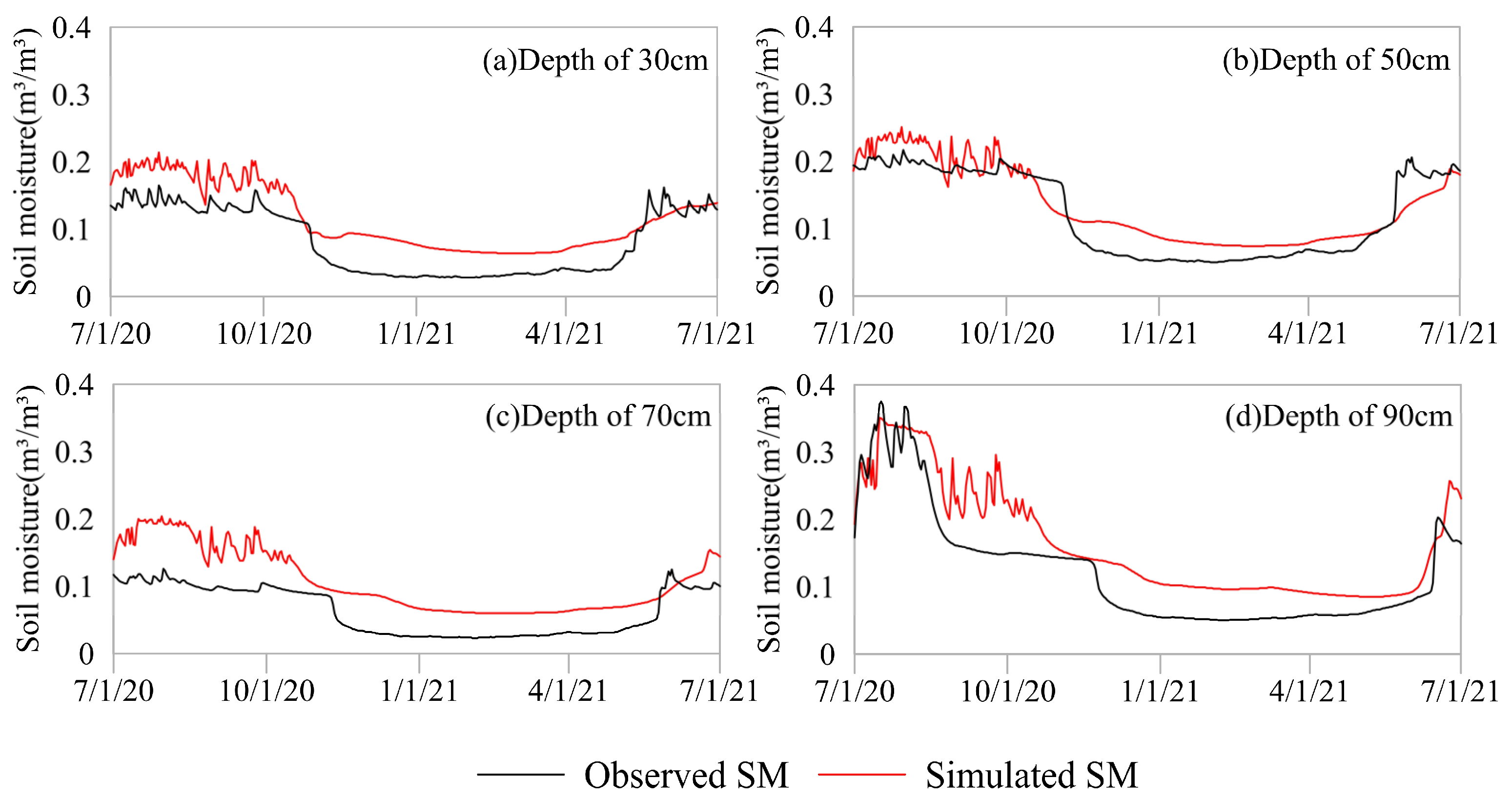
The performance of the modelled soil moisture (SM) of the SHAW model at different burial depths is presented in Table 3, and the change trends of SM simulations and observations are shown in Figure 6. From Table 3, it can be seen that the simulated values of SM in each layer of the model are basically consistent with the observed values. The correlation coefficient CC is more than 0.89 for all layers. Comparing the performance of SM simulations at different depths, the difference between the simulated and measured values of SM does not show an obvious trend of continuous decrease from the upper layer to the deep layer as in the ST simulations. The SM simulations at 40 cm depth show the best performance; the NSE reaches 0.82, while the SM simulations at 70 cm and 80 cm depths are poor, and the NSE is negative. This is because there is a high correlation of ST between layers due to the significant influence on ST from heat transfer, but the relationship of SM between layers, which is largely affected by soil characteristics and lateral and vertical flow, is much more complex. In the in situ station for modelling, since the precipitation is limited, the soil water is generally saturated from deeper layers; thus, the lateral runoff is more likely to appear at deeper layers. The SHAW model used in the study is a vertical model; it takes no consideration of complex conditions such as lateral runoff, which may lead to the poor performance of SM simulations at deeper layers. However, it can be seen that the performance of SM simulations at a depth of 90 cm is not bad; where the NSE reaches 0.65, this is because this layer is quite close to the lower boundary at depth of 100 cm, where the observed SM values are used as modelling constraints. It does not mean that there is no lateral flow at the depths of 90 cm and 100 cm.
Comparing the performance of SM in different seasons, the simulated values of SM in the warm season fluctuate in a small range, while in the cold season, the change is relatively flat. This is because sufficient precipitation in the warm season leads to a situation where the soil water is basically saturated; the SM fluctuates with the precipitation in a small range. From Figure 4, it can be seen that the SM simulations are higher than the SM observations in both the warm season and cold season. Considering the abundant precipitation in the warm season, the lateral flow which the SHAW model does not take into account may be the reason for the higher simulated values of SM in the warm season. In addition, the higher simulated values of SM in the cold season may be due to the low measured value caused by soil freezing. When the warm and cold seasons alternate, the simulated values of SM change more slowly than the measured values from the upper layer to the deeper layer. Comparing SM simulations at different depths, it can be seen that the change nodes of simulated values of SM in each layer are consistent with the change nodes of soil moisture in the upper layer, which is significantly ahead of the observed values. Thus, the simulated value of ST decreases more slowly than the measured value at this stage, resulting in the slow freezing of SM at deeper layers.
3.3. Modelled Influence of Vegetation Changes on the Hydrothermal Processes
3.3.1. Modelled Influence of Vegetation Changes on the Soil Temperature (ST) at Representative Depths
The averaged change rates of soil temperature (ST) at representative depths when the LAI, dry biomass and surface albedo change are shown in Figure 7. It can be seen that the influence of the LAI on ST simulations is more significant than that of the dry biomass and the surface albedo. The changes of dry biomass show no influence on the ST simulations, and those of surface albedo show only little influence on the ST simulations of the SHAW model, indicating that the dry biomass and surface albedo are not sensitive parameters for the ST simulations of the SHAW model. This is because the solar radiation calculation within the canopy of the SHAW model is based on the LAI values, rather than dry biomass and surface albedo values. This study chooses LAI, dry biomass and surface albedo to represent the vegetation conditions; the influence of any one of these three indexes on ST simulations represents the influence of vegetation conditions on ST. Generally speaking, the increase in LAI corresponds to the increase in dry biomass and the decrease in surface albedo; thus, although the influence of dry biomass and surface albedo on ST is not obvious in the modelling, this does not mean that the LAI is the only influential factor for ST. The LAI in this study is more like a representative of vegetation conditions.
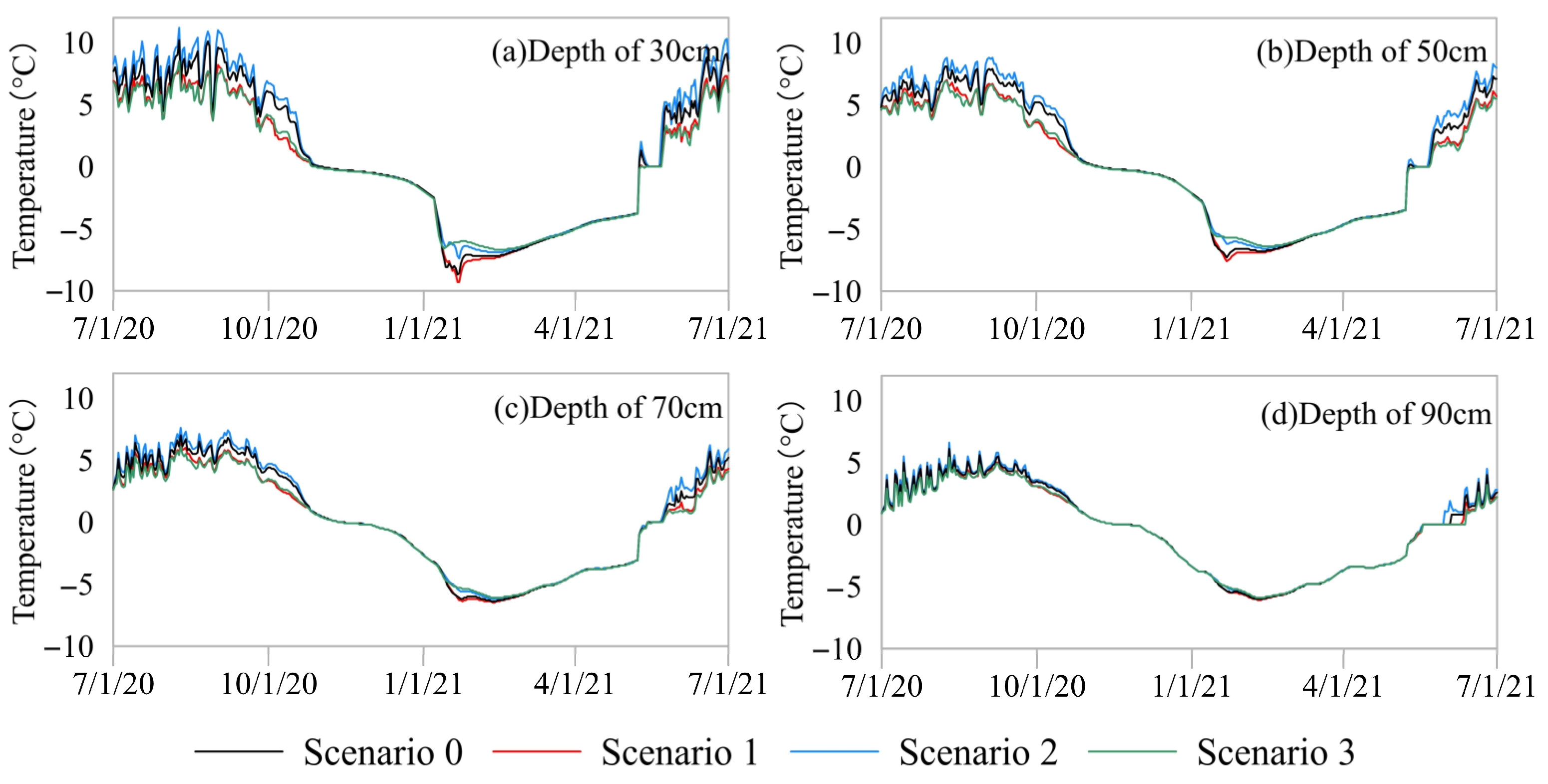
The change rate of ST shows a trend that increases firstly and then decreases when the change rate of the LAI increases from −100% to 100%. When the change rate of the LAI is −50%, the change rate of the ST reaches the top, while when the change rate of the LAI is −100% (bare soil), the change rate of the ST drops to the bottom, which is slightly lower than that when the LAI increases by 100%. This is because the bare soil loses heat quickly, and the net radiation received by the surface soil decreases when the LAI increases. Comparing the changes of ST at different depths, the change amplitude of ST becomes smaller at the deeper depth. This is because the vegetation directly affects the surface soil temperature by affecting net radiation and evapotranspiration, while there is less direct impact of vegetation on deep soil. Figure 8 presents the change trends of ST in three representative modelling scenarios, among which the LAI decrease of 100% (bare soil) and 50%, and increase of 100% are, respectively, set as scenarios 1, 2 and 3; they are compared to the original modelling scenario, which is shown as scenario 0. It can be seen that the warm season is the main growth period of vegetation and is the key period for vegetation to affect the change of soil temperature.
Overall, when the LAI decreases by lower than 60%, the ST increases for nearly all depths, and when the LAI decreases by higher than 60% or increases, the ST decreases for nearly all depths. Furthermore, the warm period is the key period when the ST simulations are affected by the vegetation changes.
3.3.2. Modelled Influence of Vegetation Changes on the Soil Moisture (SM) at Representative Depths
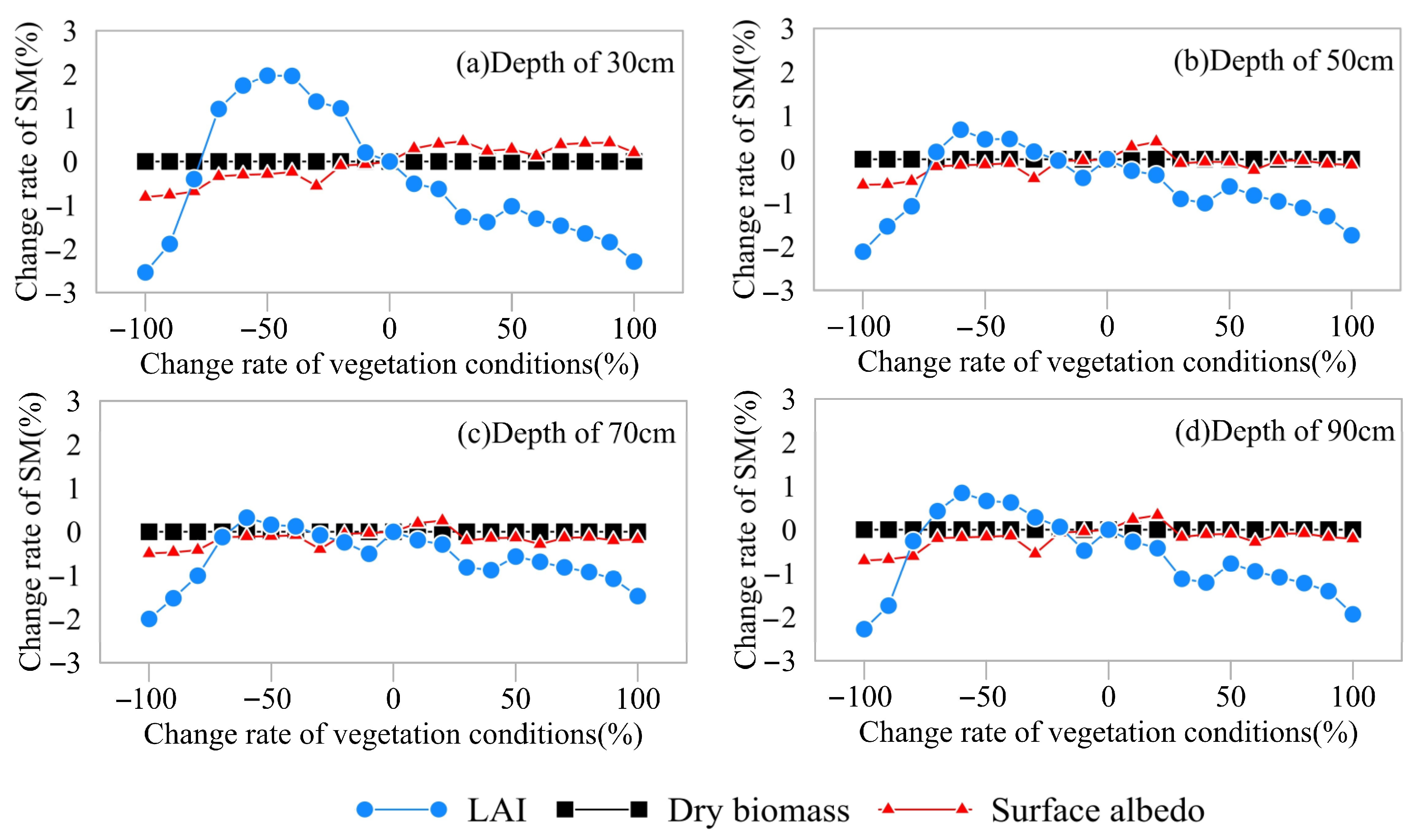
The change rate of soil moisture (SM) at representative depths when the LAI, dry biomass and surface albedo change is shown in Figure 9. It can be seen that the SM is less influenced by vegetation conditions compared to the ST. The highest change rate of ST reaches 10% when vegetation conditions change, but the change rates of SM are below 3%. From the results, the same as for ST simulations, the LAI is the main vegetation factor influencing the SM simulations of the SHAW model, and the influence of dry biomass and surface albedo can be negligible. As the change rate of LAI increases from −100% (bare soil) to 100%, the SM simulations show an increasing trend firstly, and then show a mainly declining trend after the change rate of the LAI is higher than −60% and −50%. The change trends of SM are similar to those of ST when the vegetation conditions change. It can be inferred that the vegetation conditions mainly affect the SM through changing the ST. Furthermore, the highest change rate of SM at the depth of 30 cm appears when the change rate of the LAI is −50%, and at the deeper depths, the highest values appear when the change rate is −60%. It can be noticed that the peaks of change rate of either ST or SM simulations at nearly all depths appear at around −50% change of vegetation conditions. The reason that the turning points are the same is that the vegetation changes influence SM through changing ST, and they change soil conditions at deeper layers through changing soil conditions at upper layers. Thus, the peak of change rate of ST at deeper layers corresponds to that at upper layers. Furthermore, the peak of change rate of SM corresponds to that of ST. Meanwhile, the change amplitudes of the SM simulations at the upper layers are greater than those at the deeper layers. This means there is a lag effect of the influence of the surface vegetation on the deeper soil.
The change trends of SM in three representative modelling scenarios and the original modelling scenario are shown in Figure 10, among which the original modelling is set as scenario 0, and the LAI decrease of 100% (bare soil), 50% and increase of 100% are set as scenarios 1, 2 and 3, respectively. It can be seen that the vegetation changes mainly affect soil moisture simulations in the freeze–thaw alternating period for nearly all the depths. This further indicates that vegetation affects the soil temperature firstly, and then affects the soil moisture. Overall, the SM simulations show declining trends when the LAI decreases by a large extent (larger than 60%) or increases, while they show increasing trends when the LAI decreases by a small extent (smaller than 50%). Furthermore, the freeze–thaw alternating period is the key period when the SM simulations are affected by the vegetation changes.
4. Conclusions
This study uses the vertical water and heat model, SHAW model, to simulate the water and heat process of frozen soil based on meteorological soil observation data from one in situ station in the Qinghai–Tibet Plateau from 2020 to 2021, and models the impact of vegetation on soil temperature and moisture changes at different burial depths in the frozen soil by changing vegetation condition parameters. By analyzing and discussing the modelling results, the main conclusions are as follows:
- (1)
- The soil temperature and moisture values simulated by the model for each layer of the frozen soil are basically consistent with the measured values over time; the simulated results of the hydrothermal processes are basically reliable.
- (2)
- For different soil layers, the performance of soil temperature simulations in the deep layer is better than that in the shallow layer, while the performance of soil moisture simulations has no significant trend as the depth changes. For different seasons, the performances of soil temperature and moisture simulations in warm season are better than those in cold season.
- (3)
- Among the LAI, dry biomass and surface albedo, the LAI is the main vegetation factor affecting the soil temperature and moisture simulations in the frozen soil, and the influence of dry biomass and surface albedo can be negligible.
- (4)
- When the LAI decreases by a large extent (larger than 60%) or increases, both the soil temperature and moisture show declining trends, and when the LAI decreases by a small extent (smaller than 50%), the soil temperature and moisture simulations show increasing trends.
- (5)
- The warm period is the key period when soil temperature simulations are affected by the vegetation changes, while the freeze–thaw alternating period is the key period when soil moisture simulations are affected by the vegetation changes.
This study describes possible changes in hydrothermal processes when vegetation conditions change in the Qinghai–Tibet Plateau, which can provide technical support to arrange future human activities in the frozen soil. The limitation of this research is that only one in situ station covered with low alpine meadows was used to analyze the influence of vegetation change; thus, the results are only applicable to areas of the Qinghai–Tibet Plateau that are covered by low alpine meadows. In further research, the influence of vegetation changes on hydrothermal processes can be modelled on more soil types and catchments to further validate the applicability of these results.
Author Contributions
Conceptualization, H.Y. and X.H. (Xiaofeng Hong); Data curation, X.H. (Xiaofeng Hong) and X.H. (Xiaobo He); Formal analysis, H.Y.; Funding acquisition, Z.Y.; Investigation, H.Y. and X.H. (Xiaofeng Hong); Methodology, H.Y.; Resources, X.H. (Xiaofeng Hong) and X.H. (Xiaobo He); Supervision, X.H. (Xiaofeng Hong); Validation, H.Y. and Z.Y.; Visualization, H.Y.; Writing—original draft, H.Y.; Writing—review and editing, Z.Y. All authors have read and agreed to the published version of the manuscript.
Funding
This research was funded by the National Key Research and Development Program, grant number 2022YFC3201704, and National Natural Science Foundation of China, grant number 52209007, and Major Science and Technology Projects of the Ministry of Water Resources in 2022, grant number SKS-2022039, and Central Public-Interest Scientific Institution Basal Research Fund, grant number CKSF2021485/SZ.
Data Availability Statement
Restrictions apply to the availability of these data. Data were obtained from the Field Scientific Observation and Research Station of the Water Ecosystem in the Yangtze River Source Region of the Ministry of Water Resources, and Tanggula Cryosphere and Environment Observation and Research Station of the Northwest Research Institute of the Chinese Academy of Sciences.
Acknowledgments
The authors are grateful for the ground station data support provided by the Field Scientific Observation and Research Station of the Water Ecosystem in the Yangtze River Source Region of the Ministry of Water Resources, and the Tanggula Cryosphere and Environment Observation and Research Station of the Northwest Research Institute of the Chinese Academy of Sciences.
Conflicts of Interest
The authors declare no conflict of interest.
References
- Wang, S.; Jin, H.; Li, S.; Lin, Z. Permafrost degradation on the Qinghai–Tibet Plateau and its environmental impacts. Permafr. Periglac. Process. 2000, 11, 43–53. [Google Scholar] [CrossRef]
- Immerzeel, W.W.; van Beek, L.P.H.; Bierkens, M.F.P. Climate change will affectthe Asian water towers. Science 2010, 328, 1382–1385. [Google Scholar] [CrossRef] [PubMed]
- Cuo, L.; Zhang, Y.; Bohn, T.J.; Zhao, L.; Li, J.; Liu, Q.; Zhou, B. Frozen soil degradation and its effects on surface hydrology in the northern Tibetan Plateau. J. Geophys. Res. Atmos. 2015, 120, 8276–8298. [Google Scholar] [CrossRef] [Green Version]
- Li, D.; Cui, B.; Wang, Y.; Xiao, B.; Jiang, B. Glacier extent changes and possible causes in the Hala Lake Basin of Qinghai-Tibet Plateau. J. Mt. Sci. 2019, 16, 1571–1583. [Google Scholar] [CrossRef]
- Shi, R.; Yang, H.; Yang, D. Spatiotemporal variations in frozen ground and their impacts on hydrological components in the source region of the Yangtze river. J. Hydrol. 2020, 590, 125237. [Google Scholar] [CrossRef]
- Williams, P.J.; Smith, M.W. The Frozen Earth; Cambridge University Press: Cambridge, UK, 1989. [Google Scholar]
- Gruber, S. Derivation and analysis of a high-resolution estimate of global permafrost zonation. Cryosphere 2012, 6, 221–233. [Google Scholar] [CrossRef] [Green Version]
- Wang, Y.; Yang, H.; Bing, G.; Wang, T.; Yue, Q.; Yang, D. Frozen ground degradation may reduce future runoff in the headwaters of an inland river on the northeastern Tibetan plateau. J. Hydrol. 2018, 564, 1153–1164. [Google Scholar] [CrossRef]
- Zhang, W.; An, S.; Xu, Z.; Cui, J.; Xu, Q. The impact of vegetation and soil on runoff regulation in headwater streams on the east Qinghai-Tibet Plateau, China. CATENA 2011, 87, 182–189. [Google Scholar] [CrossRef]
- Xue, X.; Xu, M.; You, Q.; Peng, F. Influence of experimental warming on heat and water fluxes of alpine meadows in the Qinghai-Tibet Plateau. Arct. Antarct. Alp. Res. 2014, 46, 441–458. [Google Scholar] [CrossRef] [Green Version]
- Yu, Z.; Wang, G.; Wang, Y. Response of biomass spatial pattern of alpine vegetation to climate change in permafrost region of the Qinghai-Tibet Plateau, China. J. Mt. Sci. 2010, 7, 301–314. [Google Scholar] [CrossRef]
- Flerchinger, G.N.; Saxton, K.E. Simultaneous heat and water model of a freezing snow-residue-soil system I. Theory and development. Trans. ASAE 1989, 32, 565–571. [Google Scholar] [CrossRef]
- He, H.; Flerchinger, G.N.; Kojima, Y.; He, D.; Hardegree, S.P.; Dyck, M.F.; Horton, R.; Lv, J.; Wang, J. Evaluation of 14 frozen soil thermal conductivity models with observations and SHAW model simulations. Geoderma 2021, 403, 115207. [Google Scholar] [CrossRef]
- Jansson, P.E.; Moon, D.S. A coupled model of water, heat and mass transfer using object orientation to improve flexibility and functionality. Environ. Model. Softw. 2001, 16, 37–46. [Google Scholar] [CrossRef]
- Zhang, W.; Wang, G.X.; Zhou, J.; Liu, G.S.; Wang, Y.B. Simulating the water-heat processes in permafrost regions in the Tibetan Plateau based on CoupModel. J. Glaciol. Geocryol. 2012, 34, 1099–1109. (In Chinese) [Google Scholar]
- Wu, M.; Zhao, Q.; Jansson, P.E.; Wu, J.; Zhang, W. Improved soil hydrological modeling with the implementation of salt-induced freezing point depression in CoupModel: Model calibration and validation. J. Hydrol. 2021, 596, 125693. [Google Scholar] [CrossRef]
- Li, Y.; Wan, Z.; Sun, L. Simulation of carbon exchange from a permafrost peatland in the Great Hing’an Mountains based on CoupModel. Atmosphere 2022, 13, 44. [Google Scholar] [CrossRef]
- Arnold, J.G.; Fohrer, N. SWAT2000: Current capabilities and research opportunities in applied watershed modeling. Hydrol. Process. 2005, 19, 563–572. [Google Scholar] [CrossRef]
- Pomeroy, J.W.; Gray, D.M.; Brown, T.; Hedstrom, N.R.; Quinton, W.L.; Granger, R.J.; Carey, S.K. The cold regions hydrological model: A plant form for basing process representation and model structure on physical evidence. Hydrol. Process. 2007, 21, 2650–2667. [Google Scholar] [CrossRef]
- Zhou, J.; Pomeroy, J.W.; Zhang, W.; Cheng, G.; Wang, G.; Chen, C. Simulating cold regions hydrological processes using a modular model in the west of China. J. Hydrol. 2014, 509, 13–24. [Google Scholar] [CrossRef] [Green Version]
- Francesconi, W.; Srinivasan, R.; Perez-Minana, E.; Willcock, S.P.; Quintero, M. Using the Soil and Water Assessment Tool (SWAT) to model ecosystem services: A systematic review. J. Hydrol. 2016, 535, 625–636. [Google Scholar] [CrossRef]
- Diao, C.; Liu, Y.; Zhao, L.; Zhuo, G.; Zhang, Y. Regional-scale vegetation-climate interactions on the Qinghai-Tibet Plateau. Ecol. Inform. 2021, 65, 101413. [Google Scholar] [CrossRef]
- Ma, S.; Yang, B.; Zhao, J.; Tan, C.; Chen, J.; Mei, Q.; Hou, X. Hydrothermal dynamics of seasonally frozen soil with different vegetation coverage in the Tianshan Mountains. Front. Earth Sci. 2022, 9, 806309. [Google Scholar] [CrossRef]
- Zhao, A.; Wang, D.; Xiang, K.; Zhang, A. Vegetation photosynthesis changes and response to water constraints in the Yangtze River and Yellow River Basin, China. Ecol. Indic. 2022, 143, 109331. [Google Scholar] [CrossRef]
- Zhang, J.; Zhang, Y.; Sun, G.; Song, C.; Li, J.; Hao, L.; Liu, N. Climate variability masked greening effects on water yield in the Yangtze River Basin during 2001–2018. Water Resour. Res. 2022, 58, e2021WR030382. [Google Scholar] [CrossRef]
- Li, H.; Liu, G.; Fu, B. Response of vegetation to climate change and human activity based on NDVI in the Three-River Headwaters region. Acta Ecol. Sin. 2011, 31, 5495–5504, (In Chinese with English abstract). [Google Scholar] [CrossRef]
- Chang, F.; Qin, Z.; Cheng, W.; He, X. Analysis on the temperature and moisture of frozen soil in the typical watershed of Yangtze River Source area and its influencing factors. J. China Hydrol. 2021, 41, 62–68. (In Chinese) [Google Scholar] [CrossRef]
- Li, R.; Shi, H.; Flerchinger, G.N.; Akae, T.; Wang, C. Simulation of freezing and thawing soils in Inner Mongolia Hetao Irrigation District, China. Geoderma 2012, 173–174, 28–33. [Google Scholar] [CrossRef]
- Liu, B.; Shao, M. Modeling soil-water dynamics and soil-water carrying capacity for vegetation on the Loess Plateau, China. Agric. Water Manag. 2015, 159, 176–184. [Google Scholar] [CrossRef]
- Flerchinger, G.N. The Simultaneous Heat and Water (SHAW) Model: Technical Documentation; Technical Report NWRC 2017-02; Northwest Watershed Research Center, USDA Agricultural Research Service: Boise, ID, USA, 2017.
- Yang, K.; Wang, J. A temperature prediction-correction method for estimating surface soil heat flux from soil temperature and moisture data. Sci. Chine Ser. D Earth Sci. 2008, 51, 721–729. [Google Scholar] [CrossRef]
- Wagner, W.; Lemoine, G.; Rott, H. A method for estimating soil moisture from ERS scatterometer and soil data. Remote Sens. Environ. 1999, 70, 191–207. [Google Scholar] [CrossRef]
- Batsilas, I.; Angelaki, A.; Chalkidis, I. Hydrodynamics of the Vadose Zone of a Layered Soil Column. Water 2023, 15, 221. [Google Scholar] [CrossRef]
- Ning, Z.; Yoon, J. Expansion of the world’s deserts due to vegetation-albedo feedback under global warming. Geophys. Res. Lett. 2009, 36, L17401. [Google Scholar] [CrossRef] [Green Version]
- Loranty, M.M.; Berner, L.T.; Goetz, S.J.; Jin, Y.; Randerson, J.T. Vegetation controls on northern high latitude snow-albedo feedback: Observations and CMIP5 model simulations. Glob. Change Biol. 2014, 20, 594–606. [Google Scholar] [CrossRef]
- Zhen, L.; Gan, Y.; Wei, J.; Li, R.; Wu, Y.; Wang, G. Numerical simulation of coupled process of freeze-thaw soil water and heat in alpine regions based on SHAW model. Water Resour. Hydropower Eng. 2022, 53, 194–204. (In Chinese) [Google Scholar] [CrossRef]
Figure 1.
The influential factors of hydrothermal processes.

Figure 2.
The location of the in situ station in the Tanggula frozen area (a) and China (b), and the vegetation condition of the in situ station (c).
Figure 2.
The location of the in situ station in the Tanggula frozen area (a) and China (b), and the vegetation condition of the in situ station (c).

Figure 3.
Physical system of SHAW model.

Figure 4.
The change trend of (a) air temperature (AT) and soil temperature (ST), (b) precipitation (P) and soil moisture (SM) at representative depths, among which, ST30, ST50, ST70 and ST90 represent soil temperature at 30 cm, 50 cm, 70 cm and 90 cm depths, and SM30, SM50, SM70 and SM90 represent soil moisture at 30 cm, 50 cm, 70 cm and 90 cm depths.

Figure 5.
Comparison of observed and simulated soil temperature (ST) at representative depths.

Figure 6.
Comparison of observed and simulated soil moisture (SM) at representative depths.

Figure 7.
The averaged change rate of soil temperature (ST) at representative depths with variation of vegetation conditions.
Figure 7.
The averaged change rate of soil temperature (ST) at representative depths with variation of vegetation conditions.

Figure 8.
The change trends of soil temperature (ST) at representative depths in three representative modelling scenarios (scenario 1, 2, 3) and the original modelling scenario (scenario 0).
Figure 8.
The change trends of soil temperature (ST) at representative depths in three representative modelling scenarios (scenario 1, 2, 3) and the original modelling scenario (scenario 0).

Figure 9.
The averaged change rate of soil moisture (SM) at representative depths with variation of vegetation conditions.
Figure 9.
The averaged change rate of soil moisture (SM) at representative depths with variation of vegetation conditions.

Figure 10.
The change trends of soil moisture (SM) at representative depths in three representative modelling scenarios (scenario 1, 2, 3) and the original modelling scenario (scenario 0).
Figure 10.
The change trends of soil moisture (SM) at representative depths in three representative modelling scenarios (scenario 1, 2, 3) and the original modelling scenario (scenario 0).


Table 1.
Soil characteristic parameters of SHAW model at different depths.
| Depth (cm) | Percent of Soil Composition (%) | Bulk Density (kg/m3) | Saturated Volumetric Moisture Content (m3/m3) | ||||
|---|---|---|---|---|---|---|---|
| Sand | Silt | Clay | Error | Measured Values | Error | ||
| 0 | 65 | 25 | 10 | 5 | 1176 | 0.259 | 0.05 |
| 10 | 69 | 21 | 10 | 5 | 1235 | 0.259 | 0.05 |
| 20 | 67 | 23 | 10 | 5 | 1203 | 0.218 | 0.05 |
| 30 | 55 | 35 | 10 | 5 | 1100 | 0.246 | 0.05 |
| 40 | 56 | 30 | 14 | 5 | 1100 | 0.209 | 0.05 |
| 50 | 57 | 30 | 13 | 5 | 1100 | 0.286 | 0.05 |
| 60 | 57 | 30 | 13 | 5 | 1100 | 0.237 | 0.05 |
| 70 | 57 | 30 | 13 | 5 | 1100 | 0.23 | 0.05 |
| 80 | 60 | 30 | 10 | 5 | 1125 | 0.304 | 0.05 |
| 90 | 60 | 30 | 10 | 5 | 1125 | 0.375 | 0.05 |
| 100 | 47 | 43 | 10 | 5 | 1090 | 0.411 | 0.05 |
Table 2.
The performance of simulated soil temperature (ST) at different depths.
| Depths (cm) | 10 | 20 | 30 | 40 | 50 | 60 | 70 | 80 | 90 |
|---|---|---|---|---|---|---|---|---|---|
| NSE | 0.74 | 0.75 | 0.77 | 0.78 | 0.8 | 0.83 | 0.85 | 0.89 | 0.94 |
| RMSE (°C) | 3.94 | 3.61 | 3.22 | 2.91 | 2.55 | 2.19 | 1.98 | 1.42 | 0.84 |
| CC | 0.89 | 0.9 | 0.91 | 0.92 | 0.93 | 0.94 | 0.94 | 0.96 | 0.98 |
| RE | 1.66 | 1.62 | 1.60 | 1.56 | 1.45 | 1.28 | 1.07 | 0.83 | 0.48 |
Table 3.
The performance of simulated soil moisture (SM) at different depths.
| Depths (cm) | 10 | 20 | 30 | 40 | 50 | 60 | 70 | 80 | 90 |
|---|---|---|---|---|---|---|---|---|---|
| NSE | 0.77 | 0.63 | 0.34 | 0.82 | 0.79 | 0.46 | −0.84 | −0.23 | 0.65 |
| RMSE (m3/m3) | 0.03 | 0.03 | 0.04 | 0.02 | 0.03 | 0.03 | 0.05 | 0.06 | 0.05 |
| CC | 0.9 | 0.89 | 0.91 | 0.92 | 0.91 | 0.9 | 0.89 | 0.90 | 0.93 |
| RE | −0.07 | −0.25 | −0.42 | −0.05 | −0.11 | −0.32 | −0.69 | −0.62 | −0.32 |
Disclaimer/Publisher’s Note: The statements, opinions and data contained in all publications are solely those of the individual author(s) and contributor(s) and not of MDPI and/or the editor(s). MDPI and/or the editor(s) disclaim responsibility for any injury to people or property resulting from any ideas, methods, instructions or products referred to in the content. |
© 2023 by the authors. Licensee MDPI, Basel, Switzerland. This article is an open access article distributed under the terms and conditions of the Creative Commons Attribution (CC BY) license (https://creativecommons.org/licenses/by/4.0/).
Share and Cite
MDPI and ACS Style
Yang, H.; Hong, X.; Yuan, Z.; He, X. Modelling the Influence of Vegetation on the Hydrothermal Processes of Frozen Soil in the Qinghai–Tibet Plateau. Water 2023, 15, 1692. https://doi.org/10.3390/w15091692
AMA Style
Yang H, Hong X, Yuan Z, He X. Modelling the Influence of Vegetation on the Hydrothermal Processes of Frozen Soil in the Qinghai–Tibet Plateau. Water. 2023; 15(9):1692. https://doi.org/10.3390/w15091692
Chicago/Turabian StyleYang, Han, Xiaofeng Hong, Zhe Yuan, and Xiaobo He. 2023. "Modelling the Influence of Vegetation on the Hydrothermal Processes of Frozen Soil in the Qinghai–Tibet Plateau" Water 15, no. 9: 1692. https://doi.org/10.3390/w15091692
Note that from the first issue of 2016, this journal uses article numbers instead of page numbers. See further details here.