

Seasonal Streamflow Forecast in the Tocantins River Basin, Brazil: An Evaluation of ECMWF-SEAS5 with Multiple Conceptual Hydrological Models
 , , ,
, , ,
Abstract
:1. Introduction
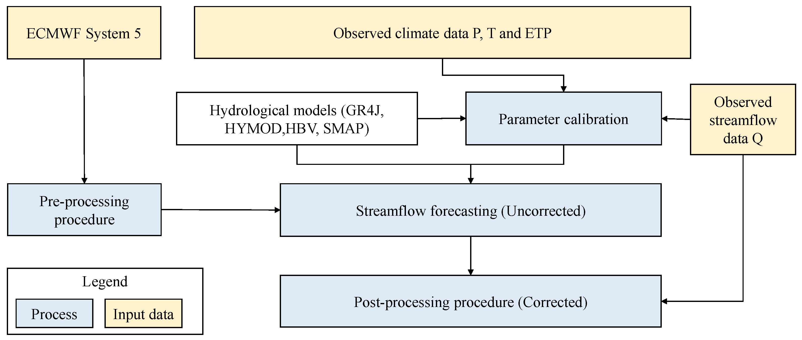
2. Methodology
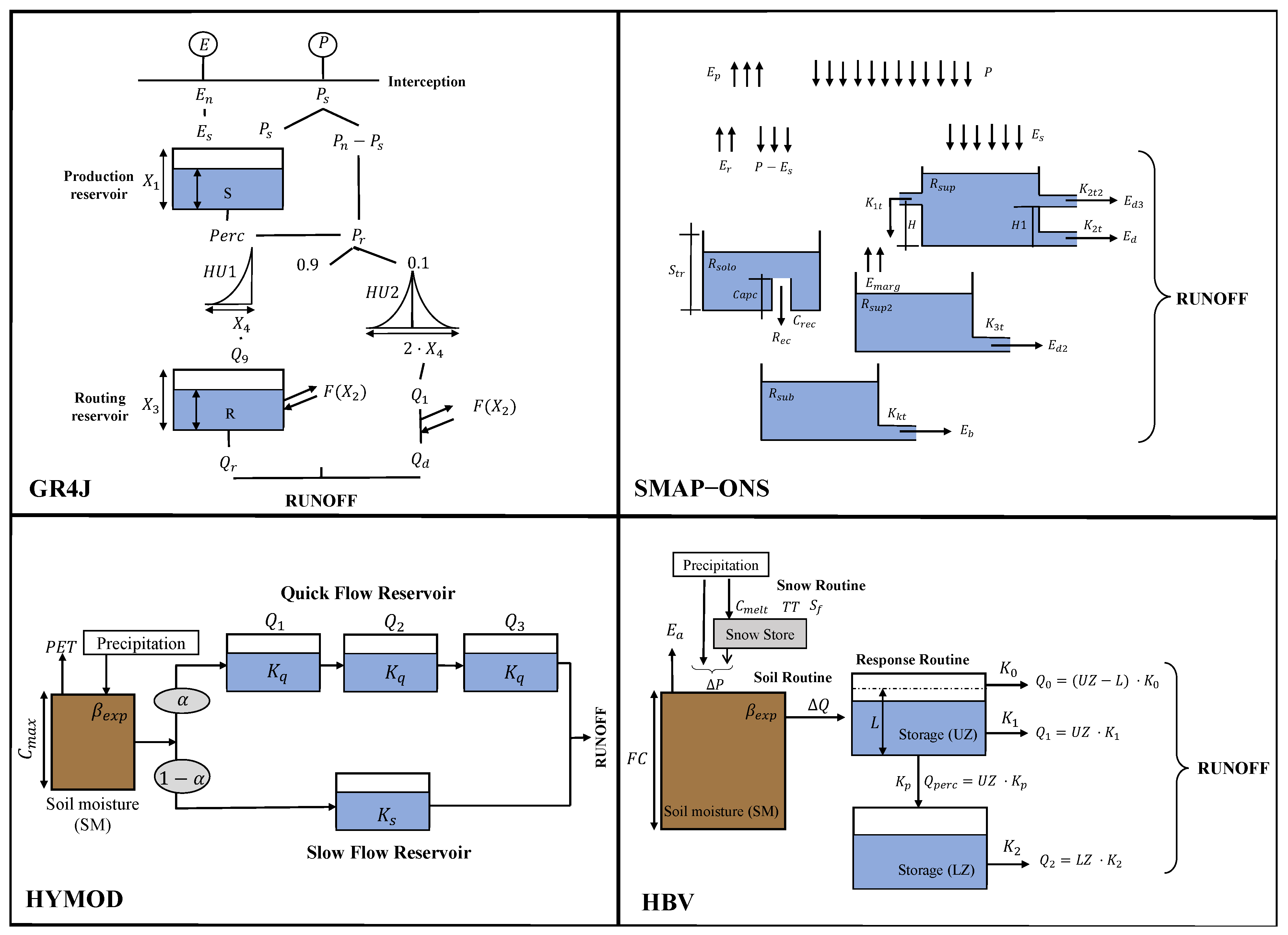
2.1. Hydrological Models
2.1.1. HYMOD Model
2.1.2. GR4J Model
2.1.3. SMAP Model
2.1.4. HBV Model
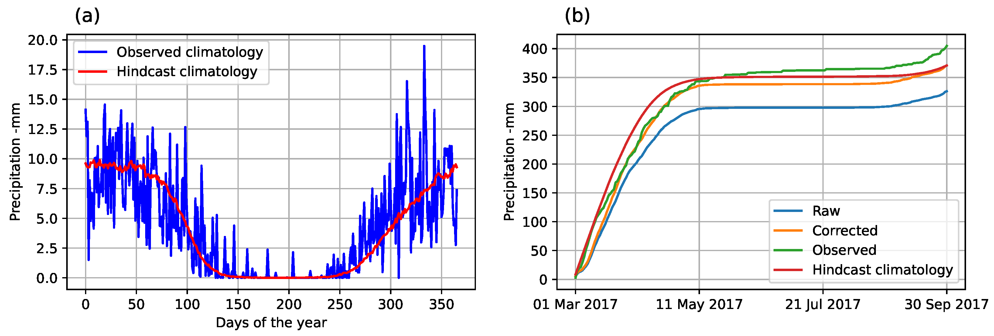
2.2. ECMWF-SEAS5 Data
2.3. Post-Processing Procedure
2.4. Performance Metrics
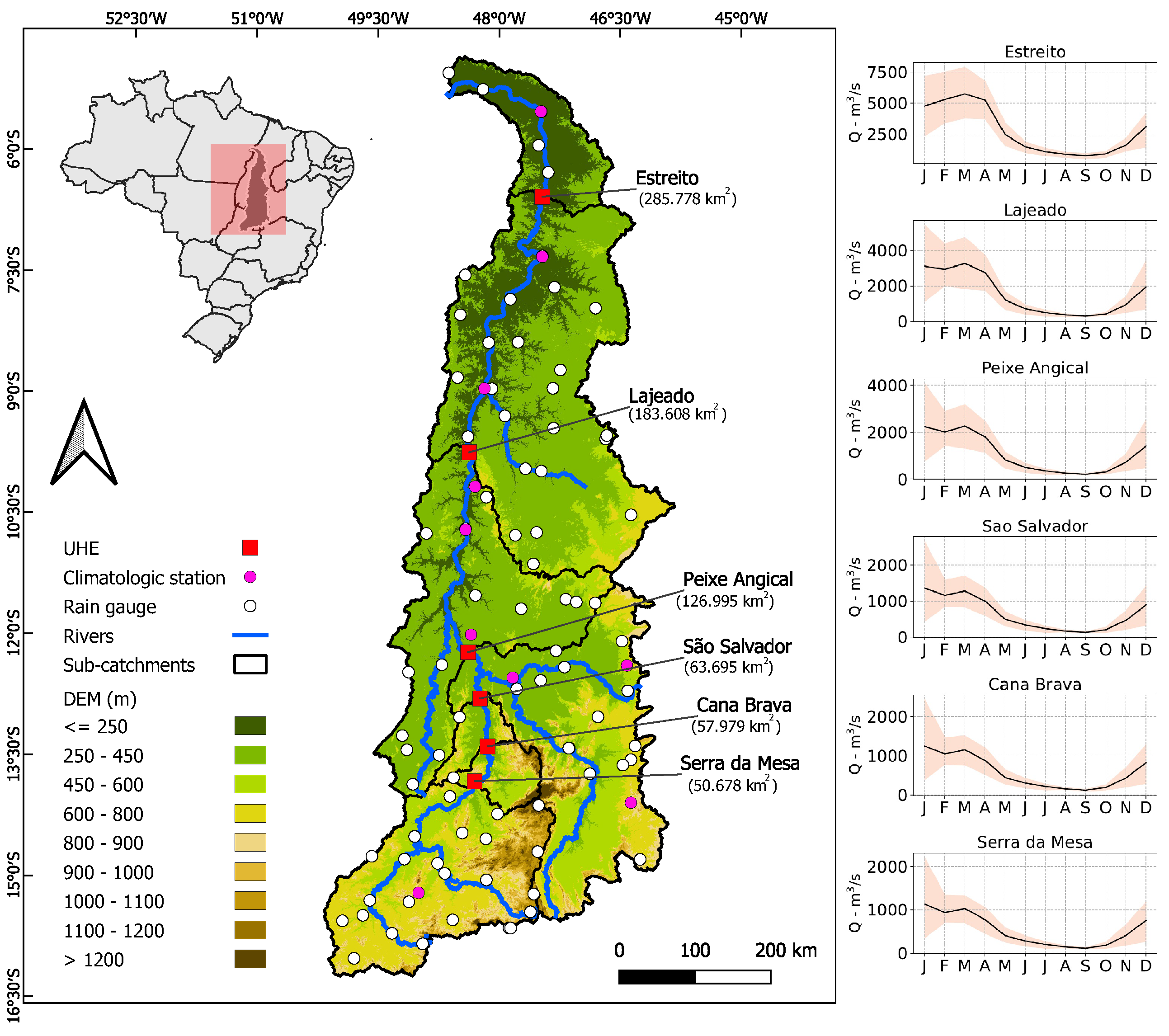
3. Case Study
3.1. Overview and Data
3.2. Results Analysis
4. Conclusions
Author Contributions
Funding
Data Availability Statement
Acknowledgments
Conflicts of Interest
References
- Maurer, E.P.; Lettenmaier, D.P. Potential effects of long-lead hydrologic predictability on Missouri River main-stem reservoirs. J. Clim. 2004, 17, 174–186. [Google Scholar] [CrossRef]
- Tian, F.; Li, Y.; Zhao, T.; Hu, H.; Pappenberger, F.; Jiang, Y.; Lu, H. Evaluation of the ECMWF System 4 climate forecasts for streamflow forecasting in the Upper Hanjiang River Basin. Hydrol. Res. 2018, 49, 1864–1879. [Google Scholar] [CrossRef]
- Graham, N.E.; Georgakakos, K.P. Toward understanding the value of climate information for multiobjective reservoir management under present and future climate and demand scenarios. J. Appl. Meteorol. Climatol. 2010, 49, 557–573. [Google Scholar] [CrossRef]
- Xu, W.; Zhang, C.; Peng, Y.; Fu, G.; Zhou, H. A two stage B ayesian stochastic optimization model for cascaded hydropower systems considering varying uncertainty of flow forecasts. Water Resour. Res. 2014, 50, 9267–9286. [Google Scholar] [CrossRef]
- Ávila, L.; Mine, M.R.; Kaviski, E. Probabilistic long-term reservoir operation employing copulas and implicit stochastic optimization. Stoch. Environ. Res. Risk Assess. 2020, 34, 931–947. [Google Scholar] [CrossRef]
- Li, H.; Liu, P.; Guo, S.; Ming, B.; Cheng, L.; Yang, Z. Long-term complementary operation of a large-scale hydro-photovoltaic hybrid power plant using explicit stochastic optimization. Appl. Energy 2019, 238, 863–875. [Google Scholar] [CrossRef]
- DelSole, T. Predictability and information theory. Part I: Measures of predictability. J. Atmos. Sci. 2004, 61, 2425–2440. [Google Scholar] [CrossRef]
- Bazile, R.; Boucher, M.A.; Perreault, L.; Leconte, R. Verification of ECMWF System 4 for seasonal hydrological forecasting in a northern climate. Hydrol. Earth Syst. Sci. 2017, 21, 5747–5762. [Google Scholar] [CrossRef]
- Cheng, M.; Fang, F.; Kinouchi, T.; Navon, I.; Pain, C. Long lead-time daily and monthly streamflow forecasting using machine learning methods. J. Hydrol. 2020, 590, 125376. [Google Scholar] [CrossRef]
- Tyralis, H.; Papacharalampous, G.; Langousis, A. Super ensemble learning for daily streamflow forecasting: Large-scale demonstration and comparison with multiple machine learning algorithms. Neural Comput. Appl. 2021, 33, 3053–3068. [Google Scholar] [CrossRef]
- Kisi, O.; Cimen, M. A wavelet-support vector machine conjunction model for monthly streamflow forecasting. J. Hydrol. 2011, 399, 132–140. [Google Scholar] [CrossRef]
- Zhang, H.; Yang, Q.; Shao, J.; Wang, G. Dynamic streamflow simulation via online gradient-boosted regression tree. J. Hydrol. Eng. 2019, 24, 04019041. [Google Scholar] [CrossRef]
- Solomatine, D.P.; Ostfeld, A. Data-driven modelling: Some past experiences and new approaches. J. Hydroinform. 2008, 10, 3–22. [Google Scholar] [CrossRef]
- Zhao, T.; Schepen, A.; Wang, Q. Ensemble forecasting of sub-seasonal to seasonal streamflow by a Bayesian joint probability modelling approach. J. Hydrol. 2016, 541, 839–849. [Google Scholar] [CrossRef]
- Hadi, S.J.; Tombul, M. Monthly streamflow forecasting using continuous wavelet and multi-gene genetic programming combination. J. Hydrol. 2018, 561, 674–687. [Google Scholar] [CrossRef]
- Day, G.N. Extended streamflow forecasting using NWSRFS. J. Water Resour. Plan. Manag. 1985, 111, 157–170. [Google Scholar] [CrossRef]
- Faber, B.A.; Stedinger, J. Reservoir optimization using sampling SDP with ensemble streamflow prediction (ESP) forecasts. J. Hydrol. 2001, 249, 113–133. [Google Scholar] [CrossRef]
- Sabzipour, B.; Arsenault, R.; Brissette, F. Evaluation of the potential of using subsets of historical climatological data for ensemble streamflow prediction (ESP) forecasting. J. Hydrol. 2021, 595, 125656. [Google Scholar] [CrossRef]
- Harrigan, S.; Prudhomme, C.; Parry, S.; Smith, K.; Tanguy, M. Benchmarking ensemble streamflow prediction skill in the UK. Hydrol. Earth Syst. Sci. 2018, 22, 2023–2039. [Google Scholar] [CrossRef]
- Fan, F.M.; Collischonn, W.; Quiroz, K.; Sorribas, M.; Buarque, D.; Siqueira, V. Flood forecasting on the Tocantins River using ensemble rainfall forecasts and real-time satellite rainfall estimates. J. Flood Risk Manag. 2016, 9, 278–288. [Google Scholar] [CrossRef]
- Keteklahijani, V.K.; Alimohammadi, S.; Fattahi, E. Predicting changes in monthly streamflow to Karaj dam reservoir, Iran, in climate change condition and assessing its uncertainty. Ain Shams Eng. J. 2019, 10, 669–679. [Google Scholar] [CrossRef]
- Johnson, S.J.; Stockdale, T.N.; Ferranti, L.; Balmaseda, M.A.; Molteni, F.; Magnusson, L.; Tietsche, S.; Decremer, D.; Weisheimer, A.; Balsamo, G.; et al. SEAS5: The new ECMWF seasonal forecast system. Geosci. Model Dev. 2019, 12, 1087–1117. [Google Scholar] [CrossRef]
- Ferreira, G.W.; Reboita, M.S.; Drumond, A. Evaluation of ECMWF-SEAS5 Seasonal Temperature and Precipitation Predictions over South America. Climate 2022, 10, 128. [Google Scholar] [CrossRef]
- Darbandsari, P.; Coulibaly, P. Inter-comparison of lumped hydrological models in data-scarce watersheds using different precipitation forcing data sets: Case study of Northern Ontario, Canada. J. Hydrol. Reg. Stud. 2020, 31, 100730. [Google Scholar] [CrossRef]
- Yang, D.; Herath, S.; Musiake, K. Comparison of different distributed hydrological models for characterization of catchment spatial variability. Hydrol. Process. 2000, 14, 403–416. [Google Scholar] [CrossRef]
- Staudinger, M.; Stahl, K.; Seibert, J.; Clark, M.; Tallaksen, L. Comparison of hydrological model structures based on recession and low flow simulations. Hydrol. Earth Syst. Sci. 2011, 15, 3447–3459. [Google Scholar] [CrossRef]
- Ghimire, U.; Agarwal, A.; Shrestha, N.K.; Daggupati, P.; Srinivasan, G.; Than, H.H. Applicability of lumped hydrological models in a data-constrained river basin of Asia. J. Hydrol. Eng. 2020, 25, 05020018. [Google Scholar] [CrossRef]
- Jiang, T.; Chen, Y.D.; Xu, C.y.; Chen, X.; Chen, X.; Singh, V.P. Comparison of hydrological impacts of climate change simulated by six hydrological models in the Dongjiang Basin, South China. J. Hydrol. 2007, 336, 316–333. [Google Scholar] [CrossRef]
- Jaiswal, R.; Ali, S.; Bharti, B. Comparative evaluation of conceptual and physical rainfall–runoff models. Appl. Water Sci. 2020, 10, 48. [Google Scholar] [CrossRef]
- Ávila, L.; Silveira, R.; Campos, A.; Rogiski, N.; Gonçalves, J.; Scortegagna, A.; Freita, C.; Aver, C.; Fan, F. Comparative Evaluation of Five Hydrological Models in a Large-Scale and Tropical River Basin. Water 2022, 14, 3013. [Google Scholar] [CrossRef]
- Woldemeskel, F.; McInerney, D.; Lerat, J.; Thyer, M.; Kavetski, D.; Shin, D.; Tuteja, N.; Kuczera, G. Evaluating post-processing approaches for monthly and seasonal streamflow forecasts. Hydrol. Earth Syst. Sci. 2018, 22, 6257–6278. [Google Scholar] [CrossRef]
- Naeini, M.R.; Analui, B.; Gupta, H.; Duan, Q.; Sorooshian, S. Three decades of the Shuffled Complex Evolution (SCE-UA) optimization algorithm: Review and applications. Sci. Iran. 2019, 26, 2015–2031. [Google Scholar]
- Boyle, D.P. Multicriteria Calibration of Hydrologic Models. Ph.D. Thesis, The University of Arizona, Tucson, AZ, USA, 2001. [Google Scholar]
- Perrin, C.; Michel, C.; Andréassian, V. Improvement of a parsimonious model for streamflow simulation. J. Hydrol. 2003, 279, 275–289. [Google Scholar] [CrossRef]
- Grouillet, B.; Ruelland, D.; Vaittinada Ayar, P.; Vrac, M. Sensitivity analysis of runoff modeling to statistical downscaling models in the western Mediterranean. Hydrol. Earth Syst. Sci. 2016, 20, 1031–1047. [Google Scholar] [CrossRef]
- Tian, Y.; Xu, Y.P.; Zhang, X.J. Assessment of climate change impacts on river high flows through comparative use of GR4J, HBV and Xinanjiang models. Water Resour. Manag. 2013, 27, 2871–2888. [Google Scholar] [CrossRef]
- Traore, V.B.; Sambou, S.; Tamba, S.; Fall, S.; Diaw, A.T.; Cisse, M.T. Calibrating the rainfall-runoff model GR4J and GR2M on the Koulountou river basin, a tributary of the Gambia river. Am. J. Environ. Prot. 2014, 3, 36–44. [Google Scholar] [CrossRef]
- Hublart, P.; Ruelland, D.; García De Cortázar Atauri, I.; Ibacache, A. Reliability of a conceptual hydrological model in a semi-arid Andean catchment facing water-use changes. In Proceedings of the International Association of Hydrological Sciences, Koblenz, Germany, 13–16 October2015; Volume 371, pp. 203–209. [Google Scholar]
- Lopes, J.E.G.; Braga Jr, B.; Conejo, J. SMAP–A simplified hydrologic model. In Applied Modeling in Catchment Hydrology; Singh, V.P., Ed.; Water Resources Publications: Littleton, CO, USA, 1982. [Google Scholar]
- Operador Nacional do Sistema Elétrico. Amplicação do Modelo SMAP/ONS Para Previsão de vazõEs no âmbito do SIN; ONS 0097/2018-RV3; Operador Nacional do Sistema Elétrico: Rio de Janeiro, Brazil, 2018.
- Cavalcante, M.R.G.; da Cunha Luz Barcellos, P.; Cataldi, M. Flash flood in the mountainous region of Rio de Janeiro state (Brazil) in 2011: Part I—Calibration watershed through hydrological SMAP model. Nat. Hazards 2020, 102, 1117–1134. [Google Scholar] [CrossRef]
- da Cunha Luz Barcellos, P.; Cataldi, M. Flash flood and extreme rainfall forecast through one-way coupling of WRF-SMAP models: Natural hazards in Rio de Janeiro state. Atmosphere 2020, 11, 834. [Google Scholar] [CrossRef]
- Maciel, G.M.; Cabral, V.A.; Marcato, A.L.M.; Júnior, I.C.S.; Honório, L.D.M. Daily Water Flow Forecasting via Coupling Between SMAP and Deep Learning. IEEE Access 2020, 8, 204660–204675. [Google Scholar] [CrossRef]
- Singh, V.P. (Ed.) Computer Models of Watershed Hydrology; Water Res. Publ.: Highlands Ranch, CO, USA, 1992; pp. 443–476. [Google Scholar]
- Aghakouchak, A.; Habib, E. Application of a conceptual hydrologic model in teaching hydrologic processes. Int. J. Eng. Educ. 2010, 26, 963–973. [Google Scholar]
- Andréasson, J.; Bergström, S.; Carlsson, B.; Graham, L.P.; Lindström, G. Hydrological change–climate change impact simulations for Sweden. AMBIO J. Hum. Environ. 2004, 33, 228–234. [Google Scholar] [CrossRef]
- Teutschbein, C.; Seibert, J. Bias correction of regional climate model simulations for hydrological climate-change impact studies: Review and evaluation of different methods. J. Hydrol. 2012, 456, 12–29. [Google Scholar] [CrossRef]
- Nash, J.E.; Sutcliffe, J.V. River flow forecasting through conceptual models part I—A discussion of principles. J. Hydrol. 1970, 10, 282–290. [Google Scholar] [CrossRef]
- Gupta, H.V.; Sorooshian, S.; Yapo, P.O. Status of automatic calibration for hydrologic models: Comparison with multilevel expert calibration. J. Hydrol. Eng. 1999, 4, 135–143. [Google Scholar] [CrossRef]
- Hersbach, H. Decomposition of the continuous ranked probability score for ensemble prediction systems. Weather. Forecast. 2000, 15, 559–570. [Google Scholar] [CrossRef]
- Trambauer, P.; Werner, M.; Winsemius, H.; Maskey, S.; Dutra, E.; Uhlenbrook, S. Hydrological drought forecasting and skill assessment for the Limpopo River basin, southern Africa. Hydrol. Earth Syst. Sci. 2015, 19, 1695–1711. [Google Scholar] [CrossRef]
- Fawcett, T. An introduction to ROC analysis. Pattern Recognit. Lett. 2006, 27, 861–874. [Google Scholar] [CrossRef]
- Agência Nacional de Águas. Plano Estratégico de Recursos Hídricos da Bacia Hidrográfica dos Rios Tocantins e Araguaia: Relatório e síntese; Agência Nacional de Águas: Brasília, Brazil, 2009; p. 256.
- Fan, F.M.; Schwanenberg, D.; Collischonn, W.; Weerts, A. Verification of inflow into hydropower reservoirs using ensemble forecasts of the TIGGE database for large scale basins in Brazil. J. Hydrol. Reg. Stud. 2015, 4, 196–227. [Google Scholar] [CrossRef]
- Alvares, C.A.; Stape, J.L.; Sentelhas, P.C.; Gonçalves, J.D.M.; Sparovek, G. Köppen’s climate classification map for Brazil. Meteorol. Z. 2013, 22, 711–728. [Google Scholar] [CrossRef]
- Junqueira, R.; Viola, M.R.; de Mello, C.R.; Vieira-Filho, M.; Alves, M.V.; Amorim, J.D.S. Drought severity indexes for the Tocantins River Basin, Brazil. Theor. Appl. Climatol. 2020, 141, 465–481. [Google Scholar] [CrossRef]
- McNaughton, K.; Jarvis, P. Using the Penman-Monteith equation predictively. Agric. Water Manag. 1984, 8, 263–278. [Google Scholar] [CrossRef]
- Belotti, J.; Mendes, J.J.; Leme, M.; Trojan, F.; Stevan, S.L.; Siqueira, H. Comparative study of forecasting approaches in monthly streamflow series from Brazilian hydroelectric plants using Extreme Learning Machines and Box & Jenkins models. J. Hydrol. Hydromech. 2021, 69, 180–195. [Google Scholar]
- Lima, C.H.; Lall, U. Climate informed monthly streamflow forecasts for the Brazilian hydropower network using a periodic ridge regression model. J. Hydrol. 2010, 380, 438–449. [Google Scholar] [CrossRef]
- Crochemore, L.; Ramos, M.H.; Pappenberger, F.; Perrin, C. Seasonal streamflow forecasting by conditioning climatology with precipitation indices. Hydrol. Earth Syst. Sci. 2017, 21, 1573–1591. [Google Scholar] [CrossRef]


| Model Feature | GR4J | HYMOD | HBV | SMAP |
|---|---|---|---|---|
| Parameters | 4 | 5 | 11 | 11 |
| Input data | P; PET | P; PET | P; T; LMT; LMPET | P; PET |
| Conceptual storage | Production soil storage | Soil moisture layer | Soil moisture layer | Upper soil reservoir |
| Routing soil storage | Quick flow reservoirs | Upper-zone storage | Second upper-soil reservoir | |
| Slow flow reservoir | Lower-zone storage | Lower soil reservoir | ||
| Ground storage | ||||
| Type of flows | Fast flow | Surface flow | Surface flow | Surface flow |
| Slow flow | Ground water flow | Base flow | Base flow |
| Forecasted Outcome | Observed Outcome | |
|---|---|---|
| True | False | |
| True | True positive (A) | False positive (B) |
| False | False negative (C) | True negative (D) |
Disclaimer/Publisher’s Note: The statements, opinions and data contained in all publications are solely those of the individual author(s) and contributor(s) and not of MDPI and/or the editor(s). MDPI and/or the editor(s) disclaim responsibility for any injury to people or property resulting from any ideas, methods, instructions or products referred to in the content. |
© 2023 by the authors. Licensee MDPI, Basel, Switzerland. This article is an open access article distributed under the terms and conditions of the Creative Commons Attribution (CC BY) license (https://creativecommons.org/licenses/by/4.0/).
Share and Cite
Ávila, L.; Silveira, R.; Campos, A.; Rogiski, N.; Freitas, C.; Aver, C.; Fan, F. Seasonal Streamflow Forecast in the Tocantins River Basin, Brazil: An Evaluation of ECMWF-SEAS5 with Multiple Conceptual Hydrological Models. Water 2023, 15, 1695. https://doi.org/10.3390/w15091695
Ávila L, Silveira R, Campos A, Rogiski N, Freitas C, Aver C, Fan F. Seasonal Streamflow Forecast in the Tocantins River Basin, Brazil: An Evaluation of ECMWF-SEAS5 with Multiple Conceptual Hydrological Models. Water. 2023; 15(9):1695. https://doi.org/10.3390/w15091695
Chicago/Turabian StyleÁvila, Leandro, Reinaldo Silveira, André Campos, Nathalli Rogiski, Camila Freitas, Cássia Aver, and Fernando Fan. 2023. "Seasonal Streamflow Forecast in the Tocantins River Basin, Brazil: An Evaluation of ECMWF-SEAS5 with Multiple Conceptual Hydrological Models" Water 15, no. 9: 1695. https://doi.org/10.3390/w15091695