Effects of Climate Change on Streamflow in the Godavari Basin Simulated Using a Conceptual Model including CMIP6 Dataset

Abstract

Hydrological reaction to climate change anticipates water cycle alterations. To ensure long-term water availability and accessibility, it is essential to develop sustainable water management strategies and better hydrological models that can simulate peak flow. These efforts will aid in water resource planning, management, and climate change mitigation. This study develops and compares Sacramento, Australian Water Balance Model (AWBM), TANK, and SIMHYD conceptual models to simulate daily streamflow at Rajegaon station of the Pranhita subbasin in the Godavari basin of India. The study uses daily Indian Meteorological Department (IMD) gridded rainfall and temperature datasets. For 1987–2019, 70% of the models were calibrated and 30% validated. Pearson correlation (CC), Nash Sutcliffe efficiency (NSE), Root mean square error (RMSE), and coefficient of determination (CD) between the observed and simulated streamflow to evaluate model efficacy. The best conceptual (Sacramento) model selected to forecast future streamflow for the SSP126, SSP245, SSP370, and SSP585 scenarios for the near (2021–2040), middle (2041–2070), and far future (2071–2100) using EC-Earth3 data was resampled and bias-corrected using distribution mapping. In the far future, the SSP585 scenario had the most significant relative rainfall change (55.02%) and absolute rise in the annual mean temperature (3.29 °C). In the middle and far future, the 95th percentile of monthly streamflow in the wettest July is anticipated to rise 40.09% to 127.06% and 73.90% to 215.13%. SSP370 and SSP585 scenarios predicted the largest streamflow increases in all three time periods. In the near, middle, and far future, the SSP585 scenario projects yearly relative streamflow changes of 72.49%, 93.80%, and 150.76%. Overall, the findings emphasize the importance of considering the potential impacts of future scenarios on water resources to develop effective and sustainable water management practices.

1. Introduction

Climate change is the long-term, progressive alteration of local weather patterns and temperature. Global temperatures have increased as a result, which has caused sea levels to rise, oceans to warm and become more acidic, and more extreme weather patterns [1,2]. As temperatures increase, climate extremes are anticipated to become more frequent and severe, according to Pendergrass et al. [3], Wehner [4], and the Intergovernmental Panel on Climate Change (IPCC 2021) (Allan et al. [5]). The IPCC’s Sixth Assessment Report (AR6) states that climate change disproportionately affects local societies with low adaptation capacities, notably developing nations with rapidly growing populations and underdeveloped social and economic organizations (IPCC, 2022) [6]. Low-prepared communities face higher uncertainty in weather and climate systems [7].

Access to precise climate data is imperative for communities to adapt to evolving climate conditions and formulate effective strategies for adaptation and mitigation. Global circulation models (GCMs) are valuable for accumulating broad spatial and temporal records. GCMs provide information about the climate system that cannot be gained from observational data alone [8]. The World Climate Research Program (WCRP) of CMIP6 was utilized to source the GCMs used to construct climate scenario projections. Previous CMIP5 climate change forecasts under the Representative Concentration Pathway (RCP) and future socioeconomic development trajectories are incorporated into CMIP6 [9]. The shared socioeconomic paths (SSPs) represent alternative development paths for future societies in light of climate change and climate change policy. SSP1 envisions a growing push toward sustainable practices, while SSP5 assumes a socioeconomic trajectory primarily dependent on fossil fuels for energy. Both SSP1 and SSP5 exhibit generally positive human development trends, including substantial financial investments in areas such as education and healthcare, robust economic expansion, and well-functioning institutions [10]. For additional information on SSPs, please access O’Neill et al. [9]. The most recent generation of GCMs, known as CMIP6, gives a more accurate depiction of Earth’s physical phenomena than previous generations. These models use SSPs to estimate future occurrences, considering changes in the economy, technology, land use, and other environmental variables [11]. CMIP6’s coordinated trials focus on bias reduction, resulting in more accurate predictions than past models [12,13].

Climate change is expected to affect hydrological conditions and water resources at regional and global scales, resulting in changes to rainfall events, evapotranspiration, water yield, and surface runoff [14,15]. Such changes could lead to either a decrease or increase in the trend-line, with some regions experiencing water shortages and others experiencing excess water [16,17]. Droughts and floods seriously threaten agriculture and other sectors, especially in developing nations where rain-fed agriculture is a significant contributor to the economy [18]. Several studies indicate climate change will severely impact global water resources, necessitating adaptation strategies. A comprehensive comprehension of regional climate change projections and their impact on water resources is imperative in order to formulate efficacious adaptation strategies. The utilization of rainfall-runoff models in conjunction with regional climate change scenarios is a common approach for evaluating the potential effects of climate change on catchment areas. The aforementioned studies necessitate precise prognostications of future climate and reliable hydrological models that can endure evolving climate circumstances [19,20,21]. The classification of hydrological models encompasses several types, including but not limited to empirical or Blackbox models, physically-based models, and conceptual or gray-box models [22]. Conceptual models rely on empirical connections among diverse hydrological parameters and utilize primary equations to estimate meteorological inputs and basin hydrological mechanisms [23,24,25]. Achieving satisfactory outcomes with these models necessitates the calibration of data and estimation of parameters [26].

The TANK model, developed by Sugawara, is an example of a conceptual model that explains water flow concepts in a drainage basin [27,28]. Hydrologic modelers often prefer lumped models due to their simplicity, satisfactory results, and minimal data requirements, particularly when resources are scarce [29,30]. Studies have compared the performance of various models, such as TANK, AWBM, and Soil & Water Assessment Too (SWAT), for different regions in India, with TANK models being found to perform better [31,32]. The SIMHYD model is another example of a conceptual lumped model that simulates runoff from different bases in a catchment [33,34]. The Sacramento model, first developed by Burnash et al. [35] for the US National Weather Service and California Department of Water Resources, has been widely utilized worldwide. Modifications have been made to enhance its performance, such as physically based changes introduced by [36] to account for soil freezing and thawing effects. Various optimization techniques, including shuffled complex evolution, direct search, and multi-objective particle swarm optimization, have been used to calibrate the model parameters.

Farmers and industries in India’s Godavari River basin depend on the river for irrigation and other uses [37]. However, shifting rainfall patterns lead to more extreme weather events like floods and droughts [38]. Water availability for agriculture and industry is also affected by climate change, affecting crop yields and hydropower generation [39,40]. Temperature and rainfall changes also impact the basin’s biodiversity, vital to its ecological balance [41]. This study developed and compared Sacramento, AWBM, TANK, and SIMHYD conceptual models to correctly predict the Pranhita River’s daily discharge (Rajegaon Station) in the Godavari Basin, India. IMD gridded rainfall and temperature data were used to create the models, with potential evapotranspiration (PET) calculated using the Hargreaves method. The best-performing model was selected and used to project future streamflow for the study area under distinct CMIP6 scenarios (SSP126, SSP245, SSP370, and SSP585) for the near, middle, and far future based on evaluation metrics like NSE, CD, CC, and RMSE. This work is the first to use conceptual models and CMIP6 scenarios to extensively study future streamflow in the Godavari Basin. The study also suggests choosing the most accurate and efficient model, which could reduce model runtime and resource use without compromising accuracy. Sustainable water management methods that can adapt to changing conditions and reduce the region’s vulnerability to climate change are needed to mitigate climate change. This study’s conceptual model predictions of future streamflow under various CMIP6 scenarios help planners and decision-makers manage water resources and reduce flood risk. This study’s monthly, seasonal, and annual streamflow forecasts can help create sustainable water management practices that can adapt to climate change. The article’s parts are organized by structure: The authors describe the study’s topic and suggested models in “Materials and Methods”. The “results” and “discussion” sections follow, where the authors compare the models’ success indicators. The paper concludes with “conclusions” and suggestions for future research.

2. Materials and Methods

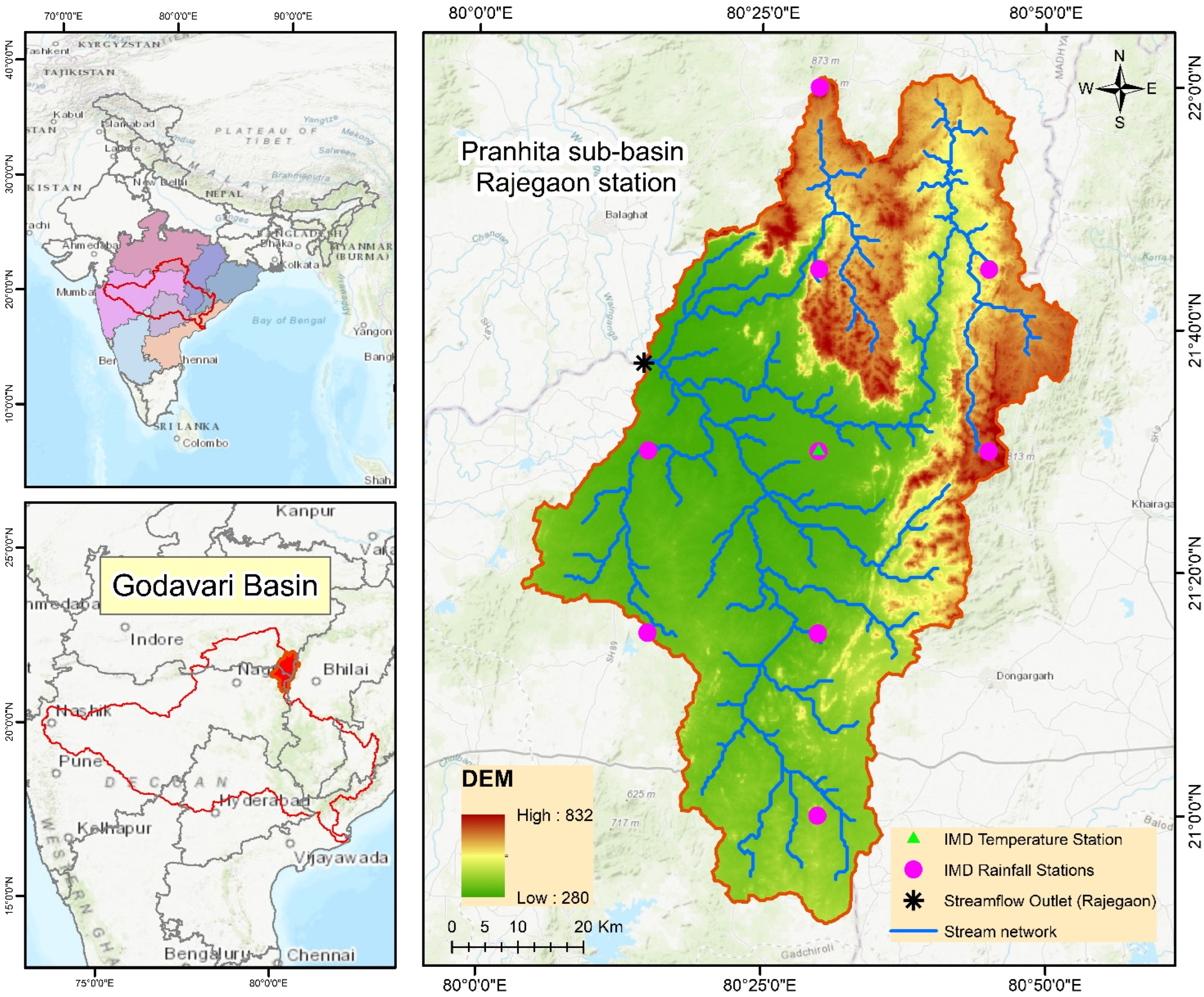
2.1. Study Area

The study area is located in the state of Madhya Pradesh, Maharashtra, and Chhattisgarh in India. The site is identified as Rajegaon with a drainage area of 5380 km². Along the Godavari River, the study region is part of the basin. The Godavari River’s Pranhita tributary flows into Wainganga. The study area’s local river is the Bagh. Nagpur’s Upper Wainganga SD is the study area’s division and sub-division. The streamflow outlet geographic location is at a latitude of 21°37′32″ and a longitude of 80°15′14″ in the Balaghat district. The study area experiences an annual rainfall range between 756.59 and 2208.76 mm, with an average annual rainfall of 1302.35 mm. This catchment receives over 90% of rainfall in the monsoon season (June–September) and the remaining 10% is received post-monsoon (October–December), in winter (January–February), and pre-monsoon (March–May) seasons. The maximum and minimum temperature in the study area varies between 32.68 °C and 19.65 °C. The study area’s average PET is 4.89 mm/day. According to Figure 1, the elevation of the research region varies from its highest point, which is 832 m, to its lowest position, which is 280 m, collected from SRTM DEM. The study area is characterized by 51.49% forest cover, 46.18% agricultural land, 1.2% water bodies, and 0.33% built-up land [42]. It is possible to identify different forest types within the forest cover based on vegetation characteristics. The most common forest types in the study area are deciduous broadleaf forest, deciduous needle leaf forest, and mixed forest.

2.2. Datasets Used

2.2.1. IMD Data

IMD generated gridded rainfall data established on gauge observations. It is possible to acquire IMD gridded rainfall data from 1901 to 2021, and they have a spatial resolution of 0.25° * 0.25° and gridded temperature at a resolution of 1° * 1°. This resolution was attained by utilizing Shepard’s interpolation method using data gathered from 6695 gauges [43,44]. Since 1951, around 3100 stations per day have been used to build the dataset. The reference rainfall data collection utilized in India has been extensively employed to address the biases present in the CMIP6 models.

2.2.2. CMIP6 Model Data

The EC-Earth3 model was employed in this study to project the streamflow. The Earth System Grid Federation (ESGF) archives are accessible for review at https://esgf-node.llnl.gov/search/cmip6, accessed on 31 August 2022, EC-Earth3 data were spatially remapped using bilinear interpolation to a normal IMD grid of 0.25° * 0.25° [45,46]. EC-Earth3 performed best in capturing extreme rainfall over India [47].

2.2.3. Streamflow Data

The daily streamflow data from the Rajegaon station were collected from the India Water Resources Information System portal (https://indiawris.gov.in/wris/#/ accessed on 31 August 2022), covering the period between 1987 and 2019.

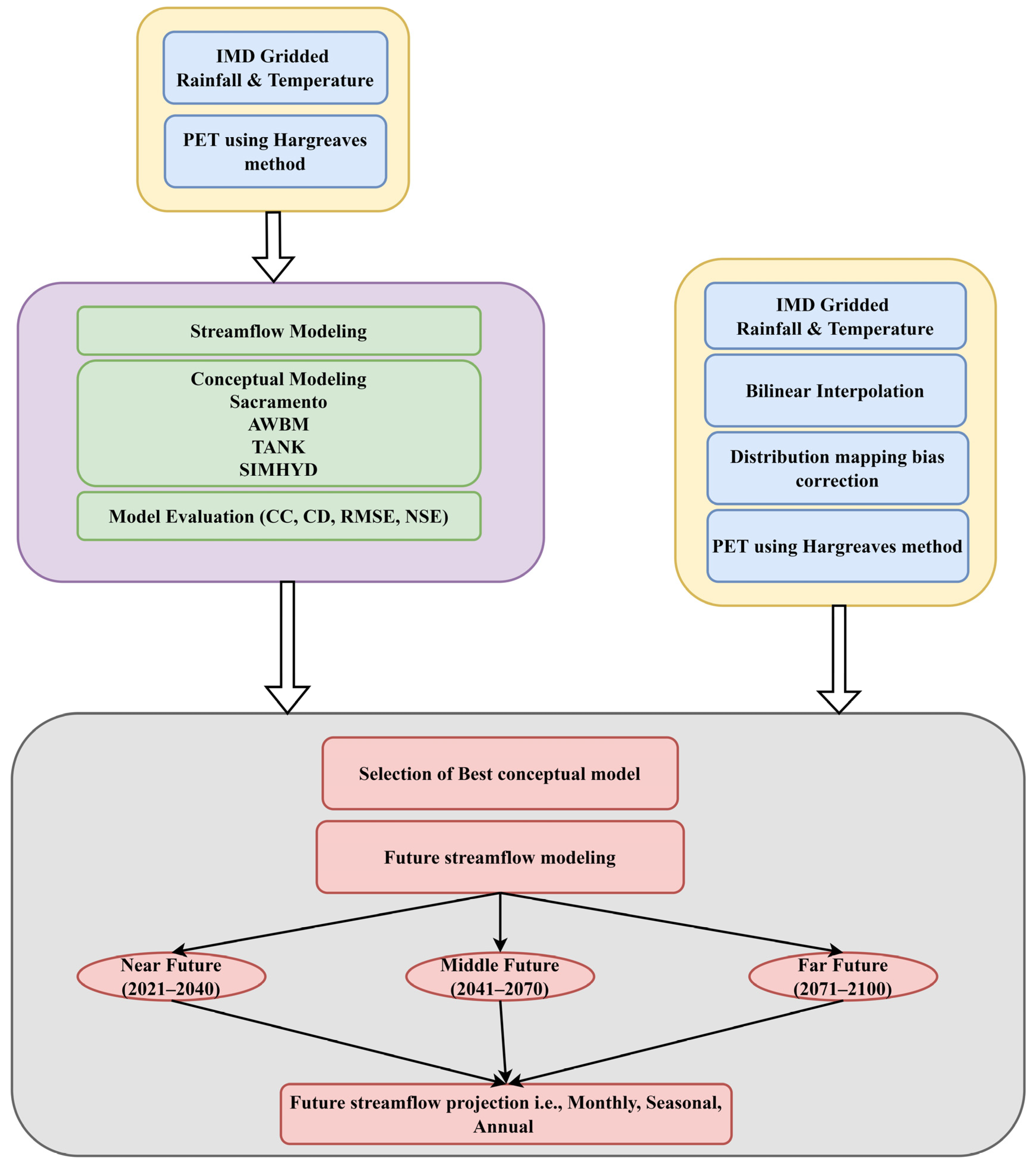
2.2.4. Data Processing

IMD Pune provided the gridded rainfall and temperature data in netCDF format, and ESGF CMIP6 data were processed and extracted using Climate Data Operators (CDO) and ArcGIS 10.3. The study area was analyzed by acquiring nine data points of gridded rainfall from IMD. The estimation of the mean rainfall was conducted through the utilization of the Thiessen polygon methodology. The EC-Earth3 dataset was bias-corrected using the Distribution mapping method, with IMD used as a reference dataset. For further information on distribution mapping, relevant literature such as Smitha et al. [48] can be accessed. Figure 2 provides a flowchart outlining the investigation’s procedures. The IMD and EC-Earth3 datasets were used to calculate PET using the Hargreaves method [49].

2.3. Conceptual Models

2.3.1. Sacramento

The Sacramento Model is a hydrological model that employs daily rainfall and PET data to estimate daily streamflow. The model emulates the hydrological equilibrium within the catchment area through the incorporation of soil moisture. In contrast to the AWBM model, the Sacramento model is characterized by a higher level of complexity, encompassing a total of five stores and twenty-two distinct attributes, as outlined in Table S1. The Sacramento model optimizes its maximum, minimum, and default values through the utilization of the genetic algorithm (GA). The hydrologically active zone of the soil in Sacramento is classified into two distinct layers, namely a relatively thin upper layer and a significantly thicker lower layer [50]. The soil moisture conditions and five runoff components are produced through the interaction of tension and free water storage areas within each layer [35,51]. The schematic representation of the Sacramento model is presented in Figure S1. The model comprises five distinct stores. The complete forms of these stores are provided in Table S1. The retention of water within the soil profile is facilitated by surface tension in tension water stores. The discharge of water from this layer is exclusively attributed to evapotranspiration. The movement of water in a free water store can occur horizontally and vertically within the soil and subsequently discharged as either baseflow (in the lower zone) or interflow (upper zone). The Sacramento model classifies the catchment into two distinct categories based on their permeability: impermeable and pervious. The impervious area is typically composed of bodies of water, such as lakes and rivers, as well as non-porous surfaces, including pavement, that are directly linked to the river network. Podger [52] thoroughly guides the Sacramento model within the RRL toolkit manual.

2.3.2. AWBM

AWBM is a theoretical framework utilized in hydrological management to evaluate rainfall losses and establish the interdependence between daily rainfall, evapotranspiration, and runoff at a watershed scale. The model comprises five distinct stores, namely three surface stores that emulate partial runoff regions, a base flow store, and a surface runoff routing store [53]. The utilization of the RRL toolkit is observed in the Pranhita subbasin for the purpose of producing daily streamflow simulations. The water balance calculation is conducted independently for every partial surface region of the AWBM, and each storage unit is allocated a distinct storage capacity [50], as illustrated in the schematic diagram depicted in Figure S2. The projections of the surface area refer to the ratios of the catchment area that depict land use or soil type as defined by the user. Table S2 outlines the parameters utilized in the AWBM model.

2.3.3. TANK

This model is both straightforward and efficient. Rainwater is collected in the topmost tank as mentioned in Figure S3. As the water level gradually decreases due to evaporation, the deficiency is compensated by drawing water from the next tank below until all tanks are emptied. The calculated runoff is then discharged from the side outlets, with the top tank output representing surface runoff, the second tank output representing intermediate runoff, the third tank output representing sub-base runoff, and the fourth tank output representing baseflow. Despite its straightforward nature, the behavior of the TANK model is complex, with the content of each tank significantly impacting the model’s performance. Notably, the same rainfall can result in significantly different runoff generation depending on the storage volumes of the tanks. The utilization of the tank model is a prevalent approach for the simulation of diurnal streamflow patterns, relying on daily inputs of rainfall and evapotranspiration, and it eliminates the need to account for the preliminary rainfall loss since its effect is already considered in the model’s nonlinear structure. The parameters used in the TANK model with default, maximum, and minimum values are mentioned in Table S3.

2.3.4. SIMHYD

Chiew et al. [33] proposed the utilization of the SIMHYD model, which employs daily rainfall and PET data to forecast the daily discharge at a designated gauging location. SIMHYD is a simplified iteration of the HYDROLOG model that was originally developed in 1972. The HYDROLOG model is a conceptual model that simulates the process of rainfall runoff. Additionally, there is another model called MODHYDROLOG [54]. SIMHYD has a comparatively smaller number of parameters, with only seven, in contrast to HYDROLOG and MODHYDROLOG, which have seventeen and nineteen parameters, respectively. The conceptual framework of SIMHYD, based on daily rainfall-runoff, is depicted in Figure S4. The SIMHYD model incorporates a mechanism whereby the daily rainfall is utilized to replenish the interception store, which is discharged daily. The surplus rainfall is subsequently subjected to an infiltration capacity assessment function. Infiltration excess runoff is the term used to describe any surplus of rainfall that surpasses the infiltration capacity. Table S4 lists the parameters utilized in the SIMHYD model and their respective default, maximum, and minimum values.

2.4. Model Performance Evaluation

At Rajegaon station, four standard evaluation metrics are examined for daily streamflow measurements, including CD, NSE, RMSE, and CC. NSE is a standardized statistic that estimates the proportion of residual variance to the variance of the actual data [44,50,55]. NSE represents the degree to which the actual streamflow and the forecasted streamflow data fit the 1:1 line. NSE ranges are mentioned in

Table 1. Model evaluation metrics.

Parameter	Expression	Range	Performance
Nash-Sutcliffe efficiency	$NSE=1-\frac{{\displaystyle \sum _{i=1}^n{(S_O^i-S_S^i)}^2}}{{\displaystyle \sum _{i=1}^n{(S_O^i-{\overline{S}}_O)}^2}}$	0.75 < NSE ≤ 1.00	Very good
		0.65 < NSE ≤ 0.75	Good
		0.50 < NSE ≤ 0.65	Satisfactory
		0.4 <NSE ≤ 0.50	Acceptable
		NSE ≤ 0.4	Unsatisfactory
Pearson correlation	$CC=\left(\frac{n{\displaystyle \sum _{i=1}^n(S_O^i}{S}_S^i)-({\displaystyle \sum _{i=1}^n{S}_O^i})({\displaystyle \sum _{i=1}^n{S}_S^i})}{\sqrt{(n{\displaystyle \sum _{i=1}^n{(S_O^i)}^2-{({\displaystyle \sum _{i=1}^n{S}_O^i})}^2)}}\sqrt{(n{\displaystyle \sum _{i=1}^n{(S_S^i)}^2-{({\displaystyle \sum _{i=1}^n{S}_S^i})}^2)}}}\right)$	−1 to 1	-
Root means square error	$RMSE=\sqrt{\frac{{\displaystyle \sum _{i=1}^n{(S_O^i-S_S^i)}^2}}{n}}$	0 to ∞	-
Coefficient of Determination	$CD={\left(\frac{n{\displaystyle \sum _{i=1}^n(S_O^i}{S}_S^i)-({\displaystyle \sum _{i=1}^n{S}_O^i})({\displaystyle \sum _{i=1}^n{S}_S^i})}{\sqrt{(n{\displaystyle \sum _{i=1}^n{(S_O^i)}^2-{({\displaystyle \sum _{i=1}^n{S}_O^i})}^2)}}\sqrt{(n{\displaystyle \sum _{i=1}^n{(S_S^i)}^2-{({\displaystyle \sum _{i=1}^n{S}_S^i})}^2)}}}\right)}^2$	0.7 < CD ≤ 0.1	Very good
		0.6 < CD ≤ 0.7	Good
		0.5 < CD ≤ 0.6	Satisfactory
		0 < CD ≤ 0.5	Unsatisfactory

with the formula [56]. CC quantifies how closely simulated data match observation data. RMSE is a frequently employed statistic for determining the difference between the values predicted by a product and the actual values. CD represents the variability of observed data. Table 1 denotes the expressions, range [56], and performance value for evaluation metrics, where $S_O^i$ represents observed streamflow data $S_S^i$ represents simulated streamflow and ${\overline{S}}_O$ represents the mean of observed streamflow data.

3. Results

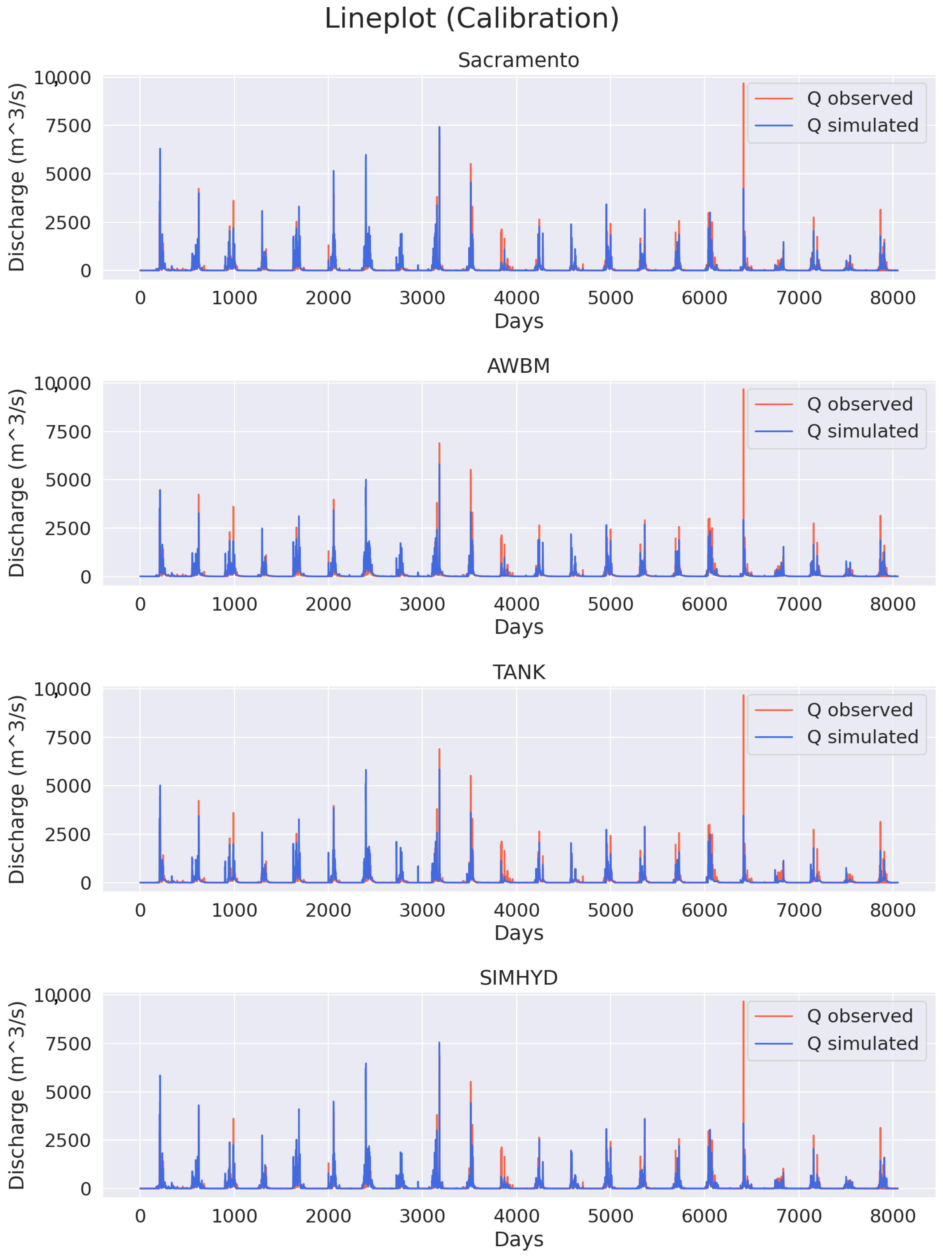
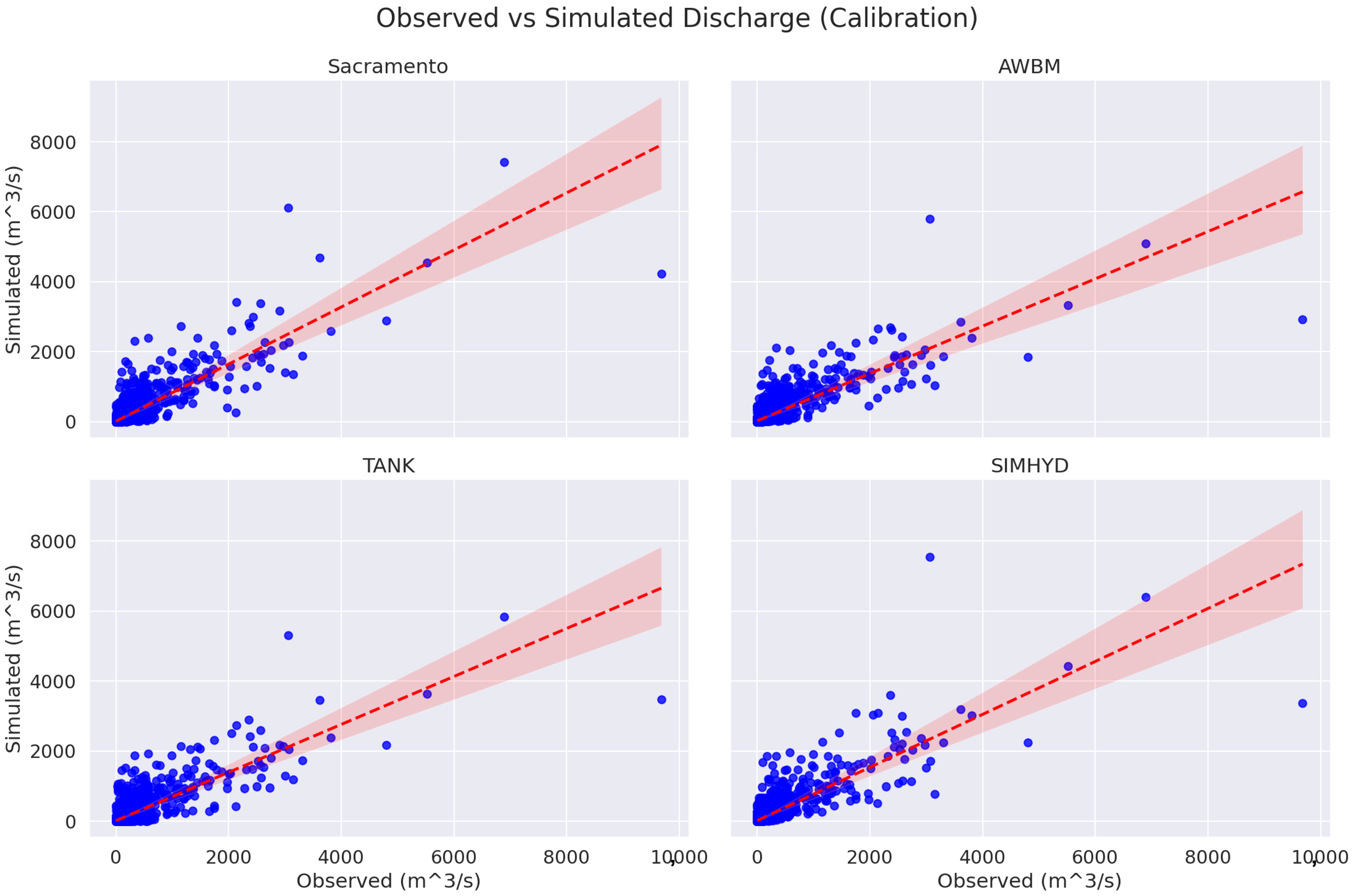
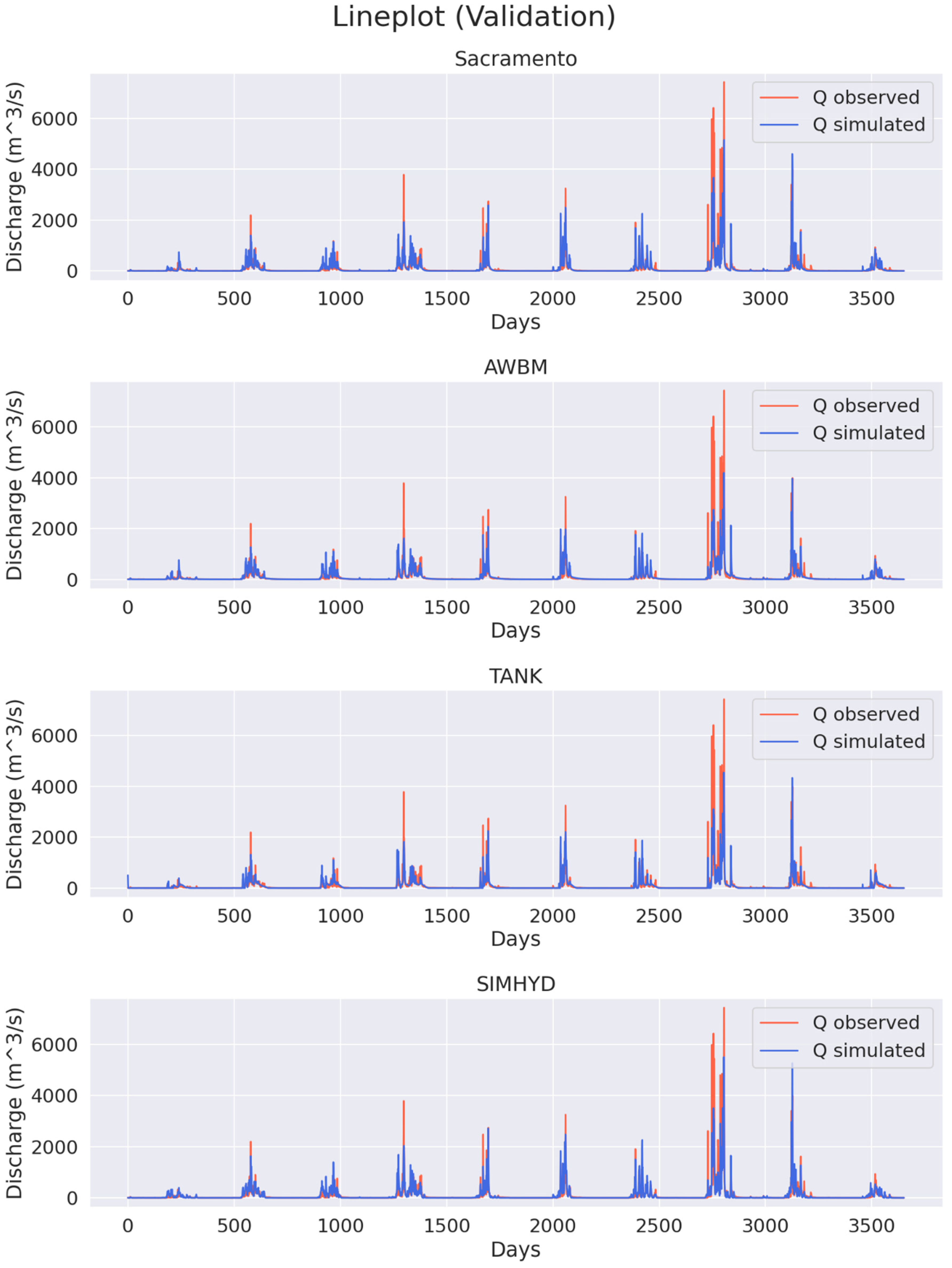
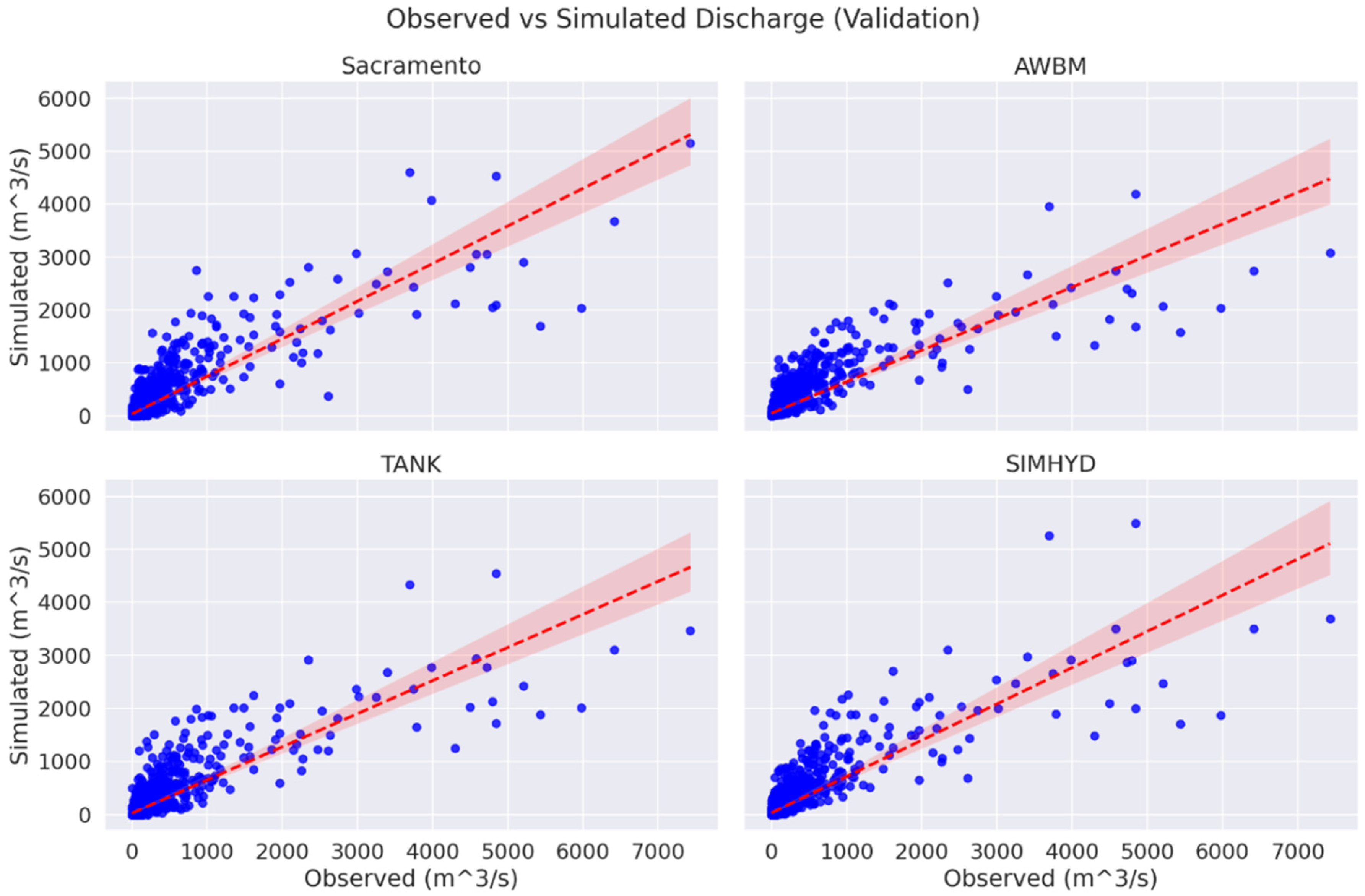
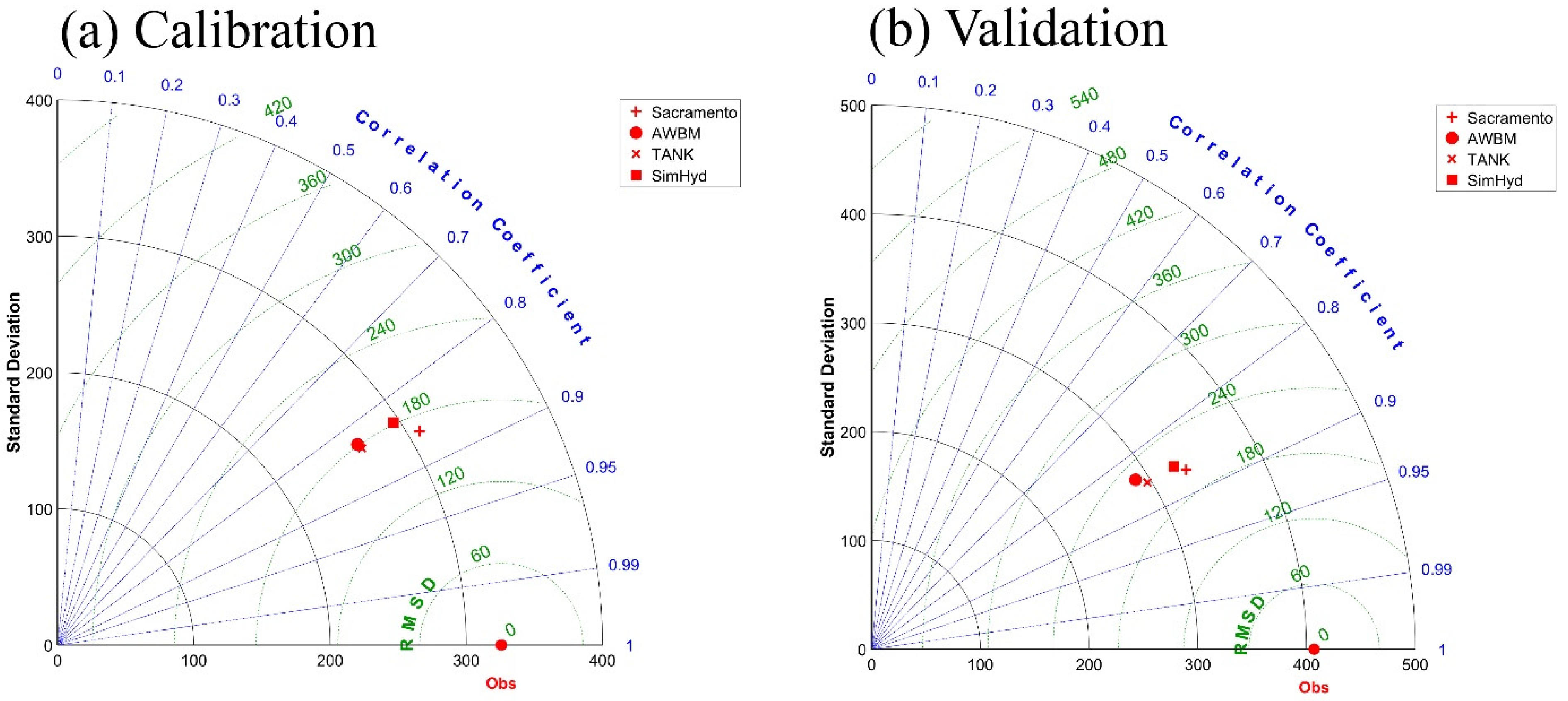
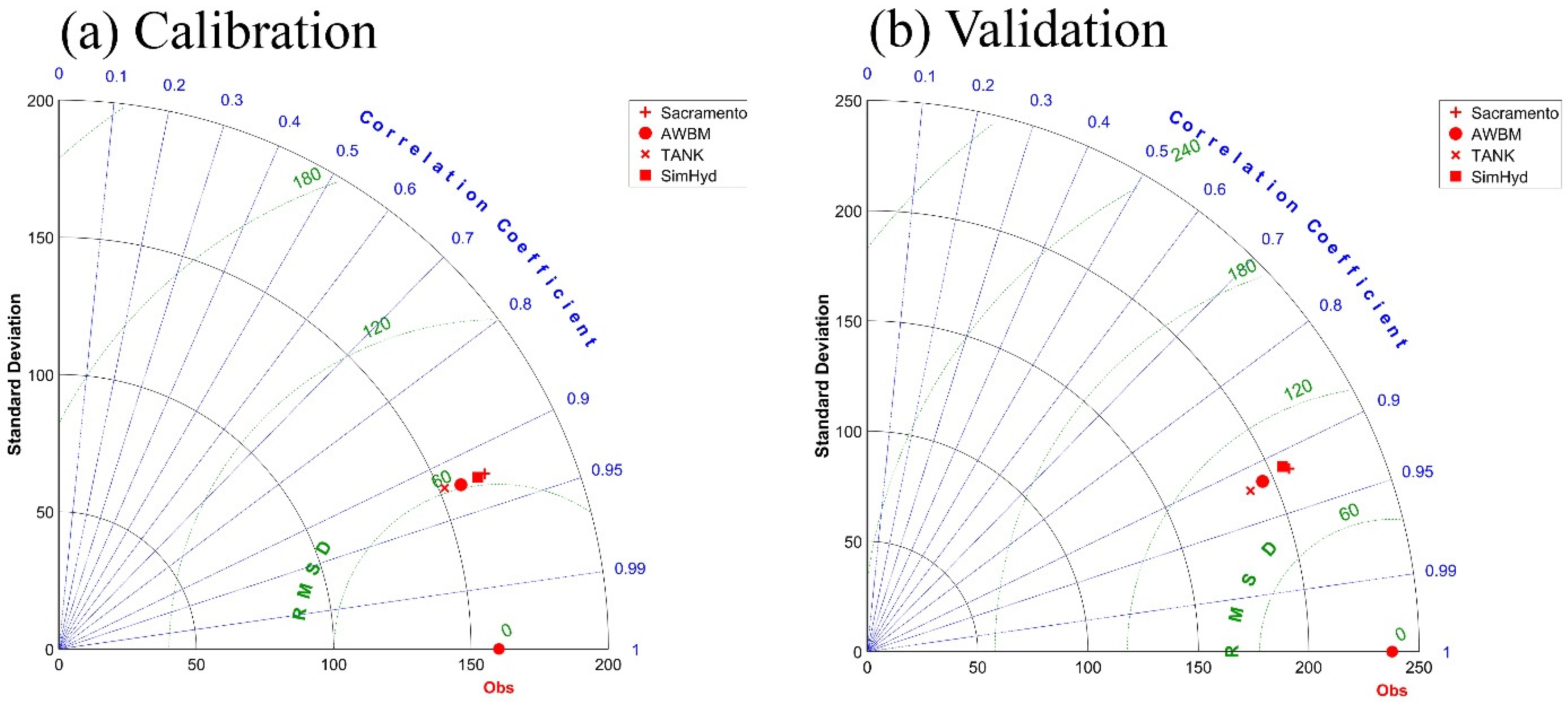
3.1. Evaluation of Conceptual Models

This study evaluated the performance of four different Conceptual streamflow models, namely Sacramento, AWBM, TANK, and SIMHYD, for the Pranhita basin at Rajegaon station. The total period considered is from 1 January 1987 to 19 January 2019. Within this period, a specific time range has been identified as the calibration period, which runs from 1 January 1997 to 19 January 2019. This calibration period has been chosen to cover all types of flows. After the calibration period, the remaining time range, which runs from 1 January 1987 to 31 December 1996, has been designated as the validation period. This validation period is used to test the accuracy and reliability of the model or methodology developed during the calibration period. In this study, the data are split into two parts, in the ratio of 70:30 (Calibration: Validation). This method helps to ensure that the model is not overfitting to the data and that its predictions are robust and accurate. Overall, by specifying the time periods and ratios used in the calibration and validation process, the study ensures its results are reliable and applicable to the entire period under consideration. Descriptive statistics of the data during calibration and validation are mentioned in Table S5 in the Supplementary Material. This study uses GA to find the best values for the parameters [57]. By hard coding the parameter set, the GA queries and operates on a population of observations rather than the parameter values themselves, and Probabilistic rules govern the changes. The settings of the evolutionary algorithm utilized to optimize the research area are as follows: maximum iterations 100, Prob. Mutation 0.01, Nb. Points 40, and Trapezoidal PDF = 2. Table S6 represents the calibrated parameter values for all the conceptual models used in this study.

The performance metrics used for the evaluation were CC, CD, NSE, and RMSE.

Table 2. CC, CD, NSE, and RMSE for Sacramento, AWBM, TANK, and SIMHYD models for daily streamflow.

Model	Calibration				Validation
	CC	CD	NSE	RMSE (m3/s)	CC	CD	NSE	RMSE (m3/s)
Sacramento	0.86	0.74	0.73	168.04	0.87	0.76	0.75	202.61
AWBM	0.83	0.69	0.69	181.16	0.84	0.71	0.69	226.36
TANK	0.84	0.71	0.70	177.28	0.86	0.73	0.72	216.85
SIMHYD	0.83	0.70	0.69	181.44	0.86	0.73	0.73	211.99

represents evaluation metrics for daily streamflow modeling. During the calibration process, the Sacramento model achieved a CC of 0.861, CD of 0.741, NSE of 0.734, and RMSE of 168.03 m³/s. These values indicate that the model fits the observed streamflow data well to the model parameters. During the validation process, the Sacramento model achieved a CC of 0.869, CD of 0.755, NSE of 0.752, and RMSE of 202.614 m³/s. These values show that the Sacramento model also predicted streamflow for an independent dataset well. The other models also performed reasonably well, with some slightly lower and some slightly higher performance metrics than the Sacramento model. The AWBM model achieved a CC of 0.831 and CD of 0.691 during calibration, an NSE of 0.691, and an RMSE of 181.16 m³/s. During validation, it achieved a CC of 0.842, CD of 0.709, NSE of 0.691, and RMSE of 226.355 m³/s. The TANK model achieved a CC of 0.840 and CD of 0.706 during calibration, an NSE of 0.704, and an RMSE of 177.27 m³/s. During validation, it achieved a CC of 0.856, CD of 0.733, NSE of 0.716, and RMSE of 216.847 m³/s. The SIMHYD model achieved a CC of 0.834 and CD of 0.695 during calibration, an NSE of 0.690, and an RMSE of 181.43 m³/s. During validation, it achieved a CC of 0.856, CD of 0.732, NSE of 0.729, and RMSE of 211.994 m³/s.

Table 3. CC, CD, NSE, and RMSE for Sacramento, AWBM, TANK, and SIMHYD models for monthly streamflow.

Model	Calibration				Validation
	CC	CD	NSE	RMSE (m3/s)	CC	CD	NSE	RMSE (m3/s)
Sacramento	0.93	0.86	0.84	64.14	0.92	0.84	0.84	95.27
AWBM	0.93	0.86	0.85	61.41	0.92	0.84	0.83	97.14
TANK	0.92	0.85	0.85	62.85	0.92	0.85	0.83	97.39
SIMHYD	0.93	0.86	0.85	63.06	0.91	0.83	0.83	97.59

shows the monthly streamflow evaluation during calibration and validation. The Sacramento model yielded a CC of 0.925, CD of 0.855, NSE of 0.84, and RMSE of 64.136. Slightly better performance was observed in the AWBM model with a CC of 0.926, CD of 0.857, NSE of 0.853, and RMSE of 61.412. Meanwhile, the TANK model scored a CC of 0.923, CD of 0.852, NSE of 0.846, and RMSE of 62.847, whereas the SIMHYD model achieved a CC of 0.925, CD of 0.856, NSE of 0.845, and RMSE of 63.06. During the validation process, TANK obtained the highest CC value of 0.922, followed by AWBM with 0.918, Sacramento with 0.917, and SIMHYD with 0.913. Additionally, TANK had the highest CD value of 0.85, with AWBM following at 0.843, Sacramento at 0.841, and SIMHYD at 0.834. The NSE values for all models were relatively similar, ranging from 0.832 to 0.839. Finally, Sacramento had the lowest RMSE value of 95.266 m³/s, followed by AWBM at 97.139 m³/s, TANK at 97.391 m³/s, and SIMHYD at 97.593 m³/s.

Figure 3 represents the line plot between observed and simulated streamflow using various conceptual models during calibration. The first range, with streamflow greater than 3000 m³/s, has observed average streamflow of 4339.42 m³/s, and the modeled values by the Conceptual models are Sacramento: 3947.79 m³/s, AWBM: 2952.35 m³/s, TANK: 3254.00 m³/s, and SIMHYD: 3655.14 m³/s. The second range, with streamflow between 2000 m³/s and 3000 m³/s, has observed average streamflow of 2521.54 m³/s, and the modeled values by the hydrological models are Sacramento: 2315.21 m³/s, AWBM: 1935.45 m³/s, TANK: 2025.39 m³/s, and SIMHYD: 2325.28 m³/s. The third range, with streamflow between 1000 m³/s and 2000 m³/s, has observed average streamflow of 1419.94 m³/s, and the modeled values by the hydrological models are Sacramento: 1612.97 m³/s, AWBM: 1392.39 m³/s, TANK: 1399.47 m³/s, and SIMHYD: 1496.91 m³/s. In the first range of streamflow with values greater than 3000 m³/s, the hydrological models’ performance shows that Sacramento is the most accurate model with a modeled value of 3947.79 m³/s, which is closest to the observed value of 4339.426471 m³/s. The other models, AWBM, TANK, and SIMHYD, have modeled values of 2952.35 m³/s, 3254.00 m³/s, and 3655.14 m³/s, respectively.

To further study the forecasting accuracy during calibration, scatterplots for daily streamflow have been drawn for all the models shown in Figure 4, in which the Sacramento simulation is very close to observed streamflow values. The various conceptual models with correlation coefficients are relatively high (above 0.83), suggesting a strong positive linear relationship between the compared models. This means that the data points on the scatter plot will be tightly clustered around the 45° line, indicating that the models are highly correlated with observed streamflow.

Figure S5 explains FDC (Flow Duration Curve) during calibration, which is a graphical representation of the probability distribution of streamflow. It is constructed by plotting the discharge values against their corresponding exceedance probabilities. Essentially, the FDC provides information about the percentage of time that a particular flow rate is equaled or exceeded, offering a probabilistic description of stream flow at a Rajegaon station. The Sacramento model is generally consistent with the observed streamflow, except for underestimated values that can reach up to 2000 m³/s and overestimates in the range of 400–1000 m³/s of streamflow values. Similar patterns are also seen in the results of the AWBM model. On the other hand, the TANK and SIMHYD models exhibit a similar trend, showing better prediction for medium flows but poor performance for peak flow simulation compared to the Sacramento and AWBM models.

Similarly, Figure 5 denotes the line plot between observed and modeled flows during validation, indicating that all four models performed well in capturing the flow patterns, especially during peak events. However, the Sacramento model performs best among the four models, producing the closest match to the observed flows for peak events. The other models (AWBM, TANK, and SIMHYD) also performed well but with slightly higher deviations from the observed flows. For predicting streamflow during high flows (>2000 m³/s), the results suggest that all four models performed reasonably well, with average streamflow predictions ranging from 2171.57 m³/s to 2426.21 m³/s. The Sacramento model has the best overall performance for predicting high flows, with the lowest deviation from the observed streamflow.

CC ranges from 0.8418 to 0.8688 during validation, indicating a moderate to strong positive correlation between the observed streamflow and the modeled streamflow for each of the four models. This result suggests that the modeled streamflow generally agrees with the observed streamflow, with the scatter of data points relatively close to a straight line observed in Figure 6.

The FDC plot during validation, depicted in Figure S6, illustrates that the Sacramento model performs fairly well in reproducing observed streamflow. However, it tends to underestimate streamflow values in the peak time and overestimate those above 500–1500 m³/s. Similar patterns are observed in the results of the AWBM model. Conversely, the TANK and SIMHYD models display better accuracy in predicting medium flows but exhibit poorer performance in simulating peak flows than the Sacramento and AWBM models.

Figure 7 compares different hydrological models (Sacramento, AWBM, TANK, and SIMHYD) against observed data using Taylor’s diagram during both calibration and validation for daily streamflow modeling. Taylor’s diagram is a graphical tool that compares multiple models with respect to their CC, standard deviation (SD), and RMSE to the observed data. It provides a quick visual assessment of how well a model captures the variation and pattern in the observed data. In the case of Figure 7a, during calibration, clearly observed that all models have a CC ranging from 0.83 to 0.86, indicating a good level of agreement between the model outputs and the observed data. However, when comparing the SD values, we can observe that the AWBM and TANK models have lower values than the other models, indicating that they tend to underestimate the variability of the observed data. In comparison, the Sacramento model showed a very close SD of 308.59. The RMSE values for all models range between 168.04 and 181.44 m³/s, with the Sacramento model having the lowest RMSE value, indicating that it has the best agreement with the observed data in terms of absolute errors.

Referring to Figure 7b, it can be observed that the SDs of the predicted values for the Sacramento, AWBM, TANK, and SIMHYD hydrological models are 332.98, 288.44, 296.36, and 324.74, respectively. The CC between the observed and predicted values are 0.87, 0.84, 0.86, and 0.86, respectively. Additionally, RMSE values, which are 202.61, 226.35, 216.85, and 211.99 m³/s, are included in the Taylor diagram. Based on the SD, the Sacramento model appears to perform the best, as it is the closest to the observed value. Furthermore, based on the RMSE and CC values, the Sacramento model is found to be the best for the daily streamflow simulating models during the validation period.

Figure 8a represents the Taylors’ diagram during calibration for monthly streamflow simulation. All four models have similar CC values of around 0.925, indicating a strong linear relationship with the observed data. The RMSE values are also relatively close, ranging from 61.412 to 64.136. However, the observed SD is 160.61, which is significantly lower than the SDs of the models (ranging from 152.60 to 168.02). This indicates that the models may not accurately capture the variability of the observed data, even though they have a strong linear relationship and low RMSE.

Figure 8b shows Taylor’s diagram for monthly streamflow simulation validation. The values indicate that the Sacramento model has the highest CC (0.917), indicating a good correlation between the model and the observed data. However, the RMSE of 95.27 m³/s and SD of 209.171 is much closer to the observed streamflow values, indicating some error in the model’s predictions. The other models, namely AWBM, TANK, and SIMHYD, have similar CC values, but their RMSE and SD values differ slightly. The AWBM model has a slightly higher RMSE of 97.14 m³/s and a lower SD of 195.81 compared to the TANK and SIMHYD models, which are far lower than the observed streamflow data. The TANK model has a slightly lower RMSE of 97.39 and an SD of 189.09. The SIMHYD model has the lowest RMSE of 97.59 m³/s but the highest SD of 206.87. Overall, the information provided in Table 2 and Table 3 suggests that the Sacramento model performs the best in terms of RMSE, CC, and SD, while all models show a relatively good correlation with the observed data for daily and monthly streamflow simulation.

3.2. Future Rainfall and Temperature Projections

3.2.1. Monthly Rainfall Projections

The monthly rainfall amounts for the four different scenarios are depicted in Figure S7: (a) SSP126, (b) SSP245, (c) SSP370, and (d) SSP585. This figure implies that there will be a rise in rainfall across all possible forthcoming time frames during July, August, September, and October. The Supplementary Material comprises a comprehensive analysis of the increase in rainfall.

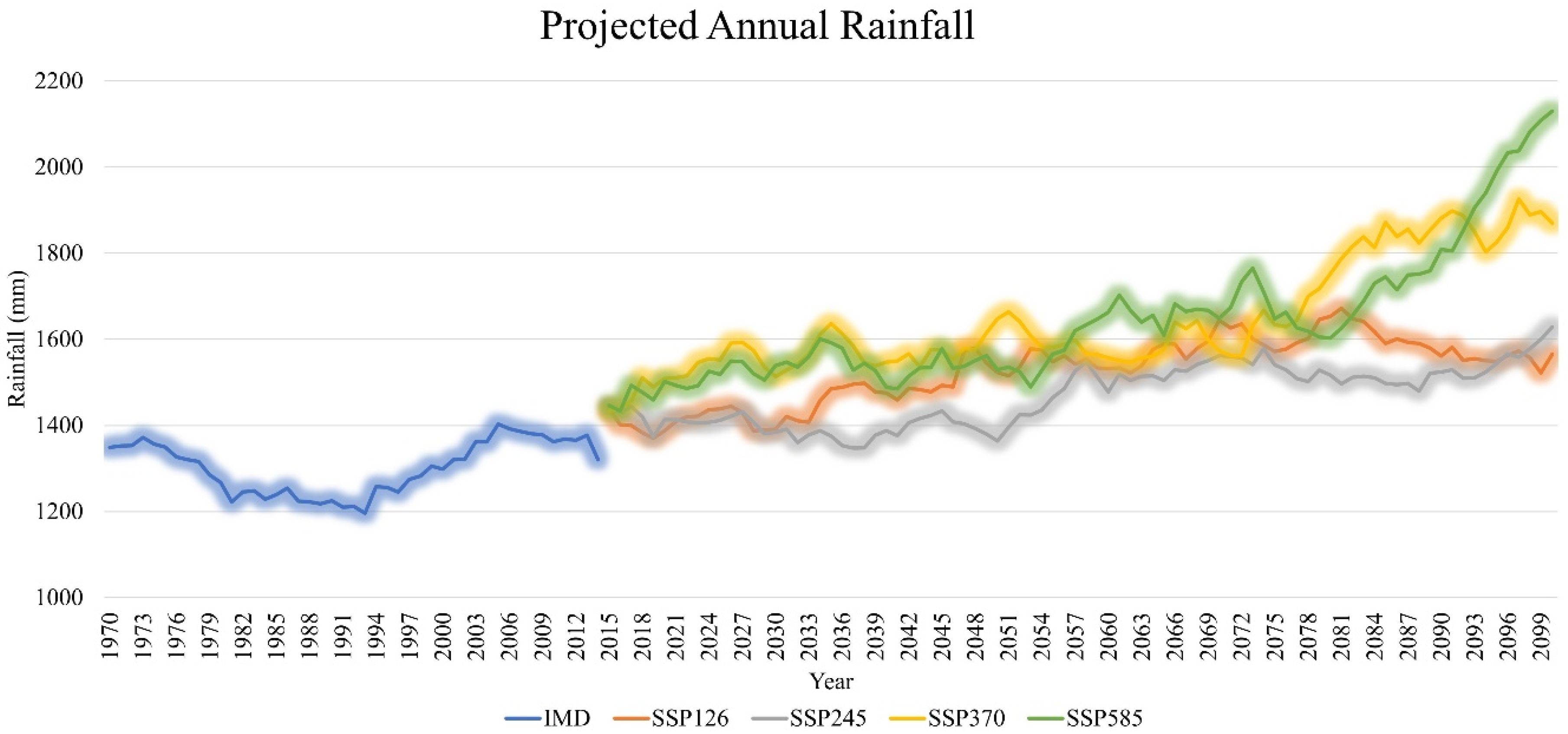
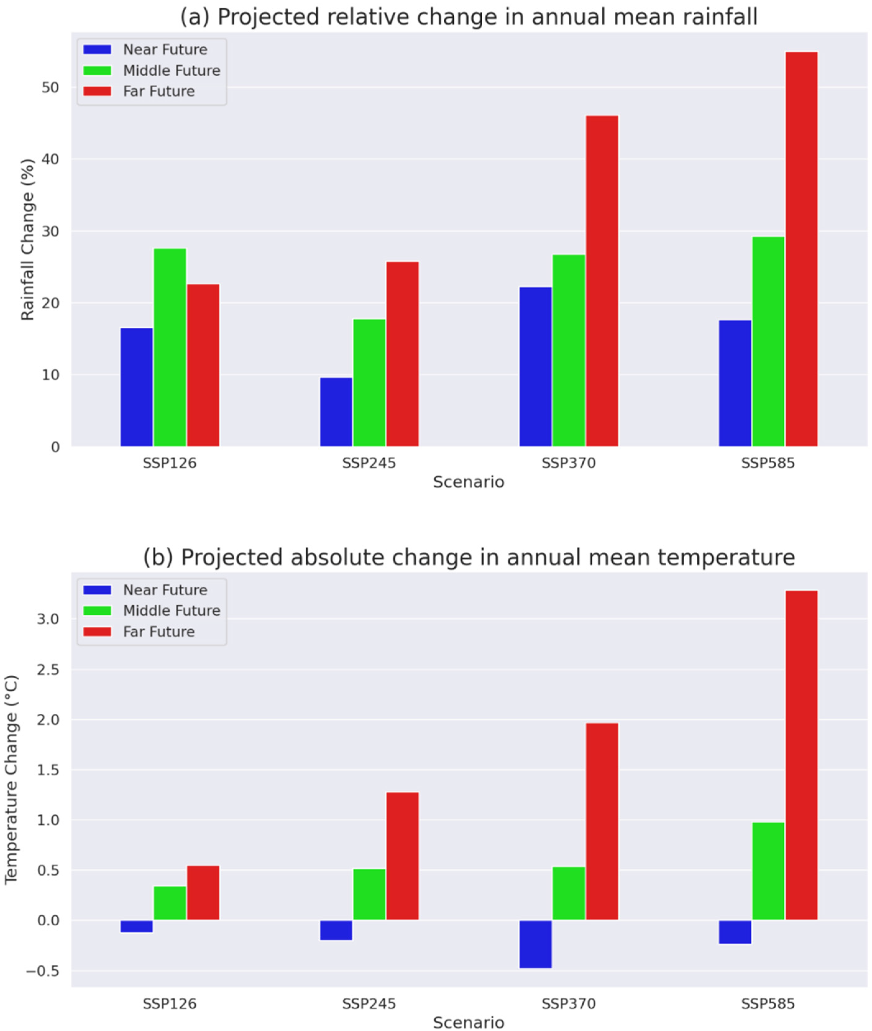
3.2.2. Annual Rainfall and Temperature Projections

Figure 9 depicts a line plot illustrating the 20 year annual rolling mean of rainfall data obtained from IMD and EC-Earth3 sources. The data collected from IMD cover the period from 1970 to 2015, which serves as the base period for the analysis. The future projections from 2015 to 2100 were obtained from EC-Earth3 for the SSP126, SSP245, SSP370, and SSP585 scenarios. The observed data demonstrate fluctuations between 1200 mm to 1400 mm during the 1970 to 2015 timeframe, whereas the future projections indicate an increasing trend across all the scenarios. Notably, the SSP370 and SSP585 scenarios depict an exponential increase in rainfall in the far future, ranging from 1600 mm to 2200 mm.

Figure 10a represents the relative change in the annual mean rainfall, In the near future, SSP370 has the highest relative change in rainfall (22.25%), followed by SSP585 (17.64%), SSP126 (16.57%), and SSP245 (9.67%). This suggests that the SSP370 scenario is likely to experience the most significant increase in rainfall in the near future. In the middle future, SSP585 has the highest relative change in rainfall (29.24%), followed by SSP370 (26.74%), SSP245 (17.78%), and SSP126 (27.64%). This indicates that the SSP585 scenario is likely to experience the most significant increase in rainfall in the middle future. In the far future, SSP585 has the highest relative change in rainfall (55.02%), followed by SSP370 (46.09%), SSP245 (25.78%), and SSP126 (22.64%). This suggests that the SSP585 scenario will likely experience the most significant increase in rainfall in the future. Overall, the data suggest that the SSP585 scenario is likely to experience the most significant increase in rainfall across all three time periods, while SSP370 is also projected to have a relatively high increase in rainfall, especially in the far future.

Figure 10b represents the absolute change in the annual mean temperature. Looking at the plot, the trend in the absolute change in annual mean temperature is generally upward, with increasing values over time and across scenarios. In the near future, the values range from a decrease of −0.12 °C (under SSP126) to a decrease of −0.48 °C (under SSP370). However, in the middle future and far future, the values are all positive, indicating an overall increase in temperature compared to a baseline. In the middle future, the values range from 0.34 °C (under SSP126) to 0.98 °C (under SSP585). In the far future, the values range from 0.54 °C (under SSP126) to 3.29 °C (under SSP585), with larger absolute changes compared to the middle future. The largest absolute change is seen under the SSP585 scenario, which assumes a high level of greenhouse gas emissions and rapid technological growth. Overall, these data highlight the potential impacts of different SSPs on future temperature trends, with more aggressive emissions scenarios leading to larger temperature increases. They also suggest that the effects of these pathways may not be immediate, with larger changes seen in the middle future and far future.

3.3. Projected Changes in Streamflow

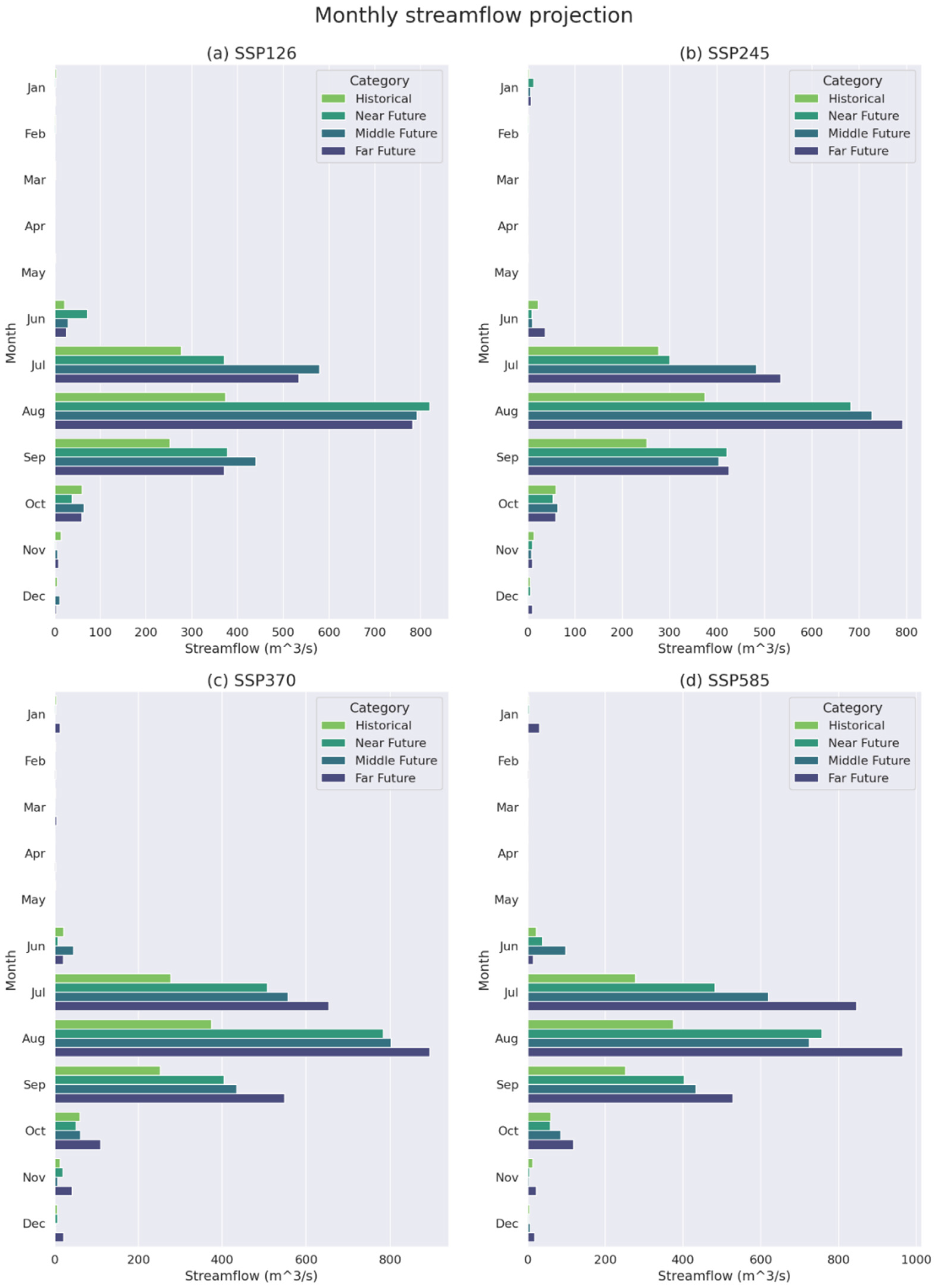
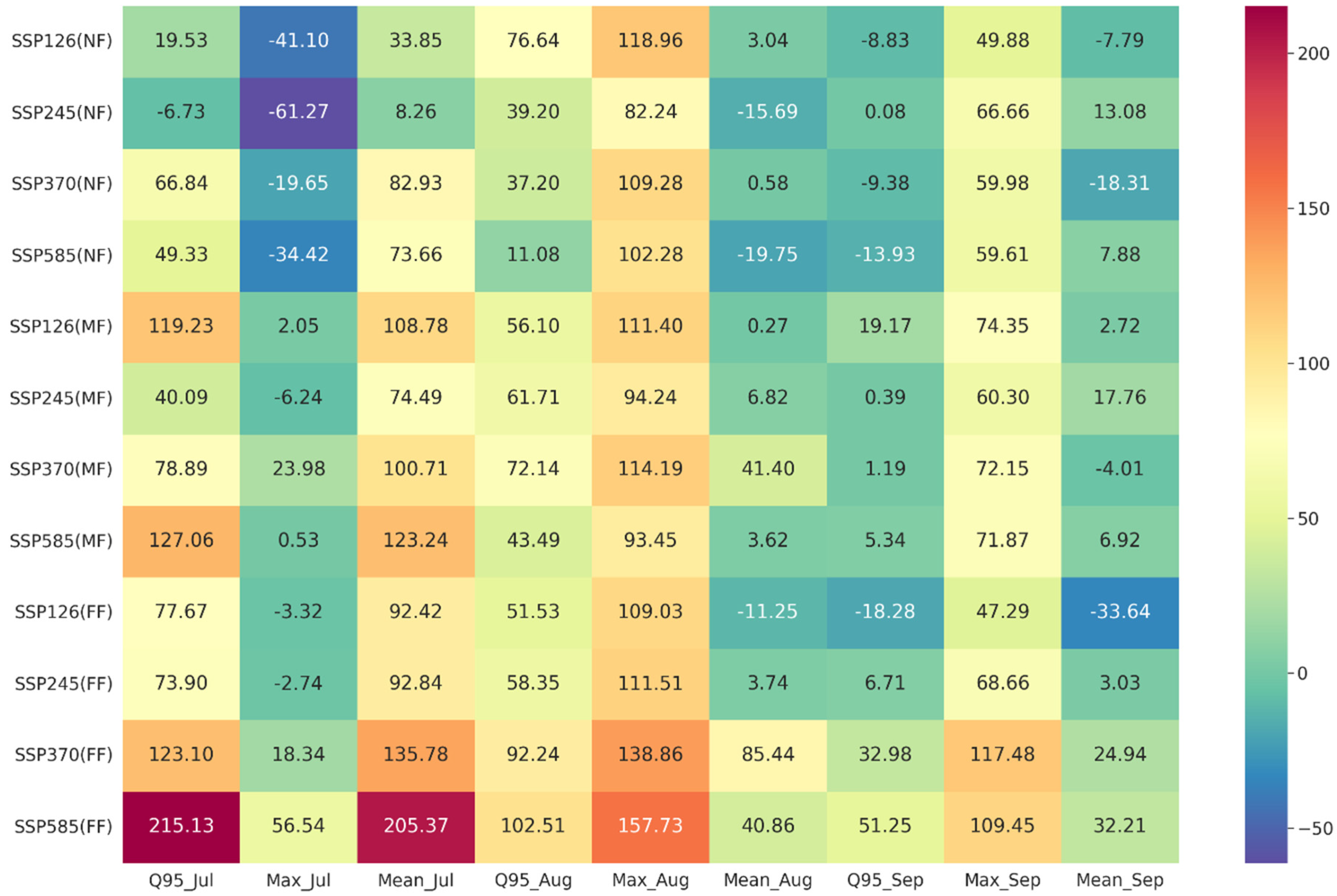
3.3.1. Monthly Streamflow Projections

Figure 11 depicts the monthly average streamflow for the four distinct scenarios: (a) SSP126, (b) SSP245, (c) SSP370, and (d) SSP585.

Figure 11a represents the monthly average streamflow projection for the SSP126 scenario. In June, the historical average streamflow was 22.67 m³/s, which is significantly lower than the near- and middle-future averages of 71.77 and 30.34 m³/s, respectively. The far future average for June is slightly lower at 26.40 m³/s. For July, the historical average streamflow is 277.41 m³/s, which increases to 371.31 and 579.17 m³/s in the near and middle future, respectively. The far future average for July is slightly lower at 533.79 m³/s. In August, the historical average streamflow was 374.57 m³/s, which will significantly increase to 820.14 m³/s in the near future. August’s middle and far future averages are slightly lower at 791.85 and 782.95 m³/s, respectively. The historical average streamflow for September is 252.30 m³/s, which will increase to 378.15 m³/s in the near future. The September middle and far future averages are 439.88 and 371.60 m³/s, respectively. In October, the historical average streamflow was 60.68 m³/s, which is lower than the near-future average of 38.26 m³/s. The middle- and far-future averages for October are higher at 64.28 and 59.30 m³/s, respectively.

Figure 11b displays the monthly average streamflow projection for the SSP245 scenario. For June, the historical average of 22.67 m³/s decreases to 9.28 m³/s in the near future but shows an increase to 10.90 and 36.97 m³/s in the middle and far future, respectively. In July, the historical average of 277.41 m³/s increases to 300.33 m³/s in the near future and further increases to 484.07 and 534.96 m³/s in the middle and far future, respectively. For August, the historical average of 374.57 m³/s shows a significant increase to 682.63 m³/s in the near future, and the middle and far future averages for August are 727.57 m³/s and 792.24 m³/s, respectively. In September, the historical average of 252.30 m³/s increases to 420.47 m³/s in the near future, and the middle and far future averages are 404.44 m³/s and 425.54 m³/s, respectively. For October, the historical average of 60.68 m³/s shows a slight decrease to 53.84 m³/s in the near future but increases to 64.16 m³/s and 59.80 m³/s in the middle and far future, respectively.

Figure 11c displays the monthly average streamflow projections for the SSP370 scenario. For June, the historical average of 22.67 m³/s decreases to 9.11 m³/s in the near future but increases significantly to 45.22 m³/s and 20.87 m³/s in the middle and far future, respectively. In July, the historical average of 277.41 m³/s increases significantly to 507.46 m³/s in the near future and further increases to 556.79 m³/s and 654.07 m³/s in the middle and far future, respectively. For August, the historical average of 374.57 m³/s will increase significantly to 783.88 m³/s in the near future. August’s middle and far future averages are 802.27 m³/s and 894.68 m³/s, respectively. In September, the historical average of 252.30 m³/s increases to 403.62 m³/s in the near future. The September middle and far future averages are 434.34 m³/s and 548.71 m³/s, respectively. For October, the historical average of 60.68 m³/s decreases slightly to 51.64 m³/s in the near future but increases to 62.29 m³/s and 110.55 m³/s in the middle and far future, respectively.

Figure 11d displays the monthly average streamflow projections for the SSP585 scenario. In January, the historical average of 3.94 m³/s increases to 5.23 m³/s in the near future and further increases to 1.32 m³/s and 30.34 m³/s in the middle and far future, respectively. For June, the historical average of 22.67 m³/s increases to 39.00 m³/s in the near future and further increases significantly to 98.20 m³/s and 15.08 m³/s in the middle and far future, respectively. In July, the historical average of 277.41 m³/s increases significantly to 481.75 m³/s in the near future and further increases to 619.29 m³/s and 847.14 m³/s in the middle and far future, respectively. For August, the historical average of 374.57 m³/s increases significantly to 757.67 m³/s in the near future, with the middle and far future averages being 724.62 m³/s and 965.38 m³/s, respectively. In September, the historical average of 252.30 m³/s increases to 402.71 m³/s in the near future, with the middle and far future averages being 433.63 m³/s and 528.45 m³/s, respectively. Lastly, for October, the historical average of 60.68 m³/s slightly decreases to 58.89 m³/s in the near future but increases to 85.57 m³/s and 118.46 m³/s in the middle and far future, respectively.

Figure 12a–c show whisker plots for July, August, and September for each of the baseline and SSP scenarios (SSP126, SSP245, SSP370, and SSP585), across all near future (NF), middle future (MF), and far future (FF) timeframes. The box in the plot represents the middle 50% of the data, with the median value shown as a line inside the box. The interquartile range (IQR), which is the distance between the first quartile (Q1) and the third quartile (Q3), is represented by the length of the box. The whiskers extend from the box and show the range of the data, usually from the minimum to the maximum values that are not considered outliers. Outliers, data points outside the whiskers, are shown as individual points on the plot. The whiskers’ exact range depends on the box plot’s specific implementation, with some implementations extending them to other values, such as the 5th and 95th percentiles.

Figure 13 shows the heatmap of the relative change (%) in comparison to the baseline for the 95th percentile, maximum, and mean values of monthly streamflow. The comparison is made for the four SSPs (SSP126, SSP245, SSP370, and SSP585) and for three different time periods: near future (NF), middle future (MF), and far future (FF).

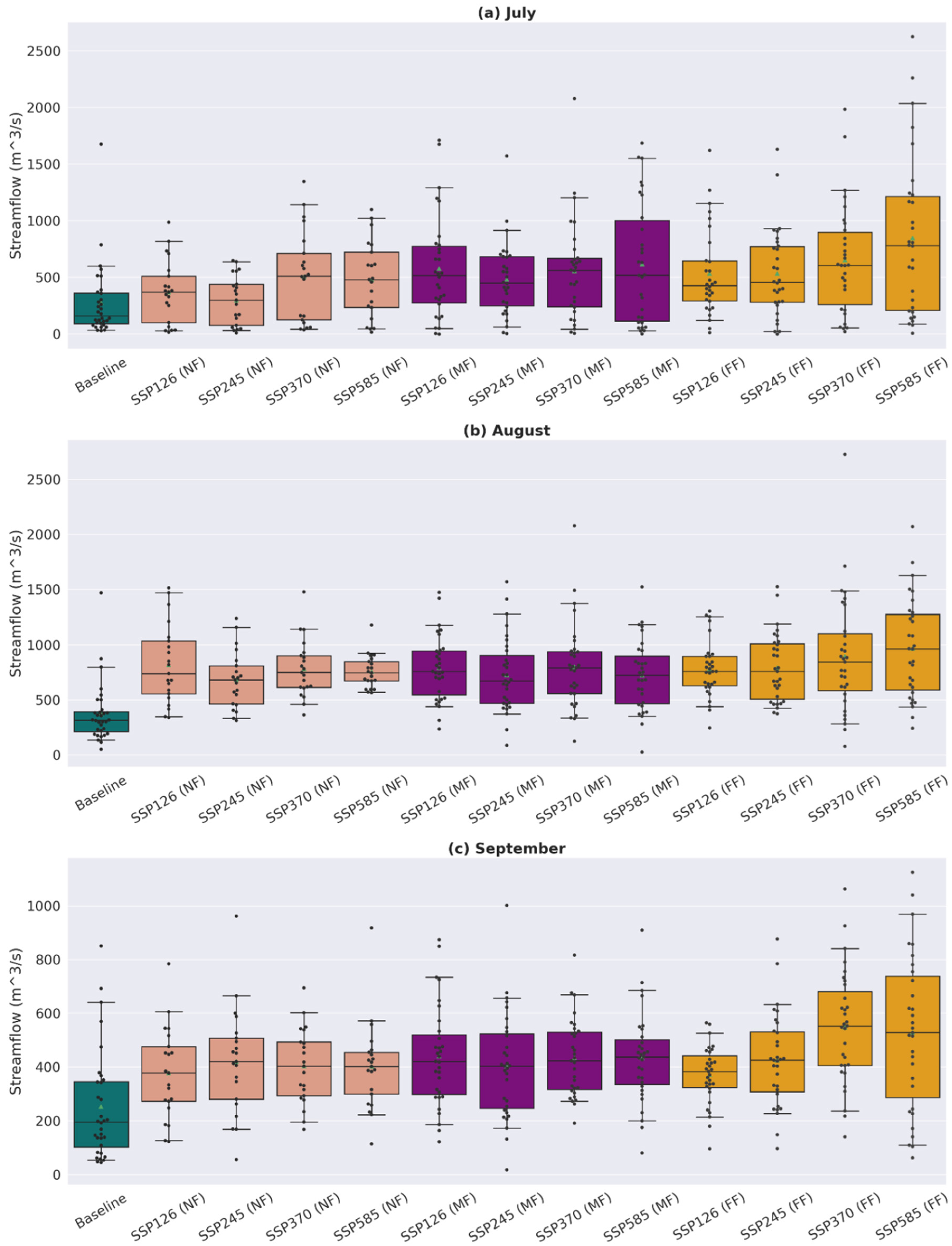
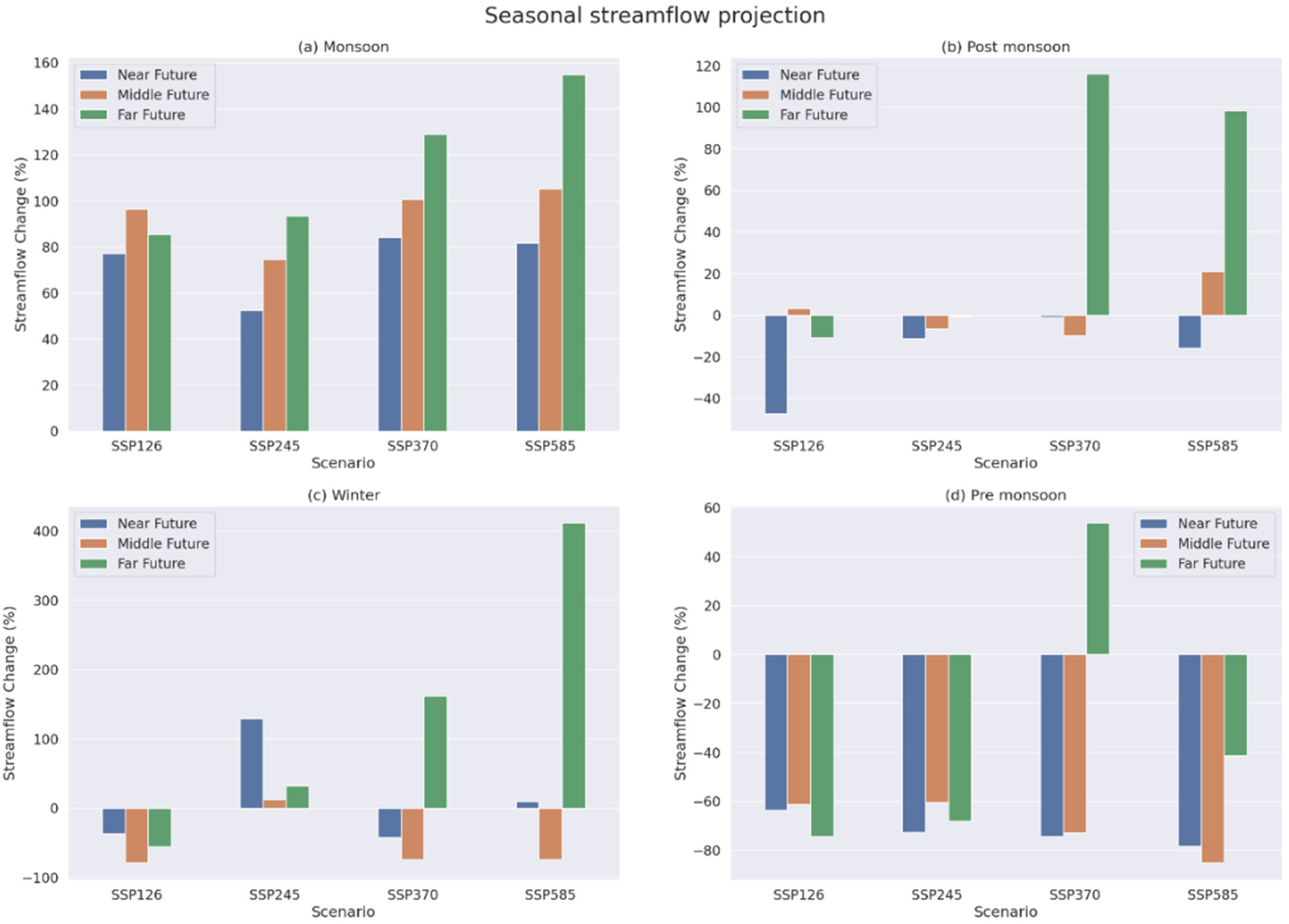
3.3.2. Seasonal streamflow projections

Figure 14 depicts the seasonal streamflow projections for the four distinct scenarios: (a) Monsoon, (b) Post-monsoon, (c) Winter, and (d) Pre-monsoon.

Monsoon

For the near future, SSP370 and SSP585 scenarios show an increase in monsoon streamflow relative to the baseline, with SSP370 showing the highest increase at 84.16%, while SSP126 and SSP245 scenarios show a decrease in streamflow compared to other scenarios. For the middle future, all scenarios show an increase in monsoon streamflow relative to the baseline, with SSP585 showing the highest increase at 105.10% and SSP126 showing the lowest increase at 96.19%. For the far future, SSP370 and SSP585 scenarios show a significant increase in monsoon streamflow relative to the baseline, with SSP585 showing the highest increase at 154.72%, while SSP126 and SSP245 scenarios show a decrease in streamflow. Overall, the SSP585 scenario shows the highest increase in monsoon streamflow in all three future timeframes, while the SSP126 scenario shows a decrease in streamflow in all three future timeframes.

Post-Monsoon

In the near future, all four scenarios are projected to result in a decrease in monsoon streamflow. The SSP370 scenario shows the smallest decrease of only 1.13%, while the SSP126 scenario shows the largest decrease of 47.62%. In the middle future, the SSP585 scenario shows a significant increase in monsoon streamflow of 20.92%, while the other three scenarios continue to show a decrease, with SSP370 showing the smallest decrease of 9.99%. In the far future, the SSP370 and SSP585 scenarios show a significant increase in monsoon streamflow of 115.97% and 98.16%, respectively, while the other two scenarios show a decrease. The SSP126 scenario shows the largest decrease of 11.01%. Overall, the data suggest that post-monsoon streamflow is likely to decrease in the near future, but the trend may reverse in the middle and far future for some scenarios.

Winter

In the near future, SSP126 will show a decrease in streamflow of 36.87%, while SSP245 will show a significant increase in streamflow of 128.85%. SSP370 shows a decrease in streamflow of 42.16%, while SSP585 shows a small increase in streamflow of 8.73%. In the middle future, all scenarios show an increase in monsoon streamflow relative to the baseline. However, the magnitude of change varies significantly between the scenarios. SSP126 shows a larger decrease of 79.10%, while SSP245 shows a slight increase of 12.57%. SSP370 shows a larger decrease of 74.35%, and SSP585 shows a larger decrease of 74.61%. In the far future, the changes in streamflow will become more extreme. SSP126 shows a smaller decrease of 55.69%, while SSP245 shows a significant increase of 31.80%. SSP370 shows a significant increase of 161.57%, and SSP585 shows a significant increase of 411.64%. Notably, the percentage changes in streamflow can be quite significant, ranging from a decrease of 79.10% to an increase of 411.64%, depending on the chosen scenario and time period.

Pre-Monsoon

In the near future, all scenarios show a decrease in streamflow compared to the baseline scenario. SSP126 shows the highest decrease at 63.55%, followed by SSP245 with a decrease of 72.64%. SSP370 and SSP585 show similar decreases of 74.52% and 78.49%, respectively. In the middle future, SSP126 and SSP245 scenarios show a smaller decrease in streamflow compared to the baseline scenario, with a change of 61.44% and 60.58%, respectively. SSP370 shows a larger decrease of 72.83%, while SSP585 shows the largest decrease of 85.19%. In the far future, SSP126 and SSP245 scenarios show an increase in streamflow relative to the baseline scenario, with changes of 74.63% and 68.14%, respectively. SSP370 shows a significant increase of 53.80%, while SSP585 shows a decrease of 41.47%. The SSP370 and SSP585 scenarios show the most decrease in streamflow.

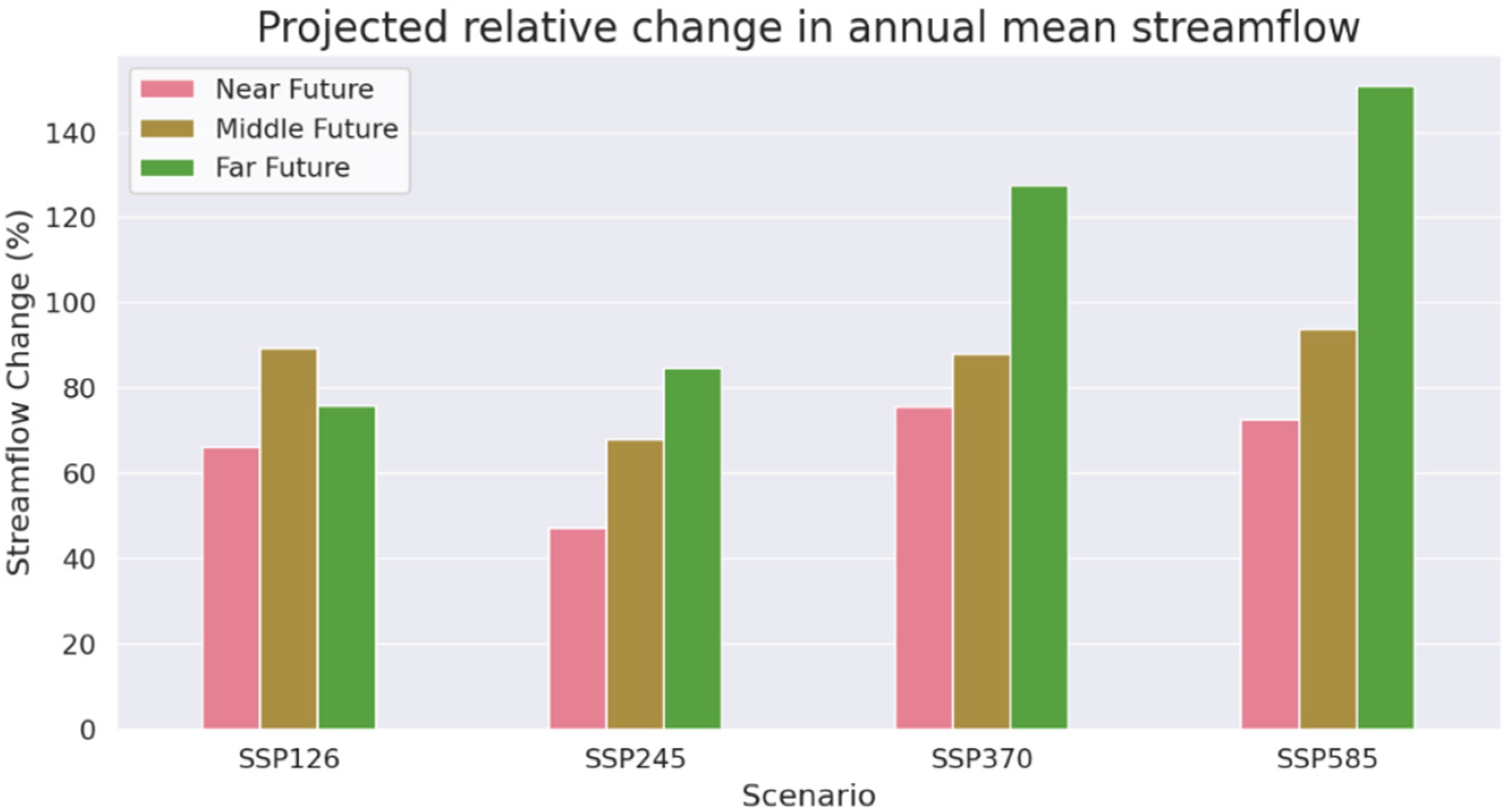
3.3.3. Annual Streamflow Projection

Figure 15 portrays the projected relative change in annual mean streamflow for the four distinct scenarios: SSP126, SSP245, SSP370, and SSP585. According to the SSP126 scenario, the annual relative change in streamflow is expected to increase by 66.03% in the near future, 89.28% in the middle future, and 75.91% in the far future. Under the SSP245 scenario, it is projected that the annual relative change in streamflow will increase by 47.12% in the near future, 67.92% in the middle future, and 84.73% in the far future. For the SSP370 scenario, it is anticipated that the annual relative change in streamflow will increase by 75.70% in the near future, 87.89% in the middle future, and 127.48% in the far future. Finally, the SSP585 scenario suggests that the annual relative change in streamflow will increase by 72.49% in the near future, 93.80% in the middle future, and 150.76% in the far future. Overall, all scenarios indicate an increase in streamflow in all three time periods, but the magnitude and rate of increase vary between scenarios. Of all the scenarios, SSP370 and SSP585 suggest the highest streamflow increase rates in all three time periods.

4. Discussion

In recent years, the Pranhita sub-basin has faced several challenges due to increasing human activities such as deforestation, mining, and water extraction for agriculture and industrial purposes. These activities have led to soil erosion, forest cover loss, and water quality degradation. Additionally, climate change is expected to further impact the sub-basin by altering rainfall patterns and increasing the frequency and intensity of extreme weather events.

The present investigation employs four lumped conceptual models, namely Sacramento, AWBM, TANK, and SIMHYD, to simulate streamflow for the Pranhita basin at Rajegaon station during the period spanning 1987 to 2019. The accuracy of these models is evaluated using performance metrics such as CC, CD, NSE, and RMSE. The conceptual model utilizes rainfall and PET as inputs to simulate streamflow, with PET being derived from maximum and minimum temperatures. To summarize, conceptual models illustrate the nonlinear correlation between effective rainfall and streamflow. The optimization of the parameters of the conceptual model was carried out through the utilization of GA. The objective function employed in this investigation was NSE. The results indicate that the Sacramento model exhibited superior performance in daily streamflow modeling, as evidenced by its highest accuracy scores in both calibration and validation. Specifically, the model demonstrated the lowest RMSE and the highest CC, CD, and NSE values. During the calibration process, the Sacramento model achieved a CC of 0.861, CD of 0.741, NSE of 0.734, and RMSE of 168.03 m3/s. During validation, it achieved a CC of 0.869, CD of 0.755, NSE of 0.752, and RMSE of 202.614 m³/s. The other models also performed reasonably well, with some slightly lower and some slightly higher performance metrics than the Sacramento model. Overall, the Sacramento model demonstrated superior performance in fitting the observed streamflow data to the model parameters and in predicting streamflow for an independent dataset [58].

The monthly rainfall predictions for four scenarios, historical and SSP126, SSP245, SSP370, and SSP585, were analyzed. The SSP585 scenario shows the most significant changes in rainfall patterns across different time periods. In January, the historical average rainfall was 13.17 mm, which increased to 31.38 mm in the far future under the SSP585 scenario. February’s historical average was 10.26 mm, which could decrease to 5.15 mm in the near future before increasing to 14.93 mm in the far future. In June, the historical average rainfall was 177.85 mm, which decreased significantly to 70.62 mm in the near future under the SSP585 scenario before increasing significantly to 140.52 mm in the middle future and slightly decreasing to 58.72 mm in the far future. In July, the historical average rainfall was 418.90 mm, which slightly decreased in the near future to 491.75 mm under the SSP585 scenario before increasing further to 679.12 mm in the far future. September’s historical average was 195.66 mm, which significantly increased to 349.69 mm in the far future under the SSP585 scenario. Finally, in December, the historical average was 7.67 mm of rainfall, which significantly increased to 41.41 mm in the far future under the SSP585 scenario. In the near future, SSP370 has the highest relative change in rainfall (22.25%), followed by SSP585 (17.64%), SSP126 (16.57%), and SSP245 (9.67%). In the middle future, SSP585 has the highest relative change in rainfall (29.24%), followed by SSP370 (26.74%), SSP245 (17.78%), and SSP126 (27.64%). In the far future, SSP585 has the highest relative change in rainfall (55.02%), followed by SSP370 (46.09%), SSP245 (25.78%), and SSP126 (22.64%). The largest absolute change in annual mean temperature is seen under the SSP585 scenario in the Far Future, with a value of 3.29 °C. According to O’Neill et al. [9] and Masson-Delmotte et al. [59], the SSP585 scenario represents the most extreme pathway of the SSPs, characterized by high greenhouse gas emissions, rapid population growth, and high economic development. This scenario is expected to lead to a global temperature rise of over 4 °C by the end of the century [60]. Climate models predict that this scenario could result in changes in rainfall patterns, with an increase in rainfall in some months and a decrease in others. Several factors could contribute to these changes, including higher global temperatures, changes in atmospheric circulation patterns, more frequent and intense El Niño events, and continued land use changes, such as deforestation and urbanization [61].

The average monthly streamflow for four different SSPs in five months (June to October) was analyzed. SSP126 showed a decrease in historical average streamflow in June but increased in July, August, September, and October. SSP245 decreased in June but increased in the middle and far future. SSP370 decreased in the near future but increased significantly in the middle future and slightly decreased in the far future. SSP585 increased in the near and middle future but decreased significantly in the far future in January and June and increased in the remaining months. The distribution of their monthly streamflow across the simulation period is further analyzed, with a focus on the extremely high streamflow, because the average monthly streamflow is constantly anticipated to grow during the four wet months from July to October (Figure 11). Whisker plots for the three months of streamflow under different climate change scenarios are shown in Figure 12. Whisker plots showing monthly streamflow during the baseline era are also displayed in the figure for comparison. Under all climate change scenarios, as depicted in the figure, streamflow distribution shifted northward over the course of the three months. Monthly streamflow extremes are predicted to rise significantly above their baseline levels. For instance, in the middle and far future, the 95th percentile of monthly streamflow (Q95) in the wettest July is expected to increase by 40.09% to 127.06% in the middle future and 73.90% to 215.13% in the far future. However, projections for Q95 in August indicate a percentage increase ranging from 43.49% to 56.10% in the middle future and from 109.03% to 157.73% in the long future. Similarly, September Q95 is anticipated to grow slower, ranging from 0.39% to 19.17% in the middle and from 6.71% to 51.25% in the far future. Moreover, monthly maximum streamflow is predicted to increase by approximately 56.54% in July and 157.73% in August for SSP585 during the far future period. In September, the maximum flow is expected to increase by 117.48% in SSP370 during the far future period. Monthly mean streamflow is expected to increase by 205.37% in July and 32.215 in September in SSP585 during the far future period. In August, it is expected to increase by 85.44% in SSP370 during the far future period. In certain scenarios, a decrease in extreme flows is observed. For example, the maximum monthly flow in July is projected to decrease in the near future by −61.27% to −19.65% for all scenarios. Similarly, the mean monthly flow is expected to decrease by −15.69% to −19.75% and −7.79% to −18.31% in August and September in the near future. Possible factors could include changes in rainfall patterns, land use, or water management practices in the region.

Future monsoon streamflow is projected to increase in the SSP370 and SSP585 scenarios, with the latter showing the highest increase across all three timeframes. SSP126 and SSP245 scenarios, on the other hand, predict a decrease in streamflow. Post-monsoon streamflow is expected to decrease in the near future but may reverse in the middle and far future in some scenarios. In the winter season, all scenarios show a trend of increased streamflow, except for SSP126 in the near future. However, the magnitude of change varies significantly across scenarios and timeframes. Pre-monsoon streamflow is projected to decrease in all scenarios in the near future, with SSP126 showing the highest decrease, followed by SSP245, SSP370, and SSP585. The middle future shows a smaller decrease in streamflow for SSP126 and SSP245, while SSP585 shows the largest decrease. In the far future, SSP126 and SSP245 scenarios show an increase in streamflow, while SSP370 shows a significant increase, and SSP585 shows a decrease. Overall, the SSP585 and SSP370 scenarios show the most increase and decrease in streamflow across all seasons and timeframes. For the annual streamflow projection, The SSP126 scenario predicts a 66.03% rise in near-term streamflow, 89.28% in the medium, and 75.91% in the far future. Under the SSP245 scenario, yearly relative streamflow will grow by 47.12% in the near future, 67.92% in the middle future, and 84.73% in the far future. The SSP370 scenario predicts an annual relative shift in streamflow of 75.70%, 87.89%, and 127.48%. Finally, the SSP585 scenario predicts an annual relative change in streamflow of 72.49%, 93.80%, and 150.76%. All three scenarios show an increase in streamflow, but the size and rate differ. SSP370 and SSP585 show the biggest streamflow increases in all three time periods. All four scenarios predict streamflow increases in the near, middle, and far future.

A similar type of study in India carried out by several researchers suggested that there would be an increase of surface runoff in the range of 73.88 to 134.56% under the SSP585 scenario in the Ponnaiyar river basin simulated by using the SWAT model [62]. Gaur et al. [63] mentioned that there would be a streamflow increase of 85% in the 2080s for the Subarnarekha river basin by considering CMIP5 datasets. Similarly, a study conducted in Sri Lanka suggested that there will be an increase in annual streamflow by 59.30% in RCP4.5 and 65.79% in RCP8.5 scenarios using HEC-HMS, which supports our obtained results [64].

Streamflow simulations using conceptual models with the CMIP6 dataset may be subject to various limitations. The coarse spatial resolution of the CMIP6 dataset may not capture local heterogeneities in hydrological processes crucial for accurate streamflow simulations [65]. Additionally, the calibration of model parameters is a critical aspect that can significantly influence the simulation results, and uncertainties in estimating these parameters can lead to errors in streamflow simulations [66,67]. Furthermore, conceptual models typically assume the stationarity of hydrological processes, while hydrological processes are known to be non-stationary, leading to inaccurate streamflow simulations [68]. In addition, conceptual models represent a simplified version of the complex hydrological processes that occur in watersheds and may neglect important processes such as groundwater–surface water interactions [69,70], leading to inaccurate streamflow simulations [71]. Finally, the uncertainty in climate model projections, which form the basis of the CMIP6 dataset, can propagate into streamflow simulations and lead to errors in the results. The study using EC-Earth3 data highlights significant uncertainty regarding future rainfall and streamflow projections in the Pranhita subbasin. Specifically, the rainfall projections obtained from EC-Earth3 indicate that seasonal and annual rainfall may increase in the future, but negative projections are also observed for some time horizons. These findings are consistent with a previous study by Gunathilake et al. [72], which used CMIP5 data to evaluate future climate trends in the tropical Upper Nan River Basin in Northern Thailand. Furthermore, the simulated streamflow rates in the Pranhita subbasin are notably higher for SSP585 compared to SSP370 in the study conducted using EC-Earth3 data. The occurrence of natural variations in the Earth’s climate, including El-Nino and La-Nina effects, will contribute to a substantial level of uncertainty in projecting forthcoming climates for the Pranhita subbasin.

5. Conclusions

This study focuses on developing and comparing four conceptual models, namely Sacramento, AWBM, TANK, and SIMHYD, on simulating daily streamflow at Rajegaon station of the Pranhita subbasin in the Godavari basin of India. The study utilizes IMD gridded rainfall and temperature datasets and EC-Earth3 rainfall and temperature datasets that have been bias-corrected (distribution mapping). The models were developed from 1987 to 2019, with 70% used for calibration and the remaining 30% for validation. All four conceptual models demonstrated satisfactory performance in simulating streamflow, as evidenced by the employed evaluation metrics. However, the Sacramento model exhibited notably better results relative to the other models. The SSP585 scenario shows the most significant changes in rainfall patterns across different time periods. In the far future, SSP585 has the highest relative change in rainfall (55.02%), followed by SSP370 (46.09%), SSP245 (25.78%), and SSP126 (22.64%). The largest absolute change in annual mean temperature is seen under the SSP585 scenario in the far future, with a value of 3.29 °C. The Sacramento model has been used to project future streamflow using bias-corrected EC-Earth3 datasets. The monthly streamflow varied depending on the time period and scenario. In the wettest July, Q95 is expected to increase by 40.09% to 127.06% in the middle future and 73.90% to 215.13% in the far future. Changes in seasonal streamflow were complex, with increases in monsoon streamflow for some scenarios, decreases in post-monsoon streamflow, and significant changes in winter streamflow. However, all scenarios predicted streamflow increases in the near, middle, and far future, with SSP370 and SSP585 showing the most significant increases. This information can inform future water management strategies and plan for the potential impacts of climate change. The study provides valuable insights into how future climate scenarios may impact streamflow in India’s Pranhita subbasin of the Godavari basin. Decision-makers can use this information to develop sustainable water management practices that can adapt to changing climate conditions and reduce the vulnerability of the region to climate change impacts. Further research can be conducted to determine other satellite rainfall products that can be used in streamflow simulation and other CMIP6 datasets for future streamflow forecasting by using climate change datasets and utilizing various hybrid machine learning algorithms while considering additional climatic inputs. The method’s viability must be examined on a monthly time frame and for a variety of different river systems.

References

1. Lindsey, R.; Dahlman, L. Climate change: Global temperature. Clim. Gov. 2020, 16. [Google Scholar]
2. Niazkar, M.; Goodarzi, M.R.; Fatehifar, A.; Abedi, M.J. Machine learning-based downscaling: Application of multi-gene genetic programming for downscaling daily temperature at Dogonbadan, Iran, under CMIP6 scenarios. Theor. Appl. Clim. 2023, 151, 153–168. [Google Scholar] [CrossRef]
3. Pendergrass, A.G.; Coleman, D.B.; Deser, C.; Lehner, F.; Rosenbloom, N.; Simpson, I.R. Nonlinear Response of Extreme Precipitation to Warming in CESM1. Geophys. Res. Lett. 2019, 46, 10551–10560. [Google Scholar] [CrossRef]
4. Wehner, M.F. Characterization of long period return values of extreme daily temperature and precipitation in the CMIP6 models: Part 2, projections of future change. Weather. Clim. Extrem. 2020, 30, 100284. [Google Scholar] [CrossRef]
5. Allan, R.P.; Hawkins, E.; Bellouin, N.; Collins, B. IPCC, 2021: Summary for Policymakers. 2021. Available online: https://centaur.reading.ac.uk/101317/ (accessed on 15 March 2023).
6. Pörtner, H.-O.; Roberts, D.C.; Adams, H.; Adler, C.; Aldunce, P.; Ali, E.; Begum, R.A.; Betts, R.; Kerr, R.B.; Biesbroek, R. Climate Change 2022: Impacts, Adaptation and Vulnerability; IPCC: Geneva, Switzerland, 2022. [Google Scholar]
7. Chinasho, A.; Yaya, D.; Tessema, S. The Adaptation and Mitigation Strategies for Climate Change in Pastoral Communities of Ethiopia. Am. J. Environ. Prot. 2017, 6, 69. [Google Scholar] [CrossRef]
8. Stouffer, R.J.; Eyring, V.; Meehl, G.A.; Bony, S.; Senior, C.; Stevens, B.; Taylor, K.E. CMIP5 Scientific Gaps and Recommendations for CMIP6. Bull. Am. Meteorol. Soc. 2017, 98, 95–105. [Google Scholar] [CrossRef]
9. O’Neill, B.C.; Kriegler, E.; Ebi, K.L.; Kemp-Benedict, E.; Riahi, K.; Rothman, D.S.; van Ruijven, B.J.; van Vuuren, D.P.; Birkmann, J.; Kok, K.; et al. The roads ahead: Narratives for shared socioeconomic pathways describing world futures in the 21st century. Glob. Environ. Chang. 2017, 42, 169–180. [Google Scholar] [CrossRef]
10. Zhang, Q.; Li, P.; Lyu, Q.; Ren, X.; He, S. Groundwater contamination risk assessment using a modified DRATICL model and pollution loading: A case study in the Guanzhong Basin of China. Chemosphere 2022, 291, 132695. [Google Scholar] [CrossRef]
11. Schlund, M.; Lauer, A.; Gentine, P.; Sherwood, S.C.; Eyring, V. Emergent constraints on equilibrium climate sensitivity in CMIP5: Do they hold for CMIP6? Earth Syst. Dyn. 2020, 11, 1233–1258. [Google Scholar] [CrossRef]
12. Iqbal, Z.; Shahid, S.; Ahmed, K.; Ismail, T.; Ziarh, G.F.; Chung, E.-S.; Wang, X. Evaluation of CMIP6 GCM rainfall in mainland Southeast Asia. Atmos. Res. 2021, 254, 105525. [Google Scholar] [CrossRef]
13. Hamed, M.M.; Nashwan, M.S.; Shahid, S. A novel selection method of CMIP6 GCMs for robust climate projection. Int. J. Clim. 2022, 42, 4258–4272. [Google Scholar] [CrossRef]
14. Abbas, M.; Zhao, L.; Wang, Y. Perspective Impact on Water Environment and Hydrological Regime Owing to Climate Change: A Review. Hydrology 2022, 9, 203. [Google Scholar] [CrossRef]
15. Majone, B.; Avesani, D.; Zulian, P.; Fiori, A.; Bellin, A. Analysis of high streamflow extremes in climate change studies: How do we calibrate hydrological models? Hydrol. Earth Syst. Sci. 2022, 26, 3863–3883. [Google Scholar] [CrossRef]
16. Pandey, B.K.; Gosain, A.K.; Paul, G.; Khare, D. Climate change impact assessment on hydrology of a small watershed using semi-distributed model. Appl. Water Sci. 2017, 7, 2029–2041. [Google Scholar] [CrossRef]
17. Animashaun, M.I.; Oguntunde, P.G.; Olubanjo, O.O.; Akinwumiju, A.S. Assessment of climate change impacts on the hydrological response of a watershed in the savanna region of sub-Saharan Africa. Theor. Appl. Clim. 2023, 152, 1–22. [Google Scholar] [CrossRef]
18. Oguntunde, P.G.; Abiodun, B.J. The impact of climate change on the Niger River Basin hydroclimatology, West Africa. Clim. Dyn. 2013, 40, 81–94. [Google Scholar] [CrossRef]
19. Alcamo, J.; Flörke, M.; Maerker, M. Future long-term changes in global water resources driven by socio-economic and climatic changes. Hydrol. Sci. J. 2007, 52, 247–275. [Google Scholar] [CrossRef]
20. Kundzewicz, Z.; Mata, L.J.; Arnell, N.W.; Döll, P.; Jimenez, B.; Miller, K.; Oki, T.; Şen, Z.; Shiklomanov, I. The implications of projected climate change for freshwater resources and their management. Hydrol. Sci. J. 2007, 53, 3–10. [Google Scholar] [CrossRef]
21. Ruelland, E.; Kravets, V.; Derevyanchuk, M.; Martinec, J.; Zachowski, A.; Pokotylo, I. Role of phospholipid signalling in plant environmental responses. Environ. Exp. Bot. 2015, 114, 129–143. [Google Scholar] [CrossRef]
22. Chen, J.; Adams, B.J. Integration of artificial neural networks with conceptual models in rainfall-runoff modeling. J. Hydrol. 2006, 318, 232–249. [Google Scholar] [CrossRef]
23. Liu, Z.; Wang, Y.; Xu, Z.; Duan, Q. Conceptual Hydrological Models. In Handbook of Hydrometeorological Ensemble Forecasting; Duan, Q., Pappenberger, F., Thielen, J., Wood, A., Cloke, H.L., Schaake, J.C., Eds.; Springer: Berlin/Heidelberg, Germany, 2017; pp. 1–23. ISBN 978-3-642-40457-3. [Google Scholar]
24. Orth, R.; Staudinger, M.; Seneviratne, S.I.; Seibert, J.; Zappa, M. Does model performance improve with complexity? A case study with three hydrological models. J. Hydrol. 2015, 523, 147–159. [Google Scholar] [CrossRef]
25. Avesani, D.; Galletti, A.; Piccolroaz, S.; Bellin, A.; Majone, B. A dual-layer MPI continuous large-scale hydrological model including Human Systems. Environ. Model. Softw. 2021, 139, 105003. [Google Scholar] [CrossRef]
26. Fenicia, F.; Kavetski, D.; Savenije, H.H.G.; Clark, M.P.; Schoups, G.; Pfister, L.; Freer, J. Catchment properties, function, and conceptual model representation: Is there a correspondence? Hydrol. Process. 2014, 28, 2451–2467. [Google Scholar] [CrossRef]
27. Sugawara, M.; Watanabe, I.; Ozaki, E.; Katsugama, Y. Tank model with snow component. Research Notes of the National Research Center for Disaster Prevention No. 65. Sci. Technol. Ibaraki Ken Jpn. 1984. [Google Scholar]
28. Ekenberg, M. Using a Lumped Conceptual Hydrological Model for Five Different Catchments in Sweden. 2016. Available online: https://www.semanticscholar.org/paper/Using-a-lumped-conceptual-hydrological-model-for-in-Ekenberg/1970ad228c52a10c52a496dde00aaaf6043c7bd4 (accessed on 15 March 2023).
29. Amiri, B.J.; Gao, J.; Fohrer, N.; Adamowski, J.; Huang, J. Examining lag time using the landscape, pedoscape and lithoscape metrics of catchments. Ecol. Indic. 2019, 105, 36–46. [Google Scholar] [CrossRef]
30. Goodarzi, M.S.; Amiri, B.J.; Navardi, S. Investigating the Optimization Strategies on Performance of Rainfall-Runoff Modeling. EPiC Ser. Eng. 2018, 3, 817–827. [Google Scholar] [CrossRef]
31. Jaiswal, R.K.; Ali, S.; Bharti, B. Comparative evaluation of conceptual and physical rainfall–runoff models. Appl. Water Sci. 2020, 10, 48. [Google Scholar] [CrossRef]
32. Ali, S.; Jaiswal, R.K.; Bharti, B.; Kumari, C. Comparative Analysis of Conceptual Rainfall-Runoff Modeling. Int. J. Adv. Innov. Res. 2019, 6. [Google Scholar]
33. Chiew, F.H.S.; Peel, M.C.; Western, A.W. Others Application and Testing of the Simple Rainfall-Runoff Model SIMHYD. Math Model Small Watershed Hydrol. Appl. 2002, 335–367. [Google Scholar]
34. Chiew, F.H.S.; Siriwardena, L. Estimation of SIMHYD parameter values for application in ungauged catchments. MODSIM05 Int. Congr. Model. Simul. Adv. Appl. Manag. Decis. Mak. Proc. 2005, 2883–2889. [Google Scholar]
35. Burnash, R.J.C.; Ferral, R.L.; McGuire, R.A. A Generalized Streamflow Simulation System: Conceptual Modeling for Digital Computers; US Department of Commerce, National Weather Service, and State of California, Department of Water Resources: Washington, DC, USA, 1973.
36. Koren, V.; Smith, M.; Cui, Z. Physically-based modifications to the Sacramento Soil Moisture Accounting model. Part A: Modeling the effects of frozen ground on the runoff generation process. J. Hydrol. 2014, 519, 3475–3491. [Google Scholar] [CrossRef]
37. Masroor, M.; Rehman, S.; Avtar, R.; Sahana, M.; Ahmed, R.; Sajjad, H. Exploring climate variability and its impact on drought occurrence: Evidence from Godavari Middle sub-basin, India. Weather. Clim. Extrem. 2020, 30, 100277. [Google Scholar] [CrossRef]
38. Hugo, G.; Bardsley, D.K. Migration and Environmental Change in Asia. In People on the Move in a Changing Climate: The Regional Impact of Environmental Change on Migration; Piguet, E., Laczko, F., Eds.; Springer: Dordrecht, The Netherlands, 2014; pp. 21–48. ISBN 978-94-007-6985-4. [Google Scholar]
39. Schaeffer, R.; Szklo, A.S.; Lucena, A.F.P.; Borba, B.S.M.C.; Nogueira, L.P.P.; Fleming, F.P.; Troccoli, A.; Harrison, M.; Boulahya, M.S. Energy sector vulnerability to climate change: A review. Energy 2012, 38, 1–12. [Google Scholar] [CrossRef]
40. Alaminie, A.A.; Tilahun, S.A.; Legesse, S.A.; Zimale, F.A.; Tarkegn, G.B.; Jury, M.R. Evaluation of Past and Future Climate Trends under CMIP6 Scenarios for the UBNB (Abay), Ethiopia. Water 2021, 13, 2110. [Google Scholar] [CrossRef]
41. Prakash, S. Impact of Climate change on Aquatic Ecosystem and its Biodiversity: An overview. Int. J. Biol. Innov. 2021, 3, 312–317. [Google Scholar] [CrossRef]
42. Roy, P.S.; Meiyappan, P.; Joshi, P.K.; Kale, M.P.; Srivastav, V.K.; Srivasatava, S.K.; Behera, M.D.; Roy, A.; Sharma, Y.; Ramachandran, R.M.; et al. Decadal Land Use and Land Cover Classifications across India, 1985, 1995, 2005; ORNL DAAC: Oak Ridge, TN, USA, 2016.
43. Pai, D.; Sridhar, L.; Rajeevan, M.; Sreejith, O.P.; Satbhai, N.S.; Mukhopadhyay, B. Development of a new high spatial resolution (0.25° × 0.25°) long period (1901–2010) daily gridded rainfall data set over India and its comparison with existing data sets over the region. Mausam 2014, 65, 1–18. [Google Scholar] [CrossRef]
44. Reddy, N.M.; Saravanan, S. Evaluation of the accuracy of seven gridded satellite precipitation products over the Godavari River basin, India. Int. J. Environ. Sci. Technol. 2022, 1–26. [Google Scholar] [CrossRef]
45. Almazroui, M.; Saeed, F.; Saeed, S.; Ismail, M.; Ehsan, M.A.; Islam, M.N.; Abid, M.A.; O’brien, E.; Kamil, S.; Rashid, I.U.; et al. Projected Changes in Climate Extremes Using CMIP6 Simulations Over SREX Regions. Earth Syst. Environ. 2021, 5, 481–497. [Google Scholar] [CrossRef]
46. Xie, W.; Wang, S.; Yan, X. Evaluation and Projection of Diurnal Temperature Range in Maize Cultivation Areas in China Based on CMIP6 Models. Sustainability 2022, 14, 1660. [Google Scholar] [CrossRef]
47. Reddy, N.M.; Saravanan, S. Extreme precipitation indices over India using CMIP6: A special emphasis on the SSP585 scenario. Environ. Sci. Pollut. Res. 2023, 30, 47119–47143. [Google Scholar] [CrossRef]
48. Smitha, P.; Narasimhan, B.; Sudheer, K.; Annamalai, H. An improved bias correction method of daily rainfall data using a sliding window technique for climate change impact assessment. J. Hydrol. 2018, 556, 100–118. [Google Scholar] [CrossRef]
49. Hargreaves, G.H.; Samani, Z.A. Reference Crop Evapotranspiration from Temperature. Appl. Eng. Agric. 1985, 1, 96–99. [Google Scholar] [CrossRef]
50. Reddy, N.M.; Saravanan, S.; Abijith, D. Streamflow simulation using conceptual and neural network models in the Hemavathi sub-watershed, India. Geosystems Geoenvironment 2023, 2, 100153. [Google Scholar] [CrossRef]
51. Anderson, R.M.; Koren, V.I.; Reed, S.M. Using SSURGO data to improve Sacramento Model a priori parameter estimates. J. Hydrol. 2006, 320, 103–116. [Google Scholar] [CrossRef]
52. Podger, G. 2003. Available online: www.Toolkit.Net.Au/rrl (accessed on 15 March 2023).
53. Boughton, W.; Chiew, F. Estimating runoff in ungauged catchments from rainfall, PET and the AWBM model. Environ. Model. Softw. 2007, 22, 476–487. [Google Scholar] [CrossRef]
54. Chiew, F.; McMahon, T. Application of the daily rainfall-runoff model MODHYDROLOG to 28 Australian catchments. J. Hydrol. 1994, 153, 383–416. [Google Scholar] [CrossRef]
55. Nash, J.E.; Sutcliffe, J.V. River flow forecasting through conceptual models part I—A discussion of principles. J. Hydrol. 1970, 10, 282–290. [Google Scholar] [CrossRef]
56. Ardabili, S.F.; Najafi, B.; Alizamir, M.; Mosavi, A.; Shamshirband, S.; Rabczuk, T. Using SVM-RSM and ELM-RSM Approaches for Optimizing the Production Process of Methyl and Ethyl Esters. Energies 2018, 11, 2889. [Google Scholar] [CrossRef]
57. Holland, J.H. Genetic Algorithms and Adaptation. In Adaptive Control of Ill-Defined Systems; Selfridge, O.G., Rissland, E.L., Arbib, M.A., Eds.; Springer: Boston, MA, USA, 1984; pp. 317–333. ISBN 978-1-4684-8941-5. [Google Scholar]
58. Daliakopoulos, I.N.; Tsanis, I.K. Comparison of an artificial neural network and a conceptual rainfall–runoff model in the simulation of ephemeral streamflow. Hydrol. Sci. J. 2016, 61, 2763–2774. [Google Scholar] [CrossRef]
59. Masson-Delmotte, V.; Zhai, P.; Pörtner, H.-O.; Roberts, D.; Skea, J.; Shukla, P.R.; Pirani, A.; Moufouma-Okia, W.; Péan, C.; Pidcock, R. Global warming of 1.5 C. An IPCC Spec. Rep. Impacts Glob. Warm. 2018, 1, 43–50. [Google Scholar]
60. Hofer, S.; Lang, C.; Amory, C.; Kittel, C.; Delhasse, A.; Tedstone, A.; Fettweis, X. Greater Greenland Ice Sheet contribution to global sea level rise in CMIP6. Nat. Commun. 2020, 11, 6289. [Google Scholar] [CrossRef]
61. Skendžić, S.; Zovko, M.; Živković, I.P.; Lešić, V.; Lemić, D. The impact of climate change on agricultural insects pests. Insects 2021, 12, 440. [Google Scholar] [CrossRef]
62. Balu, A.; Ramasamy, S.; Sankar, G. Assessment of climate change impact on hydrological components of Ponnaiyar river basin, Tamil Nadu using CMIP6 models. J. Water Clim. Chang. 2023, 14, 730–747. [Google Scholar] [CrossRef]
63. Gaur, S.; Bandyopadhyay, A.; Singh, R. From Changing Environment to Changing Extremes: Exploring the Future Streamflow and Associated Uncertainties Through Integrated Modelling System. Water Resour. Manag. 2021, 35, 1889–1911. [Google Scholar] [CrossRef]
64. Chathuranika, I.M.; Gunathilake, M.B.; Azamathulla, H.M.; Rathnayake, U. Evaluation of Future Streamflow in the Upper Part of the Nilwala River Basin (Sri Lanka) under Climate Change. Hydrology 2022, 9, 48. [Google Scholar] [CrossRef]
65. Sivapalan, M.; Takeuchi, K.; Franks, S.W.; Gupta, V.K.; Karambiri, H.; Lakshmi, V.; Liang, X.; McDONNELL, J.J.; Mendiondo, E.M.; O’Connell, P.E.; et al. IAHS Decade on Predictions in Ungauged Basins (PUB), 2003–2012: Shaping an exciting future for the hydrological sciences. Hydrol. Sci. J. 2003, 48, 857–880. [Google Scholar] [CrossRef]
66. Seibert, J.; Beven, K.J. Gauging the ungauged basin: How many discharge measurements are needed? Hydrol. Earth Syst. Sci. 2009, 13, 883–892. [Google Scholar] [CrossRef]
67. Beven, K.J. Rainfall-Runoff Modelling: The Primer; John Wiley & Sons: Hoboken, NJ, USA, 2011; ISBN 1119951011. [Google Scholar]
68. Hrachowitz, M.; Savenije, H.H.G.; Bloschl, G.; Mcdonnell, J.J.; Sivapalan, M.; Pomeroy, J.W.; Arheimer, B.; Blume, T.; Clark, M.P.; Ehret, U.; et al. A decade of Predictions in Ungauged Basins (PUB)—A review. Hydrol. Sci. J. 2013, 58, 1198–1255. [Google Scholar] [CrossRef]
69. Martirosyan, A.V.; Ilyushin, Y.V.; Afanaseva, O.V. Development of a Distributed Mathematical Model and Control System for Reducing Pollution Risk in Mineral Water Aquifer Systems. Water 2022, 14, 151. [Google Scholar] [CrossRef]
70. Ilyushin, Y.V.; Asadulagi, M.-A.M. Development of a Distributed Control System for the Hydrodynamic Processes of Aquifers, Taking into Account Stochastic Disturbing Factors. Water 2023, 15, 770. [Google Scholar] [CrossRef]
71. Kim, N.W.; Jung, Y.; Lee, J.E. Spatial propagation of streamflow data in ungauged watersheds using a lumped conceptual model. J. Water Clim. Chang. 2019, 10, 89–101. [Google Scholar] [CrossRef]
72. Gunathilake, M.B.; Amaratunga, Y.V.; Perera, A.; Chathuranika, I.M.; Gunathilake, A.S.; Rathnayake, U. Evaluation of Future Climate and Potential Impact on Streamflow in the Upper Nan River Basin of Northern Thailand. Adv. Meteorol. 2020, 2020, 8881118. [Google Scholar] [CrossRef]
Figure 1. A map showing the location of the study area.
Water 15 01701 g001
Figure 2. A graphical representation of the methodology employed in the present investigation in the form of a flowchart.
Water 15 01701 g002
Figure 3. Line plot for observed vs. simulated streamflow for Sacramento, AWBM, TANK, and SIMHYD models during calibration.
Water 15 01701 g003
Figure 4. Scatter plot for observed vs. simulated streamflow for Sacramento, AWBM, TANK, and SIMHYD models during calibration (Red color line indicates linear trend).
Water 15 01701 g004
Figure 5. Line plot for observed vs. simulated streamflow for Sacramento, AWBM, TANK, and SIMHYD models during validation.
Water 15 01701 g005
Figure 6. Scatter plot for observed vs. simulated streamflow for Sacramento, AWBM, TANK, and SIMHYD models during validation (Red color line indicates linear trend).
Water 15 01701 g006
Figure 7. Taylor’s diagram during (a) Calibration and (b) Validation for daily streamflow.
Water 15 01701 g007
Figure 8. Taylor’s diagram during (a) Calibration and (b) Validation for monthly streamflow.
Water 15 01701 g008
Figure 9. Line plot for 20 year rolling average rainfall projections for IMD, SSP126, SSP245, SSP370, and SSP585 scenarios.
Water 15 01701 g009
Figure 10. (a) Projected relative change in annual mean rainfall, (b) Projected absolute change in annual mean temperature compared with historical for SSP126, SSP245, SSP370, and SSP585 scenarios.
Water 15 01701 g010
Figure 11. Monthly streamflow projections for (a) SSP126, (b) SSP245, (c) SSP370, and (d) SSP585 scenarios.
Water 15 01701 g011
Figure 12. Whisker plot for monthly rainfall projections for SSP126, SSP245, SSP370, and SSP585 scenarios (a) July, (b) August, (c) September.
Water 15 01701 g012
Figure 13. Heatmap showing relative change in Q95, maximum, and mean of monthly rainfall projections for SSP126, SSP245, SSP370, and SSP585 scenarios.
Water 15 01701 g013
Figure 14. Seasonal streamflow projections for (a) SSP126, (b) SSP245, (c) SSP370, and (d) SSP585 scenarios.
Water 15 01701 g014
Figure 15. Annual streamflow projections for SSP126, SSP245, SSP370, and SSP585 scenarios.
Water 15 01701 g015