An Explicit Solution for Characterizing Non-Fickian Solute Transport in Natural Streams

Abstract

One-dimensional solute transport modeling is fundamental to enhance understanding of river mixing mechanisms, and is useful in predicting solute concentration variation and fate in rivers. Motivated by the need of more adaptive and efficient model, an exact and efficient solution for simulating breakthrough curves that vary with non-Fickian transport in natural streams was presented, which was based on an existing implicit advection-dispersion equation that incorporates the storage effect. The solution for the Gaussian approximation with a shape-free boundary condition was derived using a routing procedure, and the storage effect was incorporated using a stochastic concept with a memory function. The proposed solution was validated by comparison with analytical and numerical solutions, and the results were efficient and exact. Its performance in simulating non-Fickian transport in streams was validated using field tracer data, and good agreement was achieved with 0.990 of R². Despite the accurate reproduction of the overall breakthrough curves, considerable errors in their late-time behaviors were found depending upon the memory function formulae. One of the key results was that the proper formula for the memory function is inconsistent according to the data and optimal parameters. Therefore, to gain a deeper understanding of non-Fickian transport in natural streams, identifying the true memory function from the tracer data is required.

1. Introduction

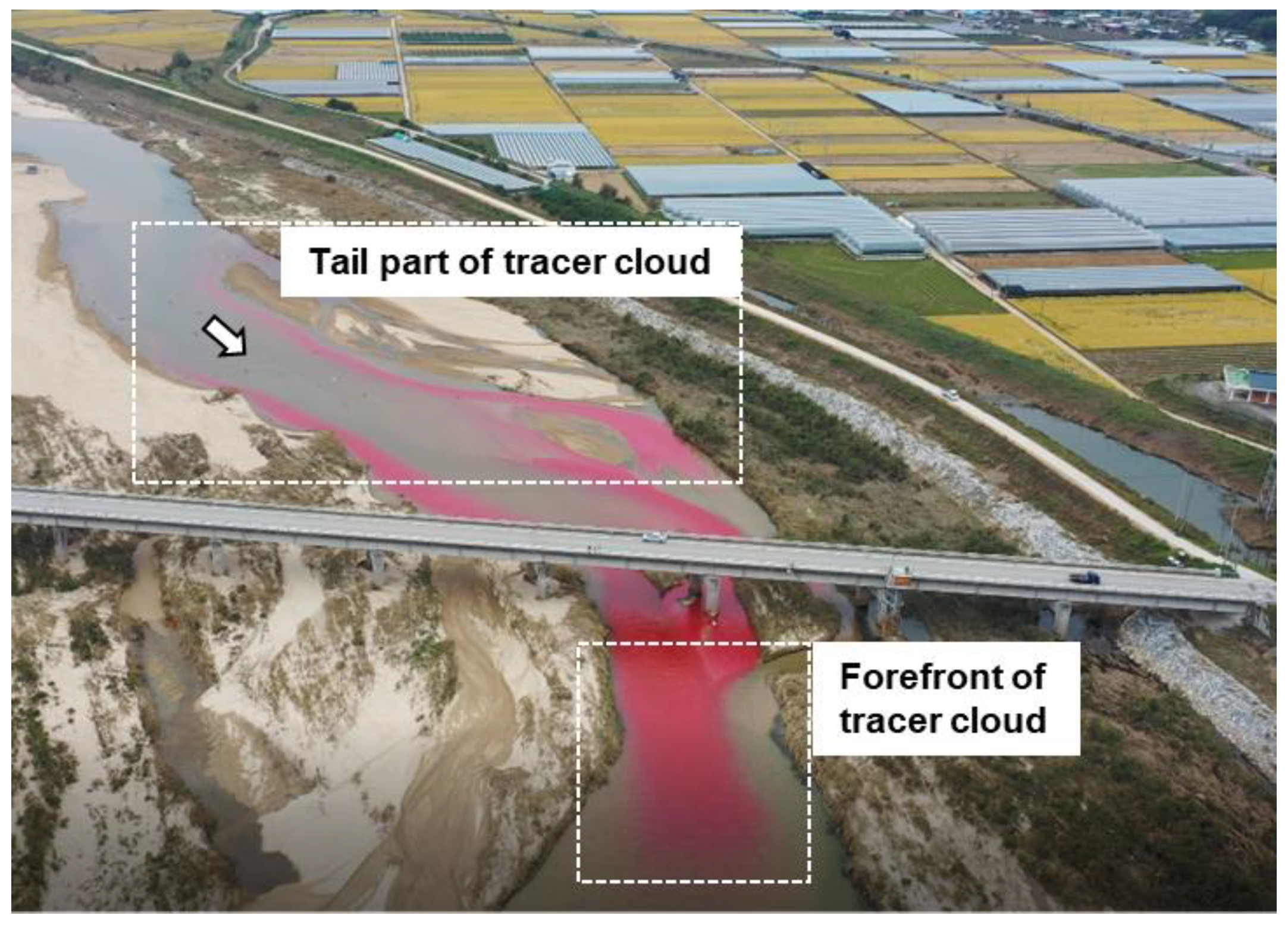
Solute transport models in natural streams enhance our understanding of contaminant transport and mixing, enabling us to respond effectively to chemical accidents and analyze biogeochemical cycling [1,2,3,4]. These models range from one-dimensional (1D) to three-dimensional (3D), with 1D modeling being particularly useful for predicting the fate of contaminants with low computational cost. In addition, their calibrated parameters provide valuable insights into the characteristics of fluvial systems. Classical 1D models, e.g., 1D advection-dispersion equation (ADE) [5], is fundamentally according to Fick’s law, which assumes the mixing behavior of passive scalars in streams as they are transported by the mean flow and dispersed by turbulence and shear velocities. However, in natural streams, solutes transport can be delayed by storage zones, such as eddies, pools, vegetation, artificial structures, and bed materials. This retention behavior often results in the distorted tracer cloud shape with a long tail (e.g., Figure 1), and the skewed concentration-time curve, called breakthrough curve [6,7]. In such occasions, an accurate prediction cannot be achieved by only adopting conventional Fickian approaches.

To account for these non-Fickian mixing events owing to the storage effect, numerous methods have been proposed, including a numerical model, a stochastic model, and an analytical approach [8,9,10,11,12]. For example, the transient storage model (TSM) conceptually incorporates the influence of storage zones by adding an additional sink-source term into the ADE [8,13]. Specifically, it deals with a river section by dividing it into two zones: the mainstream and storage zones, where the flow is very slow or stagnant. Linear mass exchange between the two zones was used to account for the storage effect [8]. The TSM describes the complex storage characteristics of natural rivers using the relative size of the storage area $ϵ$ and a single-rate solute exchange rate coefficient $\alpha$; the accuracy of the TSM significantly depends on these parameters [10]:

$$\frac{\partial \overline{c}}{\partial t}=-\overline{u}\frac{\partial \overline{c}}{\partial x}+\frac{\partial }{\partial x}\left(D_L\frac{\partial \overline{c}}{\partial x}\right)+\alpha \left({\overline{c}}_s-\overline{c}\right),$$

(1a)

$$\frac{\partial {\overline{c}}_s}{\partial t}=\frac{\alpha }{ϵ}\left(\overline{c}-{\overline{c}}_s\right),$$

(1b)

where $\overline{c}$ and ${\overline{c}}_s$ are the cross-sectional average concentrations in the flow and storage zones, respectively; $\overline{u}$ is the reach-average flow velocity; $D_L$ is the longitudinal dispersion coefficient; $x$ is the distance in the streamwise direction; and $t$ is the time variable. The transient parameters are often represented by the mean residence time $T_m$, defined by $T_m=ϵ/\alpha$. Nevertheless, because the TSM parameters cannot be directly measured, determining the proper parameters remains challenging [14]. Moreover, it has been reported that the exponential memory function of TSM often reproduces a poor tail distribution of trace breakthrough curves in natural rivers [4,15].

Subsequently, various conceptual models for non-Fickian solute transport in streams have been proposed. Deng et al. [16] proposed the fractional advection-dispersion equation (FADE) by expressing the variance term of the existing ADE in the form of F-order differentiation, and numerically modeled it by finding F-values that are similar to actual phenomena. Boano et al. [17] developed a continuous-time random walk (CTRW) model, which probabilistically models the distance that a solute moves in a river at random. Several researchers have proposed the solute transport in river (STIR) model, in which two different memory functions are applied to consider various residence time scales from surface storage zones to hyporheic exchange [18,19]. Other approaches, including the variable residence time model [20] and, the modified advection-dispersion equation [21], also attempt to find proper modeling to interpret the non-Fickian mixing. The primary goals in characterizing non-Fickian solute transport in streams are to improve accuracy by comprehensively accounting for various residence time scales and minimizing uncertainty in the associated parameters. Their formulae have a form of an implicit partial differential equation and are often numerically resolved by discretizing the spatio-temporal domain [22]. Little studies have suggested their explicit solutions, which is more deterministic and straightforward.

In this study, an exact and efficient solution for simulating concentration variations via non-Fickian transport is presented. A solution based on the Gaussian approximation for the shape-free boundary condition was derived using the routing procedure [20], and the storage effect was incorporated using the stochastic concept of [18]. Hence, an explicit formula for resolving non-Fickian transport was proposed, and the validity of the new formula was demonstrated by comparing it with analytical and numerical solutions of the transient storage model using synthetic data, and then its prediction accuracy was validated using a field data. Furthermore, the validated formula was used to interpret the tailing problem of the late-time behavior of the breakthrough curves.

2. Materials and Methods

2.1. Model Description

2.1.1. Formulation for Non-Fickian Tracer Transport

For an incompressible fluid, the mass-conservative Fick’s law implies that the transport of a passive scalar, which is any substance being transported that does not affect the flow of the media, is dominated by advection and diffusion, as shown in Equation (2):

$$\frac{\partial c}{\partial t}+u·\nabla c=\nabla ·\left(D\nabla c\right),$$

(2)

where $c\left(x,y,z,t\right)$ is the instantaneous concentration of the solute; $u=\left(u,v,w\right)$ is the velocity vector; and $D$ is the isotropic diffusion coefficient. In a riverine environment, because the shear effect from the advective velocity gradient significantly exceeds the molecular or turbulent diffusion effect [23], the diffusive property of $D$ is attributed to the dispersion effect; hence, $D$ here represents the dispersion coefficient. Unlike diffusion kinematics, the dispersion phenomenon cannot be considered isotropic as the velocity gradients in the vertical and transverse directions are greater than that in the longitudinal direction on account of the riverbed boundary. Consequently, after the precedence of the cross-sectional mixing, Equation (2) can be expressed as

$$\frac{\partial \overline{c}}{\partial t}+\overline{u}\frac{\partial \overline{c}}{\partial x}=D_L\frac{{\partial }^2\overline{c}}{\partial x^2}.$$

(3)

The analytical solutions for Equation (3), along with the restricted boundary conditions (for example, a continuous source with a constant concentration or an instantaneous source with a mass), were derived by [24]. However, these underlying premises are not feasible for actual streams. To derive a more practical formulation of the solution in which a shape-free breakthrough curve can be applied as an upstream boundary condition, the concept of a routing procedure was employed [25]. The routing procedure was initially developed [5] to predict the dispersion coefficient when the breakthrough curves at the upstream and downstream boundaries were known. In other words, the routing procedure can be used to predict the concentration at the downstream boundary from upstream boundary concentration. The formulation of the routing model with respect to the concentration variation over time is inferred as follows:

$$\overline{c}\left(t;x\right)={{\displaystyle \int }}_0^t\frac{\overline{c}\left(\tau ;0\right)\overline{u}}{\sqrt{4\pi D_L{T}_c}}\mathit{exp}\left|-\frac{{\left(x-\left(t-\tau \right)\overline{u}\right)}^2}{4D_L{T}_c}\right|d\tau ,$$

(4)

where $T_c$ is the characteristic advection time defined by $T_c=x/\overline{u}$. The derivation of the routing model is premised on the frozen cloud assumption that the tracer cloud hardly changes during the time required to pass the observation point. According to Equation (4), the variation in the breakthrough curve from $\overline{c}\left(t;0\right)$ to $\overline{c}\left(t;x\right)$ can be predicted once the parameters $\overline{u}$ and $D_L$ are determined.

Many studies have shown that the actual tracer transport does not follow Fickian transport. Tracer transport in a stream is derived not only by advection and dispersion but also by the additional delay effect, the so-called storage effect. The tracer cloud was partially trapped in the stagnant or low-flow zones and released back into the main flow after some residence time. Thus, non-Fickian transport can be characterized by quantifying the mean residence time, which is representative of the entire tracer cloud. Herein, the transfer function $\mathsf{\Phi }$ is incorporated into Equation (4) as

$$\overline{c}\left(t;x\right)={{\displaystyle \int }}_0^t{{\displaystyle \int }}_0^{\tau 2}\frac{\overline{c}\left({\tau }_1;0\right)\overline{u}}{\sqrt{4\pi D_L{T}_c}}\exp \left|-\frac{{\left(x-\left({\tau }_2-{\tau }_1\right)\overline{u}\right)}^2}{4D_L{T}_c}\right|\mathsf{\Phi }\left(t-{\tau }_2\right)d{\tau }_{1}d{\tau }_2.$$

(5)

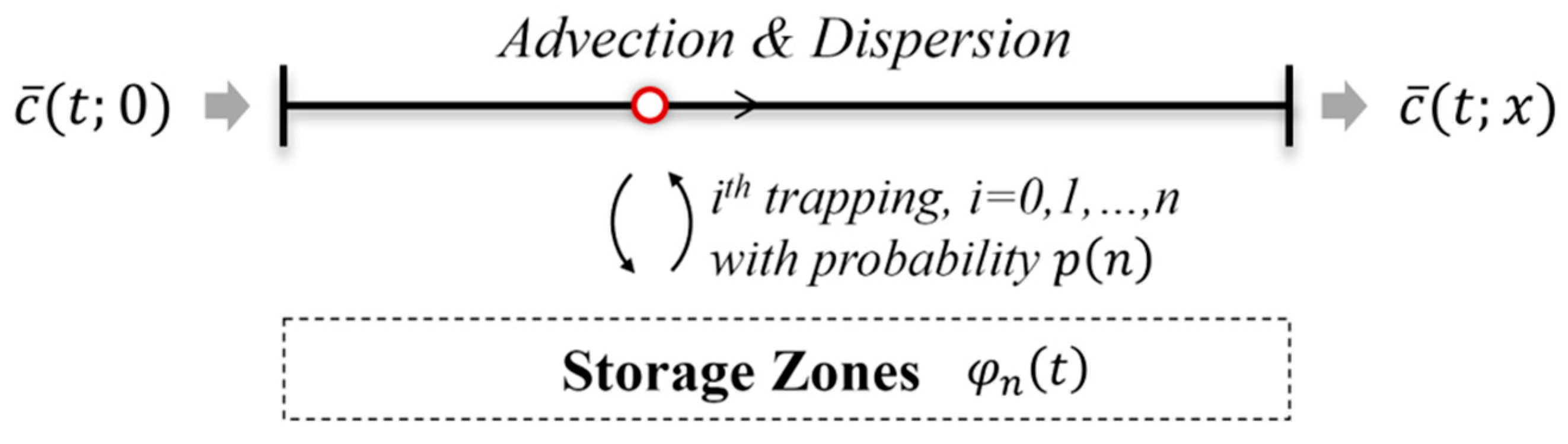
The transfer function $\mathsf{\Phi }$ is a function of time, and essentially ${\displaystyle \int }\mathsf{\Phi }dt=1$. The time variable in $\mathsf{\Phi }$ stands for the retention time so that $\mathsf{\Phi }$ is a kind of probability density function with respect to the net retention time. Therefore, finding a proper distribution or model for $\mathsf{\Phi }$ is the key to non-Fickian transport modeling [26]. In this study, the stochastic approach proposed in [18,19] was used to formulate the transfer function. The generic configuration of particle transport with trappings is shown in Figure 2. For a particle being transported along the streamflow, the net retention time can be estimated by the number of trapping events and the retention time at each trapping. Thus, the equation becomes

$$\mathsf{\Phi }\left(t\right)={\displaystyle \sum }_{n=0}^{\infty }p\left(n\right){\phi }_n\left(t\right),$$

(6)

where $p$ is the probability density function with respect to the trapping number, ${\phi }_n$ is the residence time distribution for $n$-times trapping, and $n$ is the number of occurrences. The trapping event can be interpreted as a finite sequence of random binary variables, the so-called Bernoulli process [27], assuming that the probability of the trapping event is identically distributed along the reach. Additionally, each trapping event is not affected by its history, that is, it occurs independently, which is a requirement of the Bernoulli process. In this respect, $p$ can be approximated using the Poisson distribution, when the average rate $\alpha$ is given, at which events occur, as

$$p\left(n\right)=\frac{{\left(\alpha T_c\right)}^n{e}^{-\alpha T_c}}{n!}.$$

(7)

Hence, the solution of Equation (5) can be rearranged as

$$\overline{c}\left(t;x\right)={{\displaystyle \int }}_0^t{{\displaystyle \int }}_0^{{\tau }_2}\frac{\overline{c}\left({\tau }_1;0\right)\overline{u}}{\sqrt{4\pi D_L{T}_c}}\exp \left|-\frac{{\left(x-\left({\tau }_2-{\tau }_1\right)\overline{u}\right)}^2}{4D_L{T}_c}\right|{\displaystyle \sum }_{n=1}^{\infty }\left(\frac{{\left(\alpha T_c\right)}^n{e}^{-\alpha T_c}}{n!}\right){\phi }_n\left(t-{\tau }_2\right)d{\tau }_{1}d{\tau }_2.$$

(8)

The proposed solution can explicitly compute the breakthrough curve at $x$ without segmenting reaches. Compared to the numerical solution of the implicit equation (e.g., [28]), this enables us to avoid potential numerical errors, resulting in a simpler and more accurate solution with a lower computational cost. But, the numerical error could still exist from the process of integrating the temporally discrete data $c\left(t;0\right)$, and truncating the infinite summation with increasing $n$.

The ${\phi }_n$ is the total residence time distribution when the trapping with $\phi$ occurs $n$-times. The superposition of two $\phi$ can be computed using the convolution operator, defined by $\phi \left(t\right)\ast \phi \left(t\right)\equiv {{\displaystyle \int }}_0^t\phi \left(\tau \right)\phi \left(t-\tau \right)d\tau$, so that ${\phi }_n$ is defined in which the n of $\phi$ were convolved. A variety of formulations for $\phi$ has been proposed, e.g., exponential distribution ${\phi }_e$ [29], log-normal distribution ${\phi }_l$ [4], power-law distribution ${\phi }_p$ [15,30], and advective pumping model ${\phi }_p$ [31]. Among them, ${\phi }_e$ and ${\phi }_p$ defined by

$${\phi }_e=\frac{1}{T_m}{e}^{-\frac{t}{T_m}},$$

(9)

$${\phi }_p=\frac{\frac{\pi }{T_m}}{10.66\frac{T_m}{t}+{\left(\frac{t}{T_m}+2\right)}^2}.$$

(10)

The proper distribution for $\phi$ can be selected according to the temporal- and spatial- scale of the retention effect of the field. In this study, two empirical formulas were applied to the proposed solution. When considering ${\phi }_e$, Equation (7) becomes equivalent to Equation (1). In this study, to verify the proposed formula, the analytical and numerical solutions of TSM, Equation (1), were also derived. According to the definition of $\phi$, a solution can be derived from the Laplace domain. The initial implicit formulation for the non-Fickian transport incorporating the $\phi$ can be inferred as

$$\frac{\partial }{\partial t}\overline{c}\left(t;x\right)=\left(-\overline{u}+D_L\frac{\partial }{\partial x}\right)\frac{\partial }{\partial x}\overline{c}\left(t;x\right)-\alpha \left(\overline{c}\left(t;x\right)-\overline{c}\left(t;x\right)\ast \phi \left(t\right)\right).$$

(11)

Equation (11) can be expressed in the Laplace domain as

$$\left[s+\alpha \left(1-\tilde{\phi }\left(s\right)\right)\right]\tilde{c}\left(s;x\right)+U\frac{\partial }{\partial x}\tilde{c}\left(s;x\right)-D_L\frac{{\partial }^2}{\partial x^2}\tilde{c}\left(s;x\right)=\tilde{c}\left(t=0\right),$$

(12)

where

$$\tilde{c}\left(s;x\right)={{\displaystyle \int }}_0^{\infty }{e}^{-st}\overline{c}dt,$$

(13)

where $s$ denotes a Laplace variable. The analytical solution for Equation (12) was derived following the work of [32] in the Laplace domain, resulting in

$$\tilde{c}\left(s;x\right)=\tilde{c}\left(s;0\right)\exp \left[\left(\frac{\overline{u}-\sqrt{{\overline{u}}^2-4D_L\left(\alpha \tilde{\phi }\left(s\right)-\alpha -s\right)}}{2D_L}\right)\right].$$

(14)

The boundary condition $\tilde{c}\left(s;0\right)$ was set as the Laplace-transformed Heaviside function, signifying that the tracer was introduced from time $t_1$ to $t_2$ at a constant concentration ${\overline{c}}_0$.

$$\tilde{c}\left(s;0\right)=\frac{{\overline{c}}_0}{s}\left(e^{-t_{1}s}-e^{t_{2}s}\right)$$

(15)

For the inversion of the Laplace transform, the precalculated approximation polynomials are normally suggested such as [33]. However, because the order of the polynomials cannot be easily increased in the inversion problem, a numerical inversion method based on the Bromwich integral was used to compute Equation (14) [34]. In this study, the numerical solution to Equation (1) was built following the work on the OTIS model [22].

2.1.2. Parameter Determination

Since the proposed solution includes the empirical parametric formulation for $\phi$, appropriate parameter determination is the key to the accuracy of the simulation. Herein, the optimal parameters were found in which the best fit of the breakthrough curve with minimum errors was simulated. Mean squared error (MSE) ${ϵ}_{MSE}$, which is a commonly-used metric to measure the quality of a model prediction, was used as a cost function for optimization, defined by

$${ϵ}_{MSE}=\frac{1}{N_{obs}}{{\displaystyle \sum }}_{j=1}^{N_{obs}}{\left({\overline{c}}_{obs}^j-{\overline{c}}_{sim}^j\right)}^2,$$

(16)

where ${\overline{c}}_{obs}^j$ and ${\overline{c}}_{sim}^j$ are the observed and simulated cross-sectional average tracer concentrations, respectively, at the jth time step, and $N_{obs}$ is the number of observations. The sequential least squares programming (SLSQP) scheme was used as a multivariate optimization scheme, in which the optimal parameters were determined using the quasi-Newton method [35]. The optimal set of the four model parameters; $\overline{u}$, $D_L$, ${\alpha }_t$, and $T_c,$ were concurrently calibrated within reasonable ranges to find the best-fit breakthrough curve with minimum ${ϵ}_{MSE}$.

2.2. Field Experiment

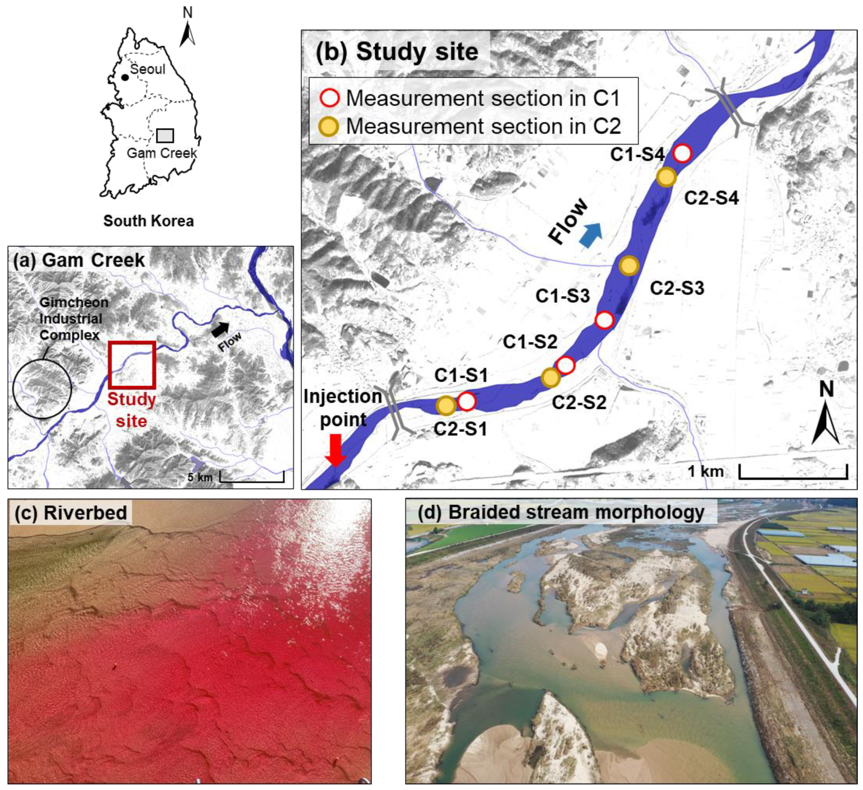
To acquire field data, tracer tests were conducted at Gam Creek, the first tributary of the Nakdong River, located across the cities of Gimcheon and Gumi in Gyeongsangbuk-do, South Korea, as shown in Figure 3. Gam Creek flows through a complex area of agricultural land, industrial complexes, and residential areas, and is a potentially high-risk area for hazardous chemical spills. Furthermore, as shown in Figure 3, the riverbed mainly consists of sand and has many complex braided flow sections, as shown in Figure 3c,d. Notably, sand dunes are formed in the entire section, which can increase the residence time of the solute owing to the dynamic interaction between the hyporheic zone and the main flow area [36,37,38]. The geomorphological features of Gam Creek indicate the existence of flow stagnation zones and the storage effect; additionally, this river has been used as an appropriate study site to verify the storage effect reproduced by the model, as detailed by Kim et al. [7].

In this study site, two tracer tests were conducted on 17 October 2019 and 4 June 2020, under different discharge conditions of 12.86 m³/s and 2.17 m³/s [7], respectively. The study site has a total reach length of 4.85 km, and is divided into three subreaches with measurement sections. The length of the subreaches ranged from 800 to 2000 m, as shown in Figure 3b. The hydraulic and geometric parameters of each subreach were estimated by averaging the measured values obtained in the upstream and downstream measurement sections, as listed in

Table 1. Hydraulic and geometric parameters of each sub-reach in the two tracer tests.

Case	Sub-Reach	Length (m)	Discharge (m3/s)	Velocity (m2/s)	Area (m2)	Width (m)	Depth (m)
C1	SR1 (C1-S1–C1-S2)	1200	12.63	0.610	20.69	57.36	0.361
	SR2 (C1-S2–C1-S3)	830		0.598	21.10	58.86	0.358
	SR3 (C1-S3–C1-S4)	2000		0.553	22.83	53.00	0.431
C2	SR1 (C2-S1–C1-S2)	954	2.17	0.322	6.17	20.75	0.305
	SR2 (C2-S2–C1-S3)	1798		0.317	6.06	15.45	0.388
	SR3 (C2-S3–C1-S4)	1105		0.315	6.74	16.75	0.395

. In the measurement sections, cross-sectional velocity and water depth were measured using an acoustic Doppler velocimeter (Sontek FlowTracker) with a velocity accuracy of ±0.001–4.0 m/s [39]. The location and width of the sections were measured using a real-time kinematic GPS (RTK-GPS) (Sokkia GRX1). Based on these sectional measurements, the velocity magnitude of each subreach was calculated by averaging the upstream and downstream sections. Furthermore, the bed slope ($S_0$) was calculated by dividing the bed elevation difference between the upstream and downstream sections by the sub-reach length.

The tracer was injected at multiple horizontal points to accelerate complete mixing in the transverse and vertical directions in the measurement sections. Moreover, the complete mixing distance ($L_c$) was calculated using Equation (17), as proposed by Kilpatrick and Wilson [40], to position the first sections farther than this distance.

$$L_c=0.1{\left(\frac{1}{n}\right)}^2\frac{U{W}^2}{{\epsilon }_t},$$

(17)

where $n$ is the number of horizontal injection points, $U$ is the mean velocity, $W$ is the width, and ${\epsilon }_t$ is the transverse mixing coefficient, which was calculated from ${\epsilon }_t/H{U}_{\ast }=0.15$ [24]. In this calculation, the shear velocity ($U_{\ast }$) was estimated as $U_{\ast }=\sqrt{gH{S}_0}$. Consequently, the injection point for the tracer was set approximately 700 m upstream of the first sections (C1-S1 and C2-S1) for both tests (Figure 3b).

The fluorescent tracer Rhodamine WT was used because of its high visibility and conservative characteristics as a passive scalar [41]. To measure the downstream breakthrough curves of the tracer, three to four YSI-600OMS sensors were deployed at each measurement section. These sensors have an accuracy of ±5% or 1 ppb error and can measure concentrations in the range of 0 to 200 ppb. Prior to the tracer test, the sensors were calibrated using standard solutions of known concentrations within the measurable range, and the sampling rate of all sensors was set to 4 s. To prevent the concentration from exceeding the measurable range, 20 L of 2000 ppb Rhodamine WT were injected for the tracer test. The measured breakthrough curves at several points at each section were averaged to obtain the 1D breakthrough curves, and a moving-average filter was used to smooth the breakthrough curves. The detailed datasets observed in both experiments are available in [7].

3. Results and Discussion

3.1. Verification by Synthetic Data

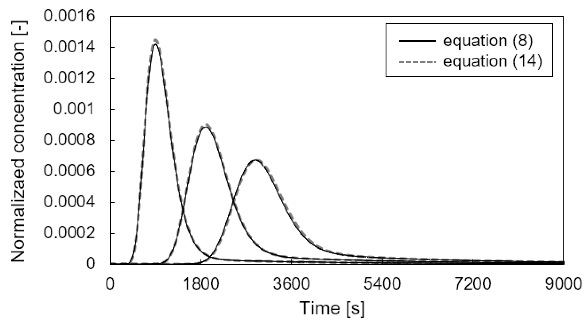
To verify the proposed formula, Equation (8), its simulation was compared with that of the analytical solution of Equation (14) under identical conditions. For both, the exponential equation was employed for the empirical parametric formulation for $\phi$. Given the assumptions of Equation (14) including the Heaviside input function, a scenario was set up: a conservative passive tracer with ${\overline{c}}_0$ initial concentration is introduced at the upstream boundary of a prismatic channel for 30 s, and its breakthrough curves at 500, 1000, and 1500 m downstream of the inlet were predicted. The parameters related to the flow condition; $\overline{u}$, $D_L$, $T_m$, and $\alpha$, were configured as 10 m/s, 5 m²/s, 250 s, and 0.001 s⁻¹, respectively, which are typical values of each parameter. A comparison of the results from both equations demonstrates their equivalence, with a determination coefficient (R²) of over 0.99 (see Figure 4). The slight differences between them are attributed to the discrete $\overline{c}\left(t;0\right)$ input and the operation of multiconvolution in Equation (8).

In addition, the results of the proposed formula were compared with the numerical solution of Equation (1) to emphasize the advantage of the analytical approach over numerical analysis. Because the numerical approach resolves the implicit Equation (1) by segmenting the spatial domain with a grid size, its computation result is dependent on the grid size. Figure 5a shows a breakthrough curve comparison; undesired numerical diffusion and numerical oscillation were observed owing to the large grid size. Figure 5b shows that the numerical solution required almost nine times the computation time to yield a result that was as exact as the proposed formula. It may require less computation time than the proposed model when the grid size is large, but cannot yield exact results.

3.2. Validation by Field Data

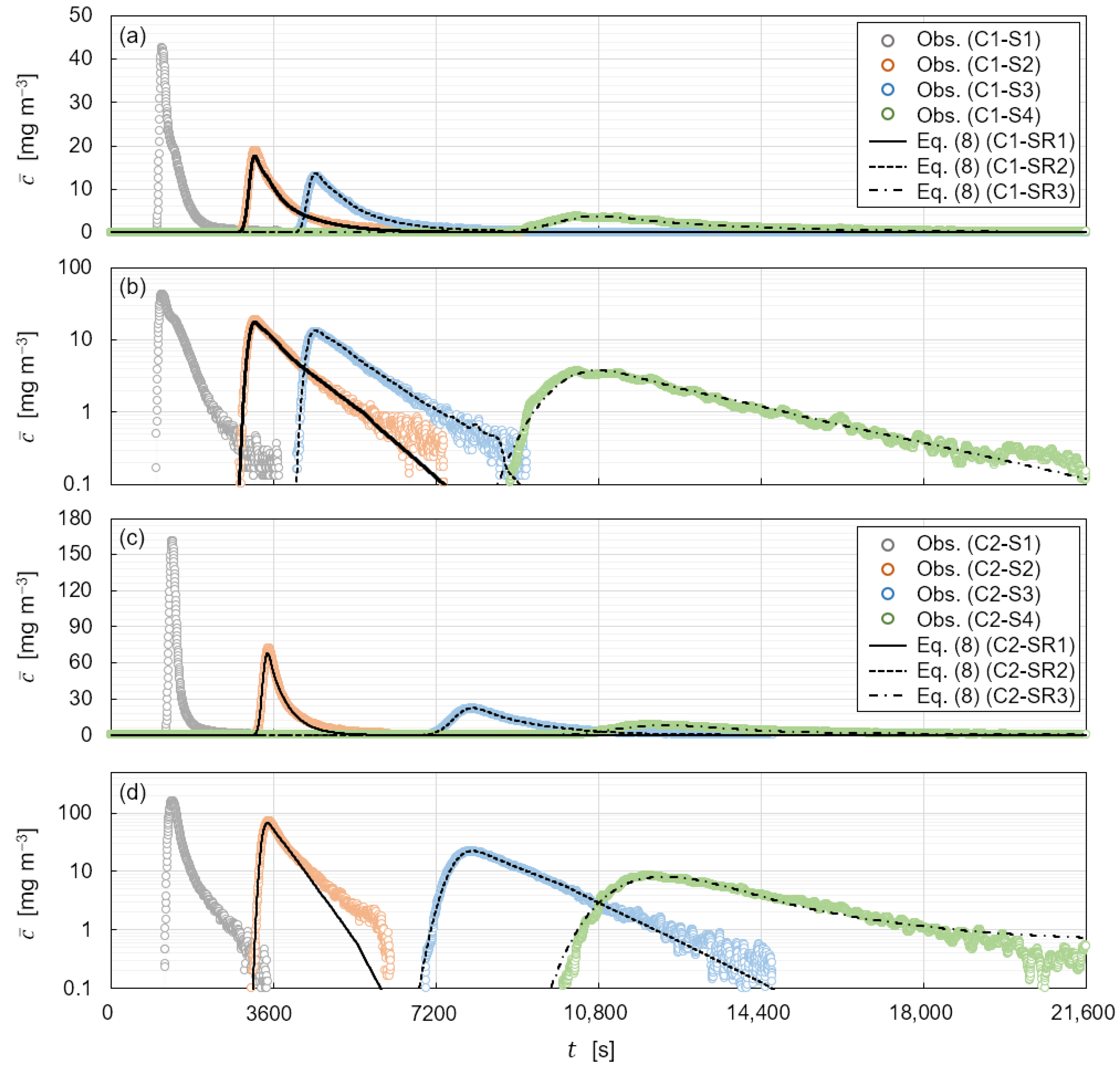
In this section, the proposed formula is used to simulate tracer transport in actual streams. Simulations were conducted along six subreaches corresponding to the acquired field datasets. The observed breakthrough curves were applied for $\overline{c}\left(t;0\right)$ at the inlet boundaries of each subreach. The optimal values for the empirical parameters of the solution relevant to the flow characteristics of each subreach were determined, and are listed in

Table 2. Calibrated parameters for each case.

Simulation Case	$\overline{\mathit{u}}$ (m)	${\mathit{D}}_{\mathit{L}}$ (m2·s−1)	${\mathit{T}}_{\mathit{m}}$ (s)	$\mathit{\alpha }$ (10−4·s−1)
C1-SR1	0.605	0.56	604.94	3.76
C1-SR2	0.644	0.59	536.39	2.92
C1-SR3	0.355	4.89	2187.74	1.54
C2-SR1	0.465	0.17	201.39	5.57
C2-SR2	0.420	1.73	827.86	2.01
C2-SR3	0.315	6.94	5767.09	1.35

. Despite the significant difference in the flow rates between C1 and C2, both revealed the largest $D_L$ and $T_m$ in SR3. Because $D_L$ accelerates the Gaussian dispersion and $T_m$ enhances the tailing effect, SR3 is the most mixing-inducing environment among the subreaches, which is attributed to its highly braided channel geometry, as seen in Figure 3d.

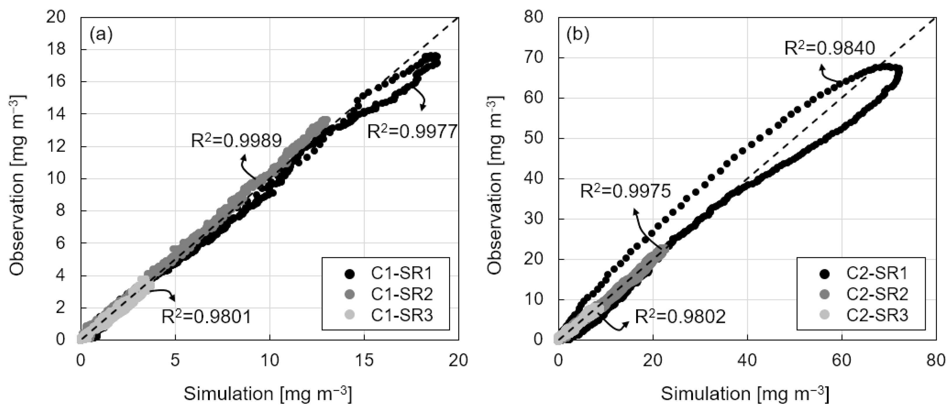
In each case, a parameter-calibrated equation was used to compute the breakthrough curve downstream of the boundary. The validity of the simulated non-Fickian tracer transport was demonstrated by comparing it with the observed breakthrough curves, as plotted in Figure 6. In the two cases of the tracer test, distinct breakthrough curves were observed on account of the differences in discharge and morphological changes between the two tests conducted at different times. The breakthrough curves in C1 advected faster than those in C2 because of the higher velocity and discharge, whereas the breakthrough curves for C2 were more dispersed, as indicated by the higher calibrated $D_L$ in Table 2. Furthermore, the breakthrough curves in both cases exhibit a notably skewed and long-tailed shape, implying a high storage zone effect resulting from the complex braided geometry or the hyporheic zone. The tailing parts of the curves in both cases also show different shapes, as demonstrated by the log-transformed curves in Figure 6b,d. This figure indicates that the tailing parts of both curves followed a power-law form, as reported in previous studies [42,43]. However, the slopes of the tails differed owing to the varying storage zone effect. In other words, interpreting the tails of breakthrough curves can provide information about the stream. Despite this potential, the tailing part contained relatively high noise, because the lower sensing limit of the YSI sensor is highly sensitive to interference from the optical scattering of suspended matter or turbulence. The noise increased downstream toward the reach as the overall concentration decreased. As is evident from these observed data, the breakthrough curves entail the complex flow and mixing characteristics of the stream, as well as high noise. Therefore, a more precise model is essential to interpret such non-Fickian phenomena from breakthrough curves.

Despite the highly skewed observed breakthrough curves, the overall accuracy of all cases was substantial, with an average deterministic coefficient (R²) of 0.990 (Figure 7). In addition to the main body of the tracer cloud around the peak, the tailing was well reproduced. In conclusion, the explicit formula proposed in this study is an efficient and effective alternative for simulating non-Fickian tracer transport once appropriate parameters are determined. Nonetheless, as shown in Figure 6, in some cases, the simulation results along the tailings did not closely follow the attenuation of the observed tracer concentration. This will be discussed further in the next section.

3.3. Late-Time Behavior of the Breakthrough Curve

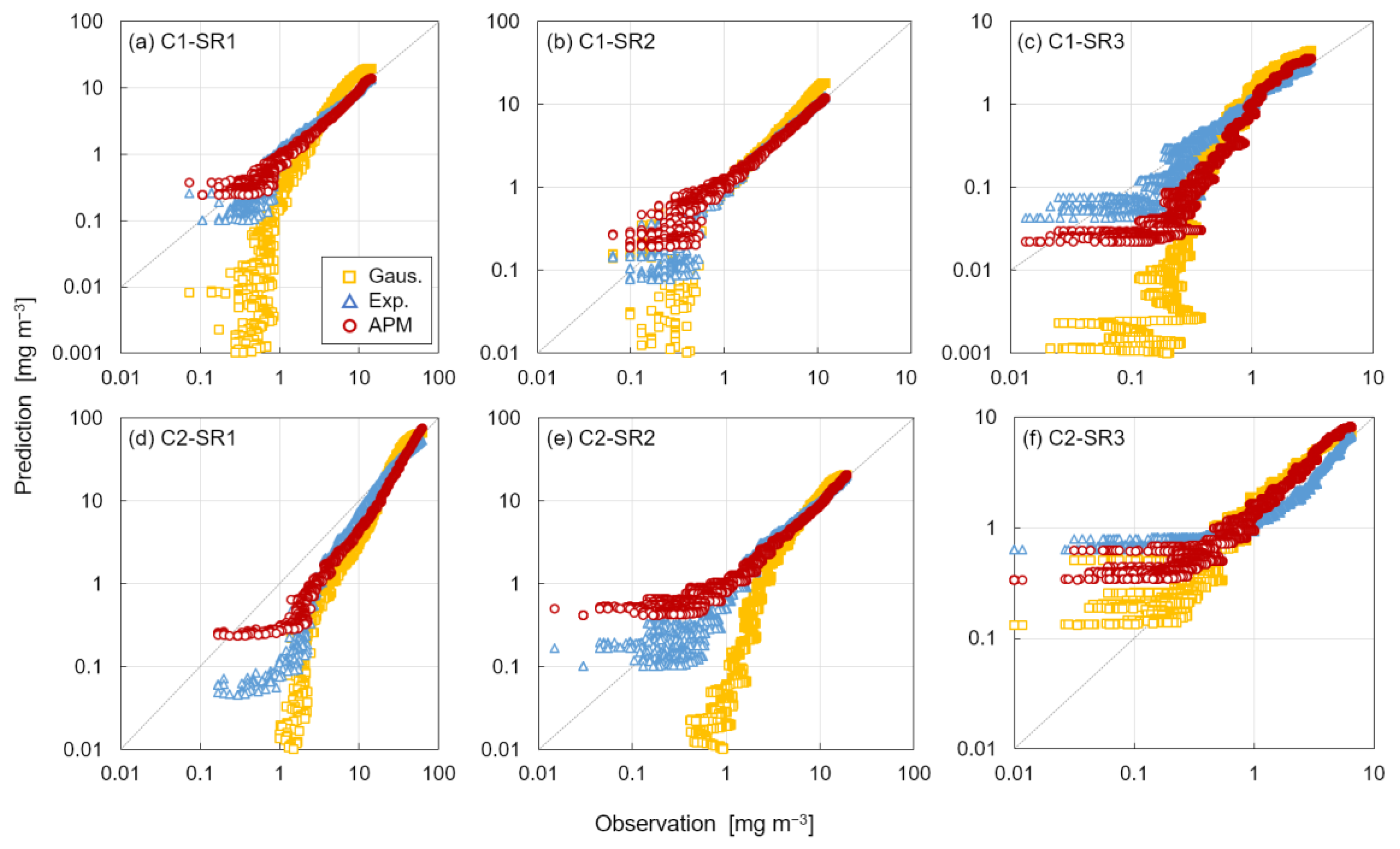
The late-time behavior of breakthrough curves is often crucial for interpreting the deposition and accumulation of pollutants. It was previously observed that simulations mostly underestimated the tailing effect. This aspect has already been found by, e.g., [44,45,46], and is commonly attributed to the memory function $\phi$. Due to the exponential ${\phi }_e$ so far applied, the tracer concentration was more rapidly attenuated than the actual tracer, except for C2-SR3. This corresponds to the arguments of existing studies (e.g., [16,33,47]), saying that the exponential memory function is suitable for short residence time cases. As an alternative, ${\phi }_p$ was also applied, which approximates the exact solution of the advective pumping model. With the optimal parameters, it simulated the breakthrough curves, and the results were compared to those with ${\phi }_e$ and Gaussian approximations. To closely investigate the late-time behavior of the breakthrough curves, only the falling limb of the breakthrough curves is plotted on a log-log scale, as shown in Figure 8. All cases consistently show that the Gaussian approximation cannot reproduce the tailing effect in the 1D transport analysis. In other words, these results emphasize the necessity of non-Fickian transport modeling.

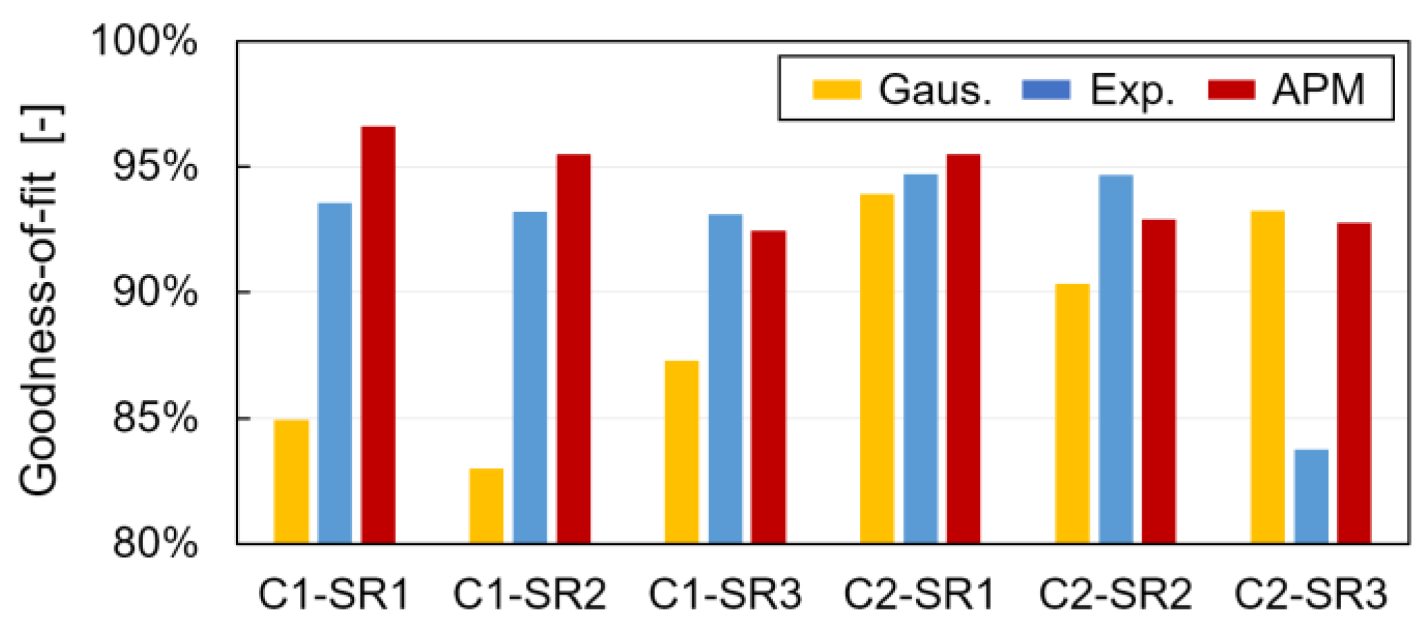
The simulation results of Equation (8) were compared in terms of goodness-of-fit, evaluated using the percentage log-scaled R² only for the tails (see Figure 9). The results with ${\phi }_p$ average outperformed those with ${\phi }_e$ in C1-SR1, C1-SR2, C2-SR1 by enhancing the tailing effect. These results correspond to those in [18], who verified the use of the advective pumping model. However, in C2-SR2 and C2-SR3, the tailing effects by ${\phi }_p$ were somewhat overestimated. In particular, in C2-SR3, all simulations overestimated the observed tails. This is seemingly because the tracer cloud was diluted with O(10 ppb) at the peak concentration and exhibited excessive variance. In these cases, finding proper parameters to distinguish the influence of the dispersion and tailing effects can be difficult, and simulated breakthrough curves can easily be heavy-tailed compared to actual tracer tails. Especially, the ${\phi }_e$ for C2-SR3 has 5767.09 s of $T_m$ which is appreciably large despite the relatively large $D_L$. In this case, the Gaussian approximation exhibited the best-fit tailing, indicating that the memory function is unnecessary. Overall, the suitability of the distribution for the memory function is likely to be data-dependent, i.e., the comparative advantage between ${\phi }_e$ and ${\phi }_p$ is unclear in these cases. Following the work of [18], using both could be a proper way to reproduce a better-fitting breakthrough curve, as long as a precaution on the overfitting problem is taken, inducing less generality.

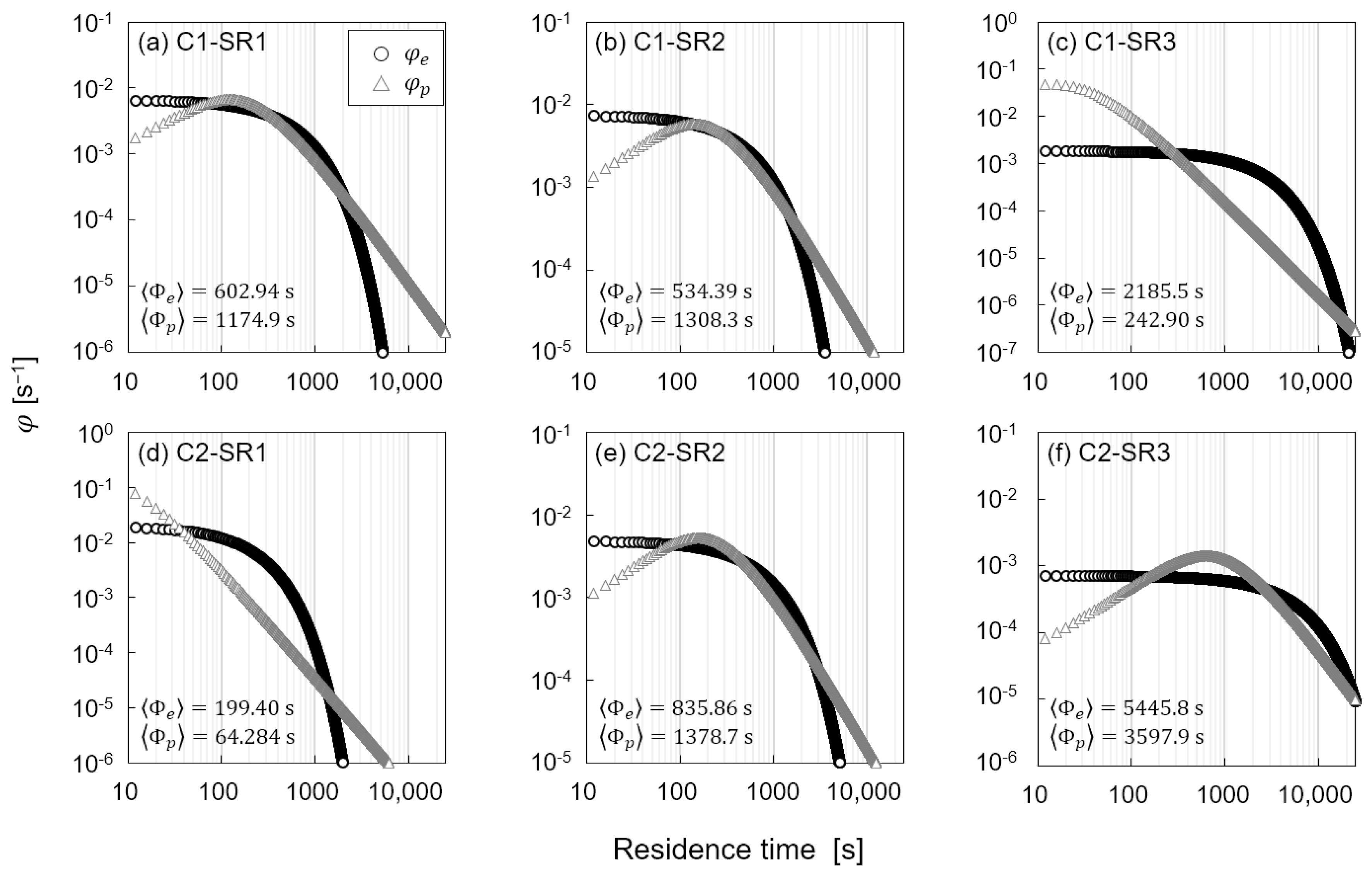
The determined optimal memory functions ${\phi }_e$ and ${\phi }_p$ were also compared in Figure 10. The behavior of the distributions representing the probability density function with respect to residence time was significantly different. Their expectations correspond to the parameter $T_m$ but are slightly different due to truncation errors. In terms of the ability of the memory function to consider a wider range of residence time, ${\phi }_p$ outperformed ${\phi }_e$. In other words, ${\phi }_p$ can consider the larger residence time scale that generates the longer tails, as shown in Figure 10. This aspect is important when considering the long-term residence time in, e.g., hyporheic zones, for which the exponential memory function may not be appropriate. However, in the SR3 of both cases, ${\phi }_e$ was more weighted to the larger time scale than ${\phi }_p$, because ${\phi }_p$ becomes equivalent to a power law distribution ${\phi }_p~\pi T_m{t}^{-2}$ when $t\to \infty$ [18]. In these cases, the heavier tailing is showed with ${\phi }_e$.

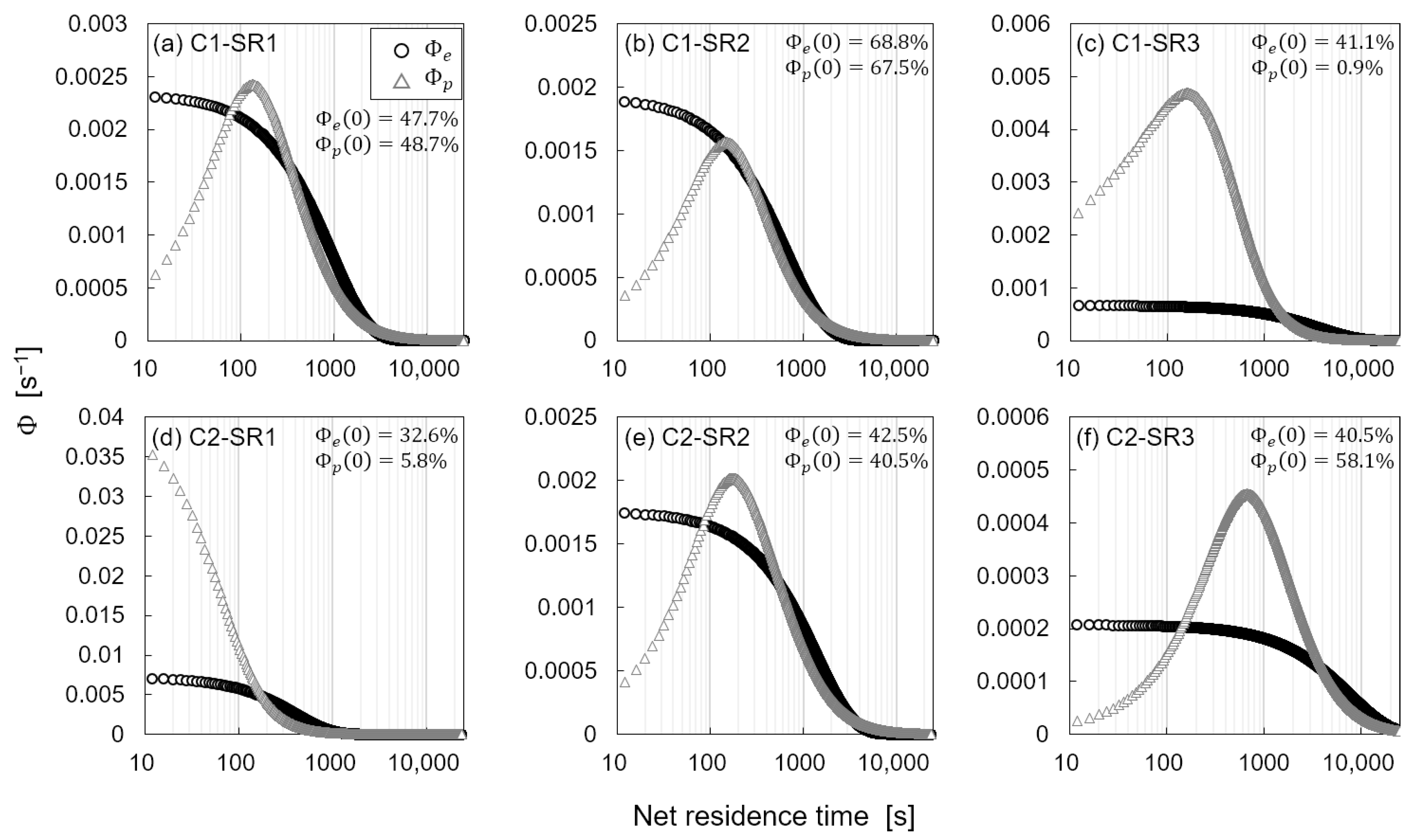
Note that the tailing effect is reproduced not only by the memory function, but also by $p\left(n\right)$ according to Equation (7). Therefore, the net retention time function $\mathsf{\Phi }$, in which those two functions are combined by Equation (5), were also compared in Figure 11. What is noteworthy is that the $\mathsf{\Phi }$ function has values at $t=0$. It is because of the zero-contribution of the $p$. Given that $\mathsf{\Phi }$ represents the net residence time in the stagnant zone, for which the tracer particles are stopped during the whole transport time in the sub-reach, $\mathsf{\Phi }\left(t=0\right)$ indicates the portion of the tracer that was not affected by the streambed boundary. This parameter represents the manner in which a given stream reaches a non-Fickian transport-inducing environment. In comparison to the net residence time scale, these are dependent not only on the subreach, but also on the shape of the memory function. For example, in C1-SR2, $\mathsf{\Phi }\left(t=0\right)$ is similar, but ${\mathsf{\Phi }}_e$ has more contribution of much smaller residence time scale according to its distribution. Basically, the ${\mathsf{\Phi }}_e$ has a shape that has maximum contribution at $t=0$, and gradually attenuates as net residence time increases. As the tracer transport is more delayed, i.e., the more temporal gap between flow velocity and tracer advective velocity occurs, the $\mathsf{\Phi }$ is shifted toward a larger net residence time scale. In this respect, the ${\mathsf{\Phi }}_e$ could not be proper to reproduce the net residence time of the tracer. This supports the results of previous studies, which maintained the discrepancy between the exponential memory function and tracer behavior in streams. In this respect, ${\mathsf{\Phi }}_p$ is more compatible for a wide range of residence time scale.

More importantly, significant differences in the late-time behavior of the breakthrough curves between the simulations and observations were generated at less than O(1 mg/m³). This concentration range is error-prone because the fluorescence-acquired data become excessively sensitive to other unknown influences, such as turbulence. These errors can negatively affect the optimization problem. The inconsistent results in determining the best distribution for the memory function can be attributed to dependence on the data and parameters. Even though it is commonly stated that ${\phi }_e$ is less proper for large residence time cases, a better result in simulating the breakthrough curve tail was shown in C2-SR3 case, by applying relatively large $T_m$. In other words, devising globally appropriate models for memory functions is challenging owing to data dependence. Nonetheless, the proposed formula required specifying the parametric memory function for operation, which remains an unsolved problem. It is more important to identify the true memory function from tracer data, for example, by employing deconvolution techniques [48], than to suggest memory function models by fitting the breakthrough curves.

4. Conclusions

In this study, an efficient solution was presented for predicting breakthrough curves in streams. The following conclusions were made:

• The proposed formula was validated by comparison with analytical and numerical solutions, and the results were exact. Its performance in simulating non-Fickian transport in streams was also validatesd using field tracer data, and good agreement was achieved.
• Despite the accurate results of reproducing the overall breakthrough curves, significant differences in their late-time behaviors were found according to the memory function modeling. This indicates that the best-fit breakthrough curve does not imply the accurate storage effect modeling.
• The tailing effect was discussed by comparing the optimal memory functions and net residence time functions. The key role of residence time-dependent functions is to enable us to quantitatively identify the storage effect, which is fundamental for a deeper understanding of non-Fickian tracer transport in streams. Hence, insight in characterizing non-Fickian mixing in can be provided from the memory function modeling.
• According to the data and optimal parameters, the proper formula for the memory function was inconsistent. The exponential memory function had a structural limit in generating a heavy-tailed breakthrough curve.

The proposed formula requires specifying the parametric memory function for operation, which remains an unsolved problem. Therefore, our next goal is to identify the true memory function from tracer data using deconvolution techniques rather than finding the best-fitting models for the breakthrough curves.

References

- Park, I.; Seo, I.W. Modeling Non-Fickian Pollutant Mixing in Open Channel Flows Using Two-Dimensional Particle Dispersion Model. Adv. Water Resour. 2018, 111, 105–120. [Google Scholar] [CrossRef]
- Seo, I.W.; Choi, H.J.; Do Kim, Y.; Han, E.J. Analysis of Two-Dimensional Mixing in Natural Streams Based on Transient Tracer Tests. J. Hydraul. Eng. 2016, 142, 04016020. [Google Scholar] [CrossRef]
- Kim, B.; Seo, I.W.; Kwon, S.; Jung, S.H.; Choi, Y. Modelling One-Dimensional Reactive Transport of Toxic Contaminants in Natural Rivers. Environ. Model. Softw. 2021, 137, 104971. [Google Scholar] [CrossRef]
- Wörman, A.; Wachniew, P. Reach Scale and Evaluation Methods as Limitations for Transient Storage Properties in Streams and Rivers. Water Resour. Res. 2007, 43. [Google Scholar] [CrossRef]
- Fischer, H.B. Dispersion Predictions in Natural Streams. J. Sanit. Eng. Div. 1968, 94, 927–943. [Google Scholar] [CrossRef]
- Kwon, S.; Noh, H.; Seo, I.W.; Jung, S.H.; Baek, D. Identification Framework of Contaminant Spill in Rivers Using Machine Learning with Breakthrough Curve Analysisremote Sensing. Int. J. Environ. Res. Public Health 2021, 18, 1023. [Google Scholar] [CrossRef]
- Kim, B.; Kwon, S.; Noh, H.; Seo, I.W. Surrogate Prediction of the Breakthrough Curve of Solute Transport in Rivers Using Its Reach Length Dependence. J. Contam. Hydrol. 2022, 249, 104024. [Google Scholar] [CrossRef]
- Bencala, K.E.; Walters, R.A. Simulation of Solute Transport in a Mountain Pool-and-Riffle Stream: A Transient Storage Model. Water Resour. Res. 1983, 19, 718–724. [Google Scholar] [CrossRef]
- Szeftel, P.; Dan Moore, R.D.; Weiler, M. Influence of Distributed Flow Losses and Gains on the Estimation of Transient Storage Parameters from Stream Tracer Experiments. J. Hydrol. 2011, 396, 277–291. [Google Scholar] [CrossRef]
- Noh, H.; Kwon, S.; Seo, I.W.; Baek, D.; Jung, S.H. Multi-Gene Genetic Programming Regression Model for Prediction of Transient Storage Model Parameters in Natural Rivers. Water 2021, 13, 76. [Google Scholar] [CrossRef]
- Marion, A.; Bellinello, M.; Guymer, I.; Packman, A. Effect of Bed Form Geometry on the Penetration of Nonreactive Solutes into a Streambed. Water Resour. Res. 2002, 38, 1209. [Google Scholar] [CrossRef]
- Kim, J.S.; Seo, I.W.; Baek, D.; Kang, P.K. Recirculating Flow-Induced Anomalous Transport in Meandering Open-Channel Flows. Adv. Water Resour. 2020, 141, 103603. [Google Scholar] [CrossRef]
- Thackston, E.L.; Schnelle, K.B.J. Predicting Effects of Dead Zones on Stream Mixing. J. Sanit. Eng. Div. 1970, 96, 319–331. [Google Scholar] [CrossRef]
- Choi, S.Y.; Seo, I.W.; Kim, Y.O. Parameter Uncertainty Estimation of Transient Storage Model Using Bayesian Inference with Formal Likelihood Based on Breakthrough Curve Segmentation. Environ. Model. Softw. 2020, 123, 104558. [Google Scholar] [CrossRef]
- Haggerty, R.; Wondzell, S.M.; Johnson, M.A. Power-Law Residence Time Distribution in the Hyporheic Zone of a 2nd-Order Mountain Stream. Geophys. Res. Lett. 2002, 29, 1640. [Google Scholar] [CrossRef] [Green Version]
- Deng, Z.; Singh, V.P.; Bengtsson, L. Numerical Solution of Fractional Order Advection-Reaction-Diffusion Equation. J. Hydraul. Eng. 2004, 130, 422–431. [Google Scholar] [CrossRef] [Green Version]
- Boano, F.; Packman, A.I.; Cortis, A.; Revelli, R.; Ridolfi, L. A Continuous Time Random Walk Approach to the Stream Transport of Solutes. Water Resour. Res. 2007, 43, 1–12. [Google Scholar] [CrossRef]
- Marion, A.; Zaramella, M.; Bottacin-Busolin, A. Solute Transport in Rivers with Multiple Storage Zones: The STIR Model. Water Resour. Res. 2008, 44. [Google Scholar] [CrossRef] [Green Version]
- Marion, A.; Zaramella, M. A Residence Time Model for Stream-Subsurface Exchange of Contaminants. Acta Geophys. Pol. 2005, 53, 527–538. [Google Scholar]
- Deng, Z.Q.; Jung, H.S. Variable Residence Time-Based Model for Solute Transport in Streams. Water Resour. Res. 2009, 45. [Google Scholar] [CrossRef]
- Singh, S.K. Treatment of Stagnant Zones in Riverine Advection-Dispersion. J. Hydraul. Eng. 2003, 129, 470–473. [Google Scholar] [CrossRef]
- Runkel, R.L.; Broshears, R.E. One-Dimensional Transport with Inflow and Storage (OTIS): A Solute Transport Model for Small Streams; Center for Advanced Decision Support for Water and Environmental Systems, Department of Civil Engineering, University of Colorado: Boulder, CO, USA, 1991. [Google Scholar]
- Absi, R. Reinvestigating the Parabolic-shaped Eddy Viscosity Profile for Free Surface Flows. Hydrology 2021, 8, 126. [Google Scholar] [CrossRef]
- Fischer, H.B.; List, E.J.; Koh, R.C.Y.; Imberger, J.; Brooks, N.H. Mixing in Inland and Coastal Waters; Academic Press: Cambridge, MA, USA, 1979. [Google Scholar]
- Baek, K.O.; Seo, I.W. Routing Procedures for Observed Dispersion Coefficients in Two-Dimensional River Mixing. Adv. Water Resour. 2010, 33, 1551–1559. [Google Scholar] [CrossRef]
- Kim, B.; Seo, I.W. Net Retention Time Distribution Inducing Non-Fickian Solute Transport in Streams. In Proceedings of the 39th IAHR World Congress, Granada, Spain, 19–24 June 2022. [Google Scholar]
- Dekking, F.M.; Kraaikamp, C.; Lopuhaa, H.P.; Meester, L.E. A Modern Introduction to Probability and Statistics; Springer: London, UK, 2005; Volume 157, ISBN 9781852338961. [Google Scholar]
- Runkel, R.L. One-Dimensional Transport with Inflow and Storage (OTIS): A Solute Transport Model for Streams and Rivers; US Department of the Interior, US Geological Survey: Reston, VA, USA, 1998; Volume 98.
- Bencala, K.E. Simulation of Solute Transport in a Mountain Pool-and-Riffle Stream With a Kinetic Mass Transfer Model for Sorption. Water Resour. Res. 1983, 19, 732–738. [Google Scholar] [CrossRef]
- Cardenas, M.B. Potential Contribution of Topography-Driven Regional Groundwater Flow to Fractal Stream Chemistry: Residence Time Distribution Analysis of Tóth Flow. Geophys. Res. Lett. 2007, 34. [Google Scholar] [CrossRef]
- Elliott, A.H.; Brooks, N.H. Transfer of Nonsorbing Solutes to a Streambed with Bed Forms: Theory. Water Resour. Res. 1997, 33, 123–136. [Google Scholar] [CrossRef]
- Kazezyilmaz-Alhan, C.M. Analytical Solutions for Contaminant Transport in Streams. J. Hydrol. 2008, 348, 524–534. [Google Scholar] [CrossRef]
- Polyanin, A.; Manzhirov, A. Handbook of Integral Equations; CRC Press: Boca Raton, FL, USA, 2008; pp. 961–968. [Google Scholar]
- Valsa, J.; Brančik, L. Approximate Formulae for Numerical Inversion of Laplace Transforms. Int. J. Numer. Model. Electron. Netw. Devices Fields 1998, 11, 153–166. [Google Scholar] [CrossRef]
- Kraft, D. A Software Package for Sequential Quadratic Programming; DFVLR: San Bruno, CA, USA, 1988. [Google Scholar]
- Yuill, B.; Wang, Y.; Allison, M.; Meselhe, E.; Esposito, C. Sand Settling through Bedform-Generated Turbulence in Rivers. Earth Surf. Process. Landf. 2020, 45, 3231–3249. [Google Scholar] [CrossRef]
- Kim, J.S.; Kang, P.K. Anomalous Transport through Free-Flow-Porous Media Interface: Pore-Scale Simulation and Predictive Modeling. Adv. Water Resour. 2020, 135, 103467. [Google Scholar] [CrossRef]
- Kim, J.S.; Kang, P.K.; He, S.; Shen, L.; Kumar, S.S.; Hong, J.; Seo, I.W. Pore-Scale Flow Effects on Solute Transport in Turbulent Channel Flows Over Porous Media. Transp. Porous Media 2023, 146, 223–248. [Google Scholar] [CrossRef]
- SonTek, SonTek FlowTracker2 Handheld-ADV Specifications. Available online: https://www.ysi.com/flowtracker2 (accessed on 28 March 2023).
- Kilpatrick, F.A.; Wilson, J.F. Measurement of Time of Travel in Streams by Dye Tracing; US Government Printing Office: Washington, DC, USA, 1989.
- Baek, D.; Seo, I.W.; Kim, J.S.; Nelson, J.M. UAV-Based Measurements of Spatio-Temporal Concentration Distributions of Fluorescent Tracers in Open Channel Flows. Adv. Water Resour. 2019, 127, 76–88. [Google Scholar] [CrossRef]
- Bayani Cardenas, M.; Wilson, J.L.; Haggerty, R. Residence Time of Bedform-Driven Hyporheic Exchange. Adv. Water Resour. 2008, 31, 1382–1386. [Google Scholar] [CrossRef]
- Aquino, T.; Aubeneau, A.; Bolster, D. Peak and Tail Scaling of Breakthrough Curves in Hydrologic Tracer Tests. Adv. Water Resour. 2015, 78. [Google Scholar] [CrossRef]
- Haggerty, R.; McKenna, S.A.; Meigs, L.C. On the Late-Time Behavior of Tracer Test Breakthrough Curves. Water Resour. Res. 2000, 36, 3467–3479. [Google Scholar] [CrossRef] [Green Version]
- Scott, D.T.; Gooseff, M.N.; Bencala, K.E.; Runkel, R.L. Automated Calibration of a Stream Solute Transport Model: Implications for Interpretation of Biogeochemical Parameters. J. N. Am. Benthol. Soc. 2003, 22, 492–510. [Google Scholar] [CrossRef] [Green Version]
- Kim, B.; Seo, I.W.; Kwon, S.; Jung, S.H.; Yun, S.H. Analysis of Solute Transport in Rivers Using a Stochastic Storage Model. J. Korea Water Resour. Assoc. 2021, 54, 335–345. [Google Scholar] [CrossRef]
- Drummond, J.D.; Covino, T.P.; Aubeneau, A.F.; Leong, D.; Patil, S.; Schumer, R.; Packman, A.I. Effects of Solute Breakthrough Curve Tail Truncation on Residence Time Estimates: A Synthesis of Solute Tracer Injection Studies. J. Geophys. Res. Biogeosci. 2012, 117. [Google Scholar] [CrossRef] [Green Version]
- Gooseff, M.N.; Benson, D.A.; Briggs, M.A.; Weaver, M.; Wollheim, W.; Peterson, B.; Hopkinson, C.S. Residence Time Distributions in Surface Transient Storage Zones in Streams: Estimation via Signal Deconvolution. Water Resour. Res. 2011, 47. [Google Scholar] [CrossRef] [Green Version]
Figure 1.
Skewed distribution of tracer cloud photographed at Gam Creek, South Korea (2019). The arrow indicates the flow direction.
Figure 2.
Schematic diagram of non-Fickian transport conceptualization.
Figure 3.
Overview of the tracer test in Gam Greek: (a) location of Gam Creek; (b) measurement sections and injection point of tracer in the study site; (c) detailed photograph of riverbed; and (d) aerial photograph of Gam Creek showing braided stream geometry.
Figure 4.
Comparison of the results from the proposed formulation (Equation (8)) and the analytical solution (Equation (14)). The y-axis indicates the concentration normalized by initial concentration .
Figure 5.
Comparison of the proposed formular to numerical solution (a) breakthrough curve comparison (b) trade-off of the numerical solution between accuracy and computation time. The y axis is normalized by the computation time of the proposed model.
Figure 6.
Breakthrough curves observed in the field test and computed by the proposed formula; (a,c) are the breakthrough curves in C1 and C2, respectively, and (b,d) are their semi-logarithmic plots, respectively; circle denotes the observation; and line denotes the simulated values.
Figure 7.
Direct comparison of simulation results by Equation (8) with the observed breakthrough curves (a) C1 (b) C2.
Figure 8.
Comparison of tailing behavior of the computed breakthrough curves.
Figure 9.
Goodness-of-fit evaluation for breakthrough tails for each case.
Figure 10.
Comparison of optimal memory functions for each case.
Figure 11.
Comparison of optimal net retention time functions of .