
Mapping Hydrogeological Structures Using Transient Electromagnetic Method: A Case Study of the Choushui River Alluvial Fan in Yunlin, Taiwan

 ,
,  ,
,  ,
,  and
and 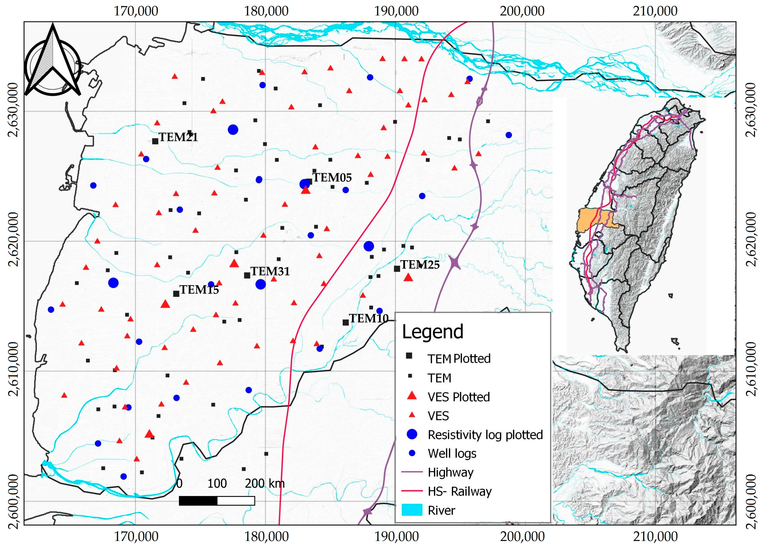
Abstract
:1. Introduction
2. Principle of Time Domain Electromagnetic Method (TEM)
3. Description of the Study Area
4. Geological and Hydrogeological Settings
5. Methods
5.1. Instrumentations
5.2. Data Acquisition, Processing, and Inversion
6. Results
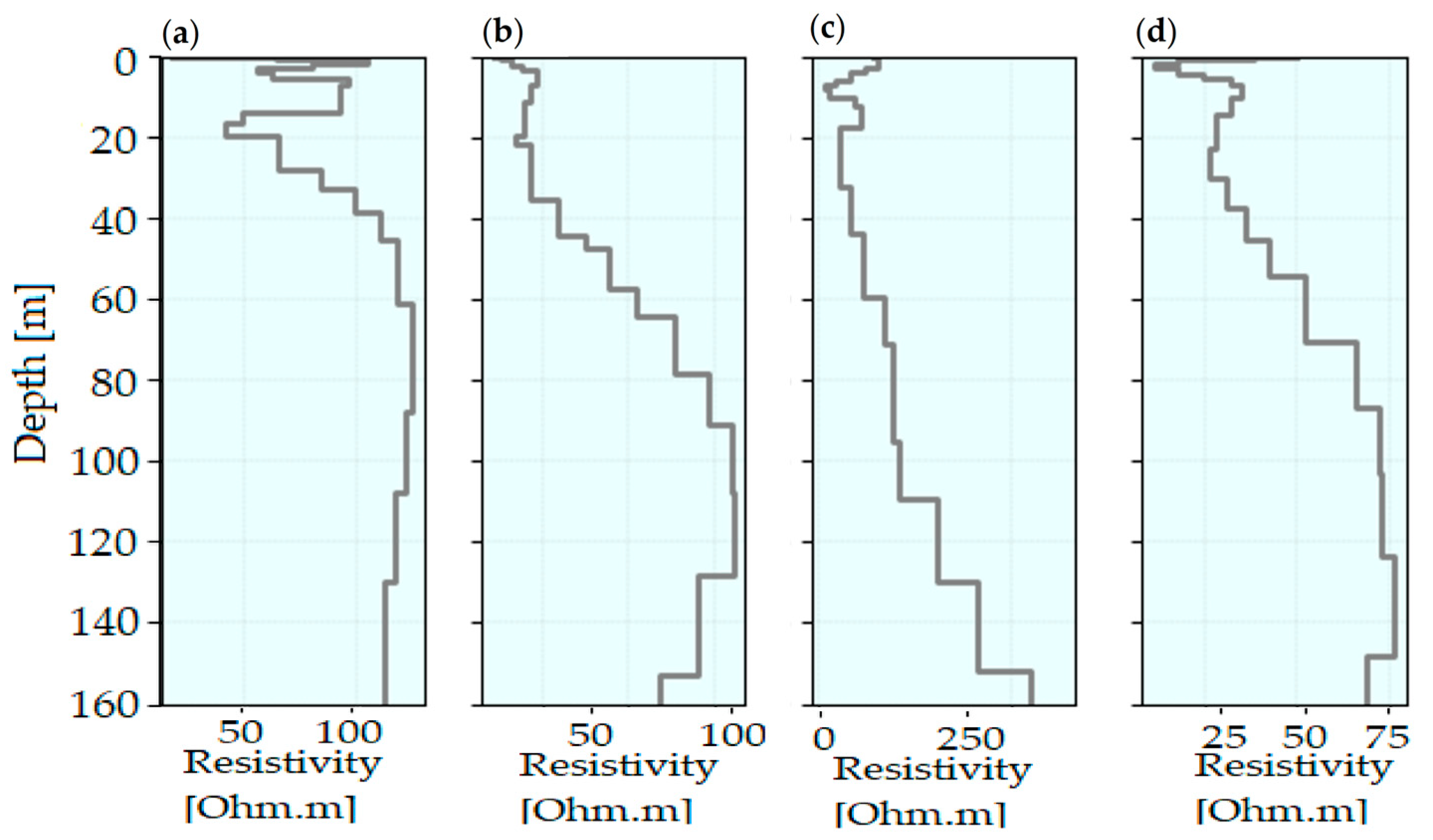
6.1. TEM 1D Models
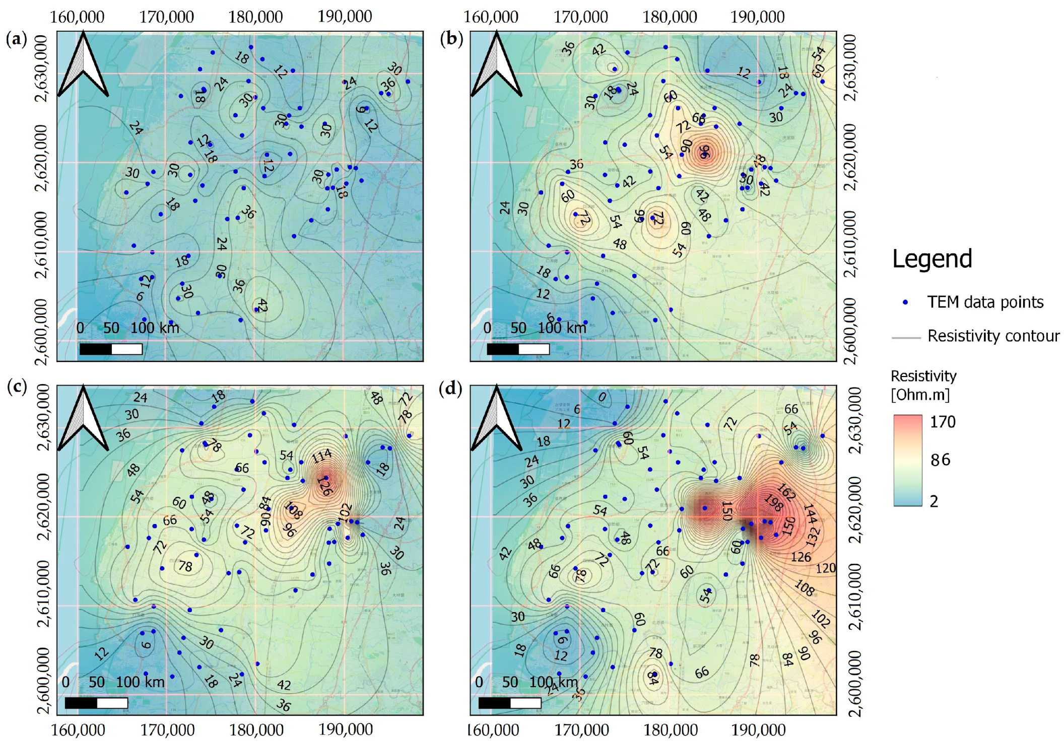
6.2. Slice Maps
7. Discussions
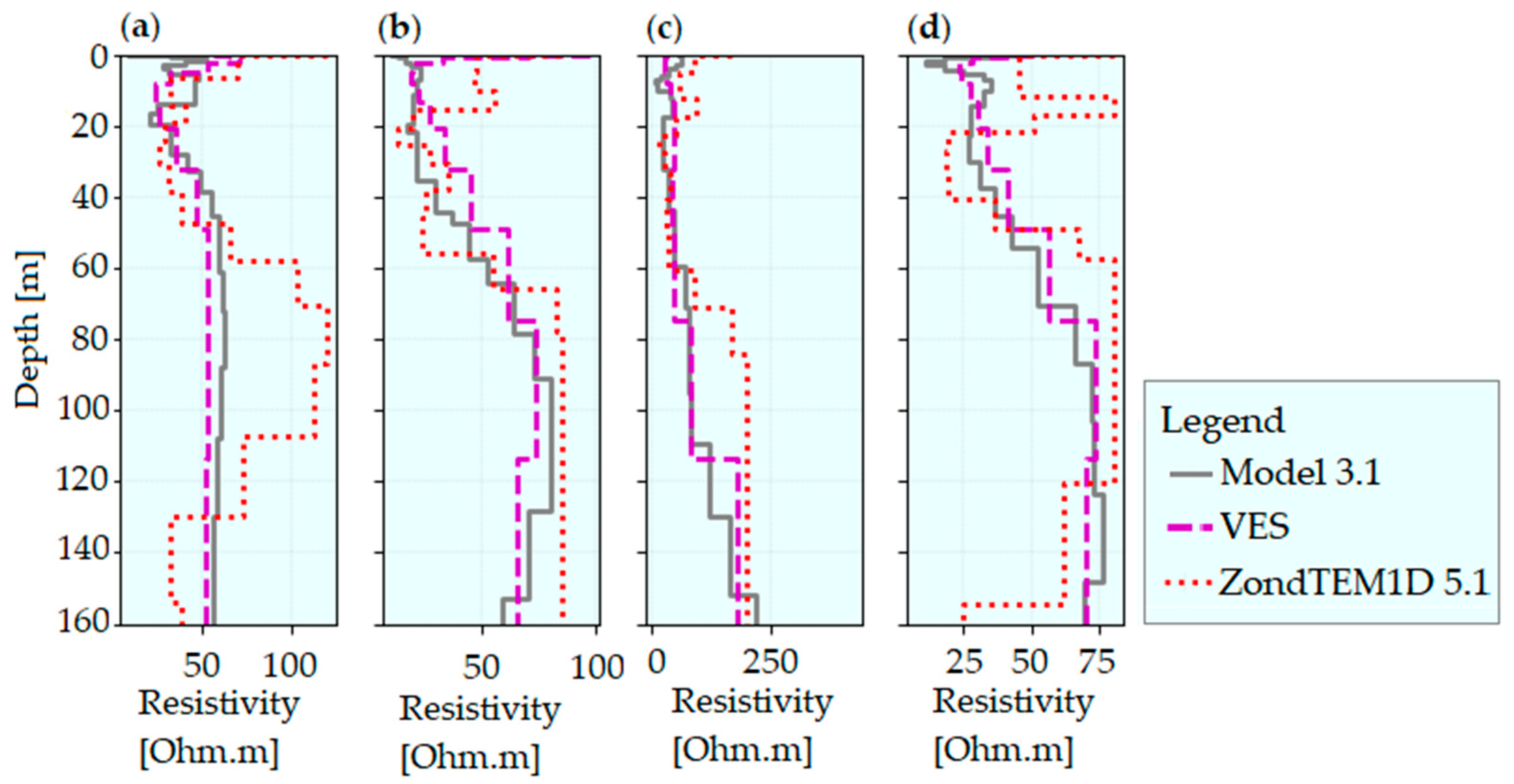
7.1. VES Data as an Initial Model
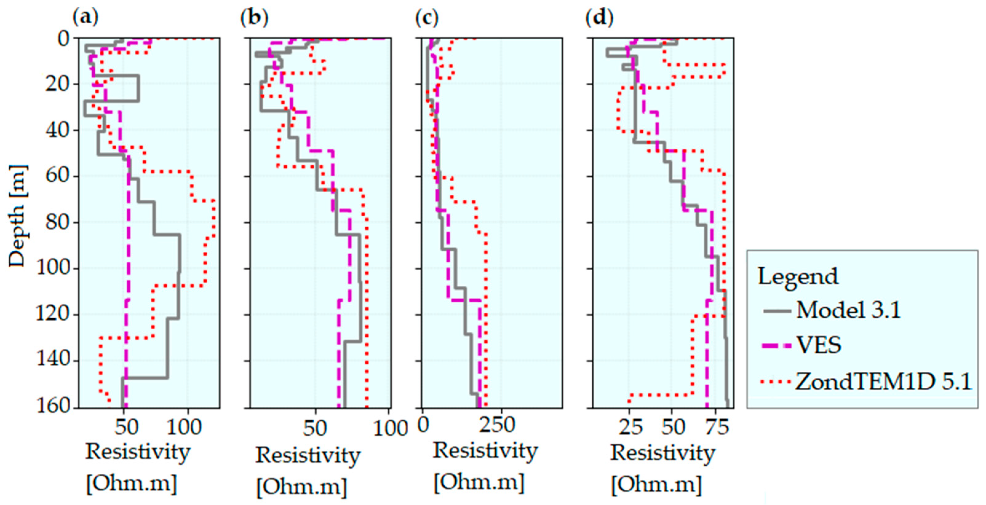
7.2. ZondTEM1D Data as an Initial Model
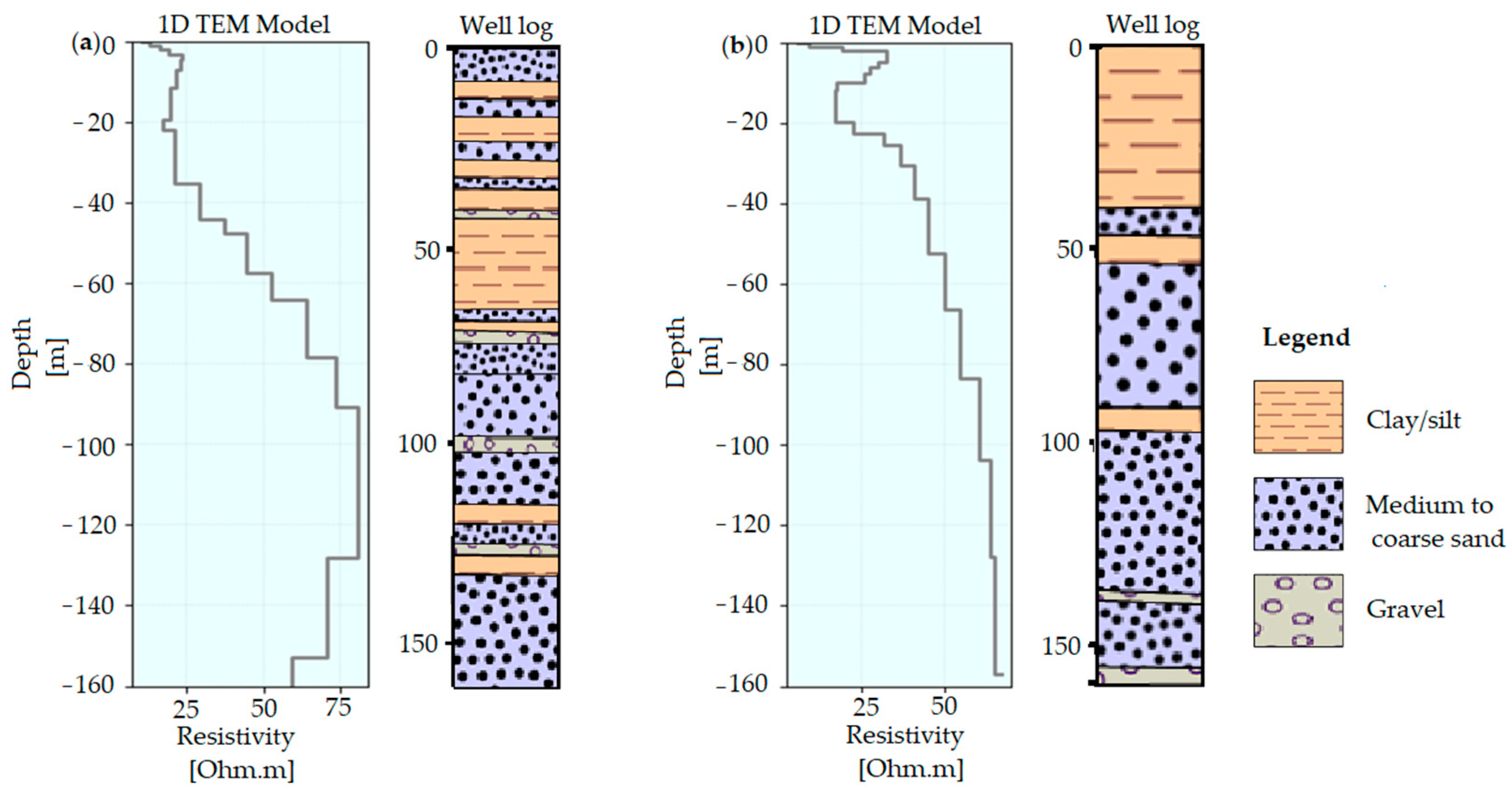
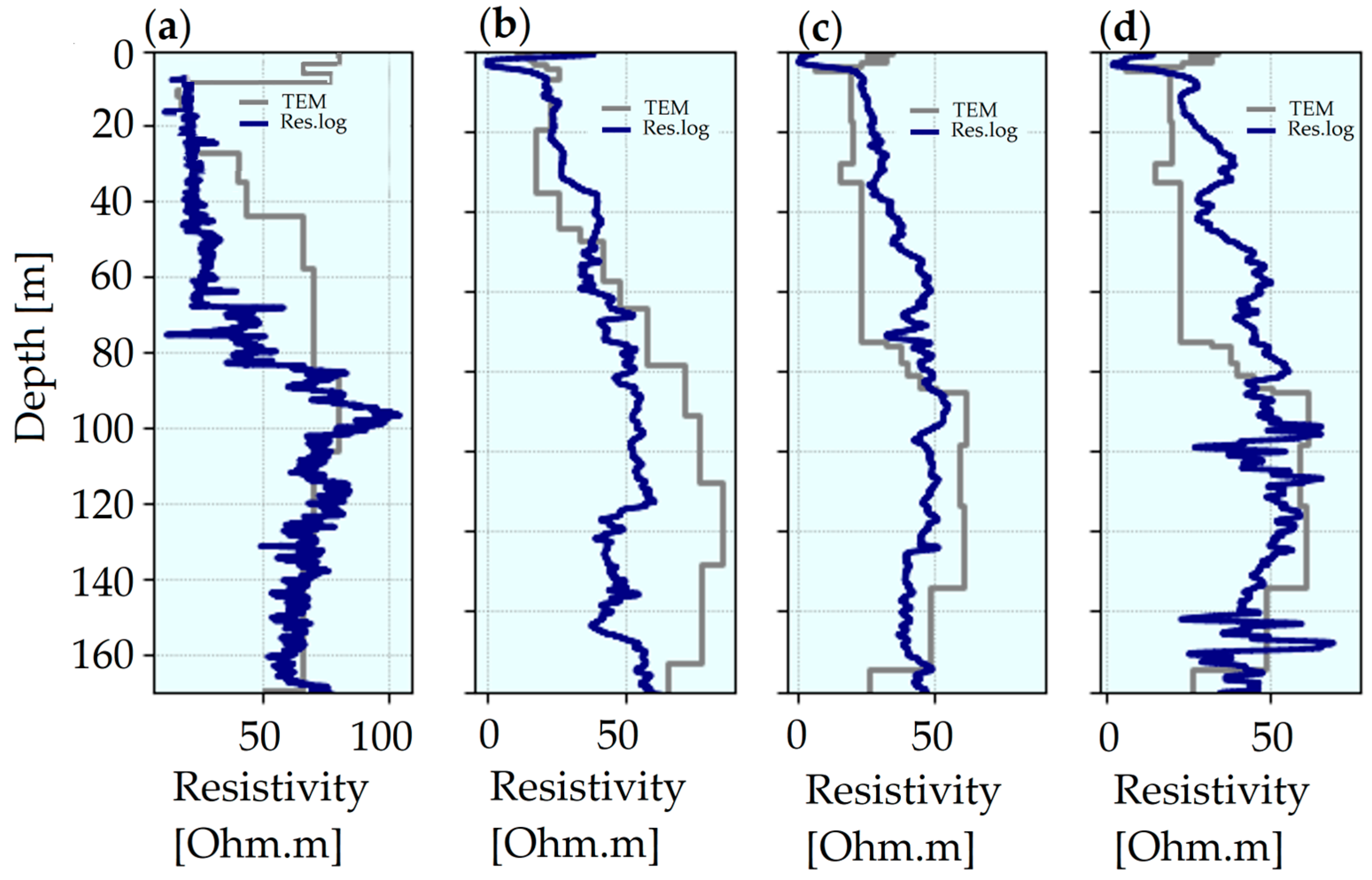
7.3. Comparison of 1D TEM Models and Resistivity Log
8. Conclusions
Author Contributions
Funding
Data Availability Statement
Conflicts of Interest
References
- Kang, S.; Knight, R.; Goebel, M. Improved Imaging of the Large-Scale Structure of a Groundwater System with Airborne Electromagnetic Data. Water Resour. Res. 2022, 58, e2021WR031439. [Google Scholar] [CrossRef]
- Pepin, K.; Knight, R.; Goebel-Szenher, M.; Kang, S. Managed aquifer recharge site assessment with electromagnetic imaging: Identification of recharge flow paths. Vadose Zone J. 2022, 21, e20192. [Google Scholar] [CrossRef]
- Knight, R.; Smith, R.; Asch, T.; Abraham, J.; Cannia, J.; Viezzoli, A.; Fogg, G. Mapping Aquifer Systems with Airborne Electromagnetics in the Central Valley of California. Groundwater 2018, 56, 893–908. [Google Scholar] [CrossRef] [PubMed]
- Hering, J.G.; Ingold, K.M. Water resources management: What should be integrated? Science 2012, 336, 1234–1235. [Google Scholar] [CrossRef] [PubMed]
- Loucks, D.P. Sustainable Water Resources Management. Water Int. 2000, 25, 3–10. [Google Scholar] [CrossRef]
- Zech, A.; Zehner, B.; Kolditz, O.; Attinger, S. Impact of heterogeneous permeability distribution on the groundwater flow systems of a small sedimentary basin. J. Hydrol. 2016, 532, 90–101. [Google Scholar] [CrossRef]
- Dou, X. A critical review of groundwater utilization and management in China’s inland water shortage areas. Water Policy 2016, 18, 1367–1383. [Google Scholar] [CrossRef]
- El-Kaliouby, H.; Abdalla, O. Application of time-domain electromagnetic method in mapping saltwater intrusion of a coastal alluvial aquifer, North Oman. J. Appl. Geophys. 2015, 115, 59–64. [Google Scholar] [CrossRef]
- Erban, L.E.; Gorelick, S.M.; Zebker, H.A. Groundwater extraction, land subsidence, and sea-level rise in the Mekong Delta, Vietnam. Environ. Res. Lett. 2014, 9, 084010. [Google Scholar] [CrossRef]
- Lin, C.-W.; Hwung, H.-H.; Hsiao, S.-C.; Yeh, C.-L.; Hsu, J.-T. Land Subsidence Caused by Groundwater Exploitation in Yunlin, Taiwan. In Proceedings of the ICHE 2016 Proceedings of the 12th International Conference on Hydroscience & Engineering, Tainan, Taiwan, 6–10 November 2016. [Google Scholar]
- Liu, C.-H.; Pan, Y.-W.; Liao, J.-J.; Huang, C.-T.; Ouyang, S. Characterization of land subsidence in the Choshui River alluvial fan, Taiwan. Environ. Geol. 2004, 45, 1154–1166. [Google Scholar] [CrossRef]
- Chen, C.-S. TEM Investigations of Aquifers in the Southwest Coast of Taiwan. Groundwater 1999, 37, 890–896. [Google Scholar] [CrossRef]
- CGS. The Investigation of Hydrogeology in the Choushui River Alluvial Fan, Taiwan; Central Geological Survey of Taiwan: Taipei, Taiwan, 1999. [Google Scholar]
- Christensen, N.B.; Sørensen, K.I. Integrated Use of Electromagnetic Methods for Hydrogeological Investigations. In Proceedings of the 7th EEGS Symposium on the Application of Geophysics to Engineering and Environmental Problems, Boston, MA, USA, 27 March–31 March 1994; European Association of Geoscientists & Engineers: Houten, The Netherlands, 1994. [Google Scholar] [CrossRef]
- Amato, F.; Pace, F.; Vergnano, A.; Comina, C. TDEM prospections for inland groundwater exploration in semiarid climate, Island of Fogo, Cape Verde. J. Appl. Geophys. 2021, 184, 104242. [Google Scholar] [CrossRef]
- Leite, D.N.; Bortolozo, C.A.; Porsani, J.L.; Couto, M.A., Jr.; Campaña, J.D.R.; dos Santos, F.A.M.; Rangel, R.C.; Hamada, L.R.; Sifontes, R.V.; de Oliveira, G.S.; et al. Geoelectrical characterization with 1D VES/TDEM joint inversion in Urupês-SP region, Paraná Basin: Applications to hydrogeology. J. Appl. Geophys. 2018, 151, 205–220. [Google Scholar] [CrossRef]
- Martínez-Moreno, F.; Monteiro-Santos, F.; Madeira, J.; Bernardo, I.; Soares, A.; Esteves, M.; Adão, F. Water prospection in volcanic islands by Time Domain Electromagnetic (TDEM) surveying: The case study of the islands of Fogo and Santo Antão in Cape Verde. J. Appl. Geophys. 2016, 134, 226–234. [Google Scholar] [CrossRef]
- Porsani, J.L.; Bortolozo, C.A.; Almeida, E.R.; Sobrinho, E.N.S.; dos Santos, T.G. TDEM survey in urban environmental for hydrogeological study at USP campus in São Paulo city, Brazil. J. Appl. Geophys. 2012, 76, 102–108. [Google Scholar] [CrossRef]
- Baawain, M.S.; Al-Futaisi, A.M.; Ebrahimi, A.; Omidvarborna, H. Characterizing leachate contamination in a landfill site using Time Domain Electromagnetic (TDEM) imaging. J. Appl. Geophys. 2018, 151, 73–81. [Google Scholar] [CrossRef]
- Abu Rajab, J.; El-Naqa, A. Mapping groundwater salinization using transient electromagnetic and direct current resistivity methods in Azraq Basin, Jordan. Geophysics 2013, 78, B89–B101. [Google Scholar] [CrossRef]
- Vest Christiansen, A.; Foged, N.; Auken, E. A concept for calculating accumulated clay thickness from borehole lithological logs and resistivity models for nitrate vulnerability assessment. J. Appl. Geophys. 2014, 108, 69–77. [Google Scholar] [CrossRef]
- Vignoli, G.; Fiandaca, G.; Vest Christiansen, A.; Kirkegaard, C.; Auken, E. Sharp spatially constrained inversion with applications to transient electromagnetic data. Geophys. Prospect. 2015, 63, 243–255. [Google Scholar] [CrossRef]
- Soupios, P.M.; Kalisperi, D.; Kanta, A.; Kouli, M.; Barsukov, P.; Vallianatos, F. Coastal aquifer assessment based on geological and geophysical survey, northwestern Crete, Greece. Environ. Earth Sci. 2010, 61, 63–77. [Google Scholar] [CrossRef]
- Christensen, N.B.; Christiansen, A.V. Using geophysical survey results in the inference of aquifer vulnerability measures. Near Surf. Geophys. 2021, 19, 505–521. [Google Scholar] [CrossRef]
- Danielsen, J.E.; Auken, E.; Jørgensen, F.; Søndergaard, V.; Sørensen, K.I. The application of the transient electromagnetic method in hydrogeophysical surveys. J. Appl. Geophys. 2003, 53, 181–198. [Google Scholar] [CrossRef]
- Sharlov, M.; Kozhevnikov, N.; Sharlov, R. Lake Baikal—A Unique Site for Testing and Calibration of Near-surface TEM Systems. In Proceedings of the 23rd European Meeting of Environmental and Engineering Geophysics, Malmö, Sweden, 3–7 September 2017. [Google Scholar] [CrossRef]
- Jupp, D.L.B.; Vozoff, K. Stable Iterative Methods for the Inversion of Geophysical Data. Geophys. J. Int. 1975, 42, 957–976. [Google Scholar] [CrossRef]
- Jackson, D.D. Interpretation of Inaccurate, Insufficient and Inconsistent Data. Geophys. J. Int. 1972, 28, 97–109. [Google Scholar] [CrossRef]
- Bleistein, N.; Cohen, J.K. Nonuniqueness in the inverse source problem in acoustics and electromagnetics. J. Math. Phys. 1977, 18, 194–201. [Google Scholar] [CrossRef]
- Verma, S.K. Diffusion of an electromagnetic pulse in a heterogeneous earth. In Deep Electromagnetic Exploration. Lecture Notes in Earth Sciences; Springer: Berlin/Heidelberg, Germany, 1998; pp. 527–565. [Google Scholar] [CrossRef]
- Hung, W.-C.; Hwang, C.; Chang, C.-P.; Yen, J.-Y.; Liu, C.-H.; Yang, W.-H. Monitoring severe aquifer-system compaction and land subsidence in Taiwan using multiple sensors: Yunlin, the southern Choushui River Alluvial Fan. Environ. Earth Sci. 2010, 59, 1535–1548. [Google Scholar] [CrossRef]
- Jang, C.-S.; Liu, C.-W.; Chia, Y.; Cheng, L.-H.; Chen, Y.-C. Changes in hydrogeological properties of the River Choushui alluvial fan aquifer due to the 1999 Chi-Chi earthquake, Taiwan. Hydrogeol. J. 2008, 16, 389–397. [Google Scholar] [CrossRef]
- Liu, C.-W.; Jang, C.-S.; Chen, S.-C. Three-dimensional spatial variability of hydraulic conductivity in the Choushui River alluvial fan, Taiwan. Environ. Geol. 2002, 43, 48–56. [Google Scholar] [CrossRef]
- Sharlov, M.; Buddo, I.; Pisarnitskiy, A.; Misurkeeva, N.; Shelohov, I. Shallow transient electromagnetic method application for groundwater exploration: Case study from Greece. ASEG Ext. Abstr. 2019, 2019, 1–5. [Google Scholar] [CrossRef]
- Spies, B.R. Depth of investigation in electromagnetic sounding methods. Geophysics 1989, 54, 872–888. [Google Scholar] [CrossRef]
- Chen, C.-H.; Wang, C.-H.; Hsu, Y.-J.; Yu, S.-B.; Kuo, L.-C. Correlation between groundwater level and altitude variations in land subsidence area of the Choshuichi Alluvial Fan, Taiwan. Eng. Geol. 2010, 115, 122–131. [Google Scholar] [CrossRef]


Disclaimer/Publisher’s Note: The statements, opinions and data contained in all publications are solely those of the individual author(s) and contributor(s) and not of MDPI and/or the editor(s). MDPI and/or the editor(s) disclaim responsibility for any injury to people or property resulting from any ideas, methods, instructions or products referred to in the content. |
© 2023 by the authors. Licensee MDPI, Basel, Switzerland. This article is an open access article distributed under the terms and conditions of the Creative Commons Attribution (CC BY) license (https://creativecommons.org/licenses/by/4.0/).
Share and Cite
Kassie, L.N.; Chang, P.-Y.; Zeng, J.-R.; Huang, H.-H.; Chen, C.-S.; Doyoro, Y.G.; Lin, D.-J.; Puntu, J.M.; Amania, H.H. Mapping Hydrogeological Structures Using Transient Electromagnetic Method: A Case Study of the Choushui River Alluvial Fan in Yunlin, Taiwan. Water 2023, 15, 1703. https://doi.org/10.3390/w15091703
Kassie LN, Chang P-Y, Zeng J-R, Huang H-H, Chen C-S, Doyoro YG, Lin D-J, Puntu JM, Amania HH. Mapping Hydrogeological Structures Using Transient Electromagnetic Method: A Case Study of the Choushui River Alluvial Fan in Yunlin, Taiwan. Water. 2023; 15(9):1703. https://doi.org/10.3390/w15091703
Chicago/Turabian StyleKassie, Lingerew Nebere, Ping-Yu Chang, Jun-Ru Zeng, Hsin-Hua Huang, Chow-Son Chen, Yonatan Garkebo Doyoro, Ding-Jiun Lin, Jordi Mahardika Puntu, and Haiyina Hasbia Amania. 2023. "Mapping Hydrogeological Structures Using Transient Electromagnetic Method: A Case Study of the Choushui River Alluvial Fan in Yunlin, Taiwan" Water 15, no. 9: 1703. https://doi.org/10.3390/w15091703