A WRF/WRF-Hydro Coupled Forecasting System with Real-Time Precipitation–Runoff Updating Based on 3Dvar Data Assimilation and Deep Learning

Abstract

This study established a WRF/WRF-Hydro coupled forecasting system for precipitation–runoff forecasting in the Daqing River basin in northern China. To fully enhance the forecasting skill of the coupled system, real-time updating was performed for both the WRF precipitation forecast and WRF-Hydro forecasted runoff. Three-dimensional variational (3Dvar) multi-source data assimilation was implemented using the WRF model by incorporating hourly weather radar reflectivity and conventional meteorological observations to improve the accuracy of the forecasted precipitation. A deep learning approach, i.e., long short-term memory (LSTM) networks, was adopted to improve the accuracy of the WRF-Hydro forecasted flow. The results showed that hourly data assimilation had a positive impact on the range and trends of the WRF precipitation forecasts. The quality of the WRF precipitation outputs had a significant impact on the performance of WRF-Hydro in forecasting the flow at the catchment outlet. With the runoff driven by precipitation forecasts being updated by 3Dvar data assimilation, the error of flood peak flow was decreased by 3.02–57.42%, the error of flood volume was decreased by 6.34–39.30%, and the Nash efficiency coefficient was increased by 0.15–0.52. The implementation of LSTM can effectively reduce the forecasting errors of the coupled system, particularly those of the time-to-peak and peak flow volumes.

1. Introduction

Many researchers highlight the coupling of a mesoscale numerical weather prediction model (e.g., the WRF model) with hydrological models as a useful tool for flood prediction [1,2]. This is especially crucial for early warning purposes in unprotected watersheds [3]. Because of the instability of the atmosphere itself, numerical atmospheric models, which are the current main means of precipitation forecasting, cannot accurately forecast the specific occurrence time, location, and intensity of heavy precipitation processes. This poses challenges to the forecasting and early warning of rainstorm-induced flood disasters. Kryza et al. [4] used the WRF model to forecast short-term heavy precipitation in southwestern Poland. The results showed that none of the model configurations could accurately reproduce local heavy precipitation. Hamill et al. [5] applied an ensemble forecasting system to improve the WRF precipitation forecasting ability. Generally, although ensemble forecasting can reflect the forecasting ability or reliability of the real atmosphere to a certain extent, it cannot improve the physical mechanisms of models. Using data assimilation technology to effectively correct errors in the global initial field and lateral boundary conditions of models is key to fundamentally improving their numerical precipitation forecasting capabilities.

Real-time assimilation of high-resolution meteorological observation data can effectively promote the initialization of a numerical atmospheric model for the precipitation process, particularly during severe convective weather, and is an important way of improving the model’s precipitation forecasting ability. The most commonly used data assimilation methods are the optimal interpolation method, three-dimensional variational method (3Dvar) [6,7], four-dimensional variational method (4DVAR) [8,9], and the Kalman filtering method [10]. Among these, 3Dvar has strong stability and high computing efficiency; therefore, the frequency used is the highest [11]. A variational data analysis system called the variational Doppler radar analysis system (VDRAS) was first developed by Sun et al. [12]. Subsequently, Sun and Crook [13] used it for the initialization of short-term forecasts during convective precipitation, and the three-dimensional variational method technology began to be widely used. Lan et al. [14] concluded that 3Dvar impacts the forecast quality by generating initial conditions that represent the state of the atmosphere more accurately. They also showed that 3Dvar is unsuitable for short-term forecasting. Under the right conditions, 3Dvar can increase the model performance after a 24 h runtime, especially after 72 forecast hours. Neyestani et al. [15] applied 3Dvar to convective-scale forecasts, which they investigated using WRF. They verified the 24 h convective-scale precipitation forecasts from the WRF model with and without 3Dvar, and found that the WRF-3Dvar model could forecast precipitation with superior accuracy over the simulation domain, even for the downscaling run. These studies showed that 3Dvar plays an active role in precipitation forecasting.

In recent years, with the development of remote sensing technologies, weather radar has emerged as a new tool for observing disastrous weather owing to its ability to rapidly detect the evolution of cloud and rain structures and obtain high-resolution instantaneous precipitation information [16]. An efficient multi-source data assimilation method dominated by weather radar provides opportunities for further improving precipitation forecasts. Weather radars can measure precipitation millions of times with a spatial resolution of several kilometers and a temporal resolution of several minutes [11]. Compared to existing mesoscale observation platforms, this remarkable advantage due to the high temporal and spatial resolutions has great potential for improving small-scale and short-term precipitation forecasting. At present, many researchers have combined high-resolution observational data with numerical models, which has played a positive role in promoting the development of convective precipitation forecasting, improving the initial states of numerical models, and mitigating instabilities caused by interpolation [17,18,19]. Sugimoto et al. [11] pointed out that assimilating the radial velocity and reflectivity in a 3Dvar system can improve the forecasting ability of the WRF model and applied it to short-term precipitation forecasting. Lagasio et al. [20] evaluated the forecasting ability of the WRF model after assimilating radar reflectivity data and conventional weather station data, and confirmed the importance of rapid updating and intensive data assimilation for improving quantitative precipitation forecasts as well as flash flood forecasts. To study the influence of radar detection radial velocity and reflectivity data assimilation on precipitation forecasting, Souza et al. [21] used the WRF model and its three-dimensional variational assimilation system to test cyclic and acyclic assimilation processes under different initial conditions. The results showed that radar data assimilation plays a fundamental role in improving the performance of convective system simulations and has a positive impact on the short-term forecasting of convective system-related precipitation. Cáceres et al. [22] adopted the WRF and 3Dvar data assimilation to explore a suitable forecasting approach in northeastern Spain. The WRF model combined with the 3DVAR data assimilation method was selected by Zhu [23] to assimilate radar reflectivity and radial velocity data were selected to simulate rainfall, and it was validated with the Integrated Multi-satellitE Retrievals for GPM precipitation data. The results showed that the hourly radar data assimilation can improve the simulated precipitation, and the combination of GPM precipitation data and 3Dvar is a reliable way to forecast stormwater. As a method to improve the accuracy of model prediction, data fusion and assimilation are attracting more and more attention, which makes it possible to forecast floods in areas with complex topography and rainfall.

Limited by the model structure, initial state and input data errors, and parameter identification ability, existing runoff forecasting models involve uncertainties in real-time applications as well as simulation and forecasting accuracy deviations. Model correction can avoid the problem of amending the physical mechanism of the land surface hydrological model. This happens by researching the source of error and correcting the forecasting error according to deviations from the observations. With the development of computer technology, artificial intelligence has been rapidly developing and is widely used in various fields, including hydrology. Artificial neural networks are one of the core artificial intelligence technologies that make the real-time flood forecasting correction technology more comprehensive. Among the many neural networks, recurrent neural networks (RNN) transmit information through an unlimited number of updates, while remembering the state characteristics of time-series data and having good performance in processing and forecasting time-series data [24,25]. Based on an RNN, Hochreiter et al. [24] proposed a long short-term memory (LSTM) neural network with memory units that makes memory information on time series controllable and the LSTM more mature while simulating and forecasting processes in time series. Kratzert et al. [26] trained an LSTM model based on experiments on a large number of basins and found that the LSTM can forecast runoff from meteorological observations, while the pre-trained memory can be transferred to different basins and forecast runoff in cases with no measurements or with only few measured values. Zhang et al. [27] explored the ability of an LSTM model to forecast sewage flow and found significant advantages. In many studies on the application of LSTM to hydrology, LSTM is mostly used for directly forecasting runoff and other characteristic quantities, and there is lack of research on improving the runoff forecasting ability by combining it with physical hydrological models.

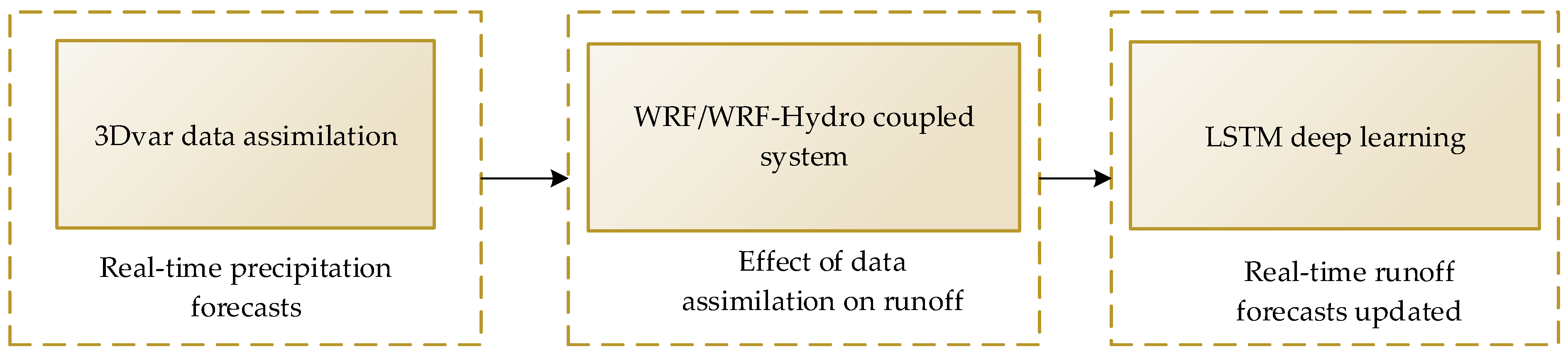
Previous research has focused on using radar precipitation measurements or mesoscale numerical weather prediction models for precipitation forecasting, and then driving hydrological models for runoff forecasting. Traditional real-time correction techniques focus only on runoff forecasting without considering real-time updating and correcting the forecasted precipitation. In many studies on the application of LSTM in the hydrological field, LSTM is mostly used to directly predict the characteristic variables of the runoff, lacking research on improving the runoff forecasting ability by combining with the hydrological models. In this study, a WRF/WRF-Hydro coupled system was established for precipitation and runoff forecasting in mountainous catchments of northern China. A three-dimensional variational data assimilation method was adopted based on the weather radar, supplemented with traditional meteorological monitoring data, to perform multi-source data assimilation and improve the precipitation forecasting ability of the WRF model. Based on the construction of error time series, LSTM was used to correct the forecasted runoff from the WRF/WRF-Hydro coupled system, thereby further improving the accuracy of the forecasted runoff. Through the dual factor correction of precipitation and runoff, the forecasting ability of the coupling forecasting system can be effectively improved. The flow chart of this study is shown in Figure 1.

2. Study Area and Storm Events

The Daqinghe Basin, situated in the middle and upper regions of the Haihe Basin in northern China, comprises tributaries that mainly originate from the Taihang Mountains or surrounding foothills and are subject to a warm temperate continental monsoon climate. The basin spans an area of 43,060 km² and is susceptible to frequent flooding, primarily caused by heavy precipitation during the flood season, which generates floods in upstream mountainous areas and leads to disasters in downstream areas. However, human activity, climate change, and inadequate protection measures have resulted in reduced vegetation coverage, irregular forest vegetation structures, and diminished water conservation in the upper reaches of the Daqinghe Basin. Owing to the seasonal characteristics of the Daqing River, very little runoff is supplied by precipitation in the basin during the dry season, and only when there is sufficient precipitation can runoff flow into the channel. In addition, local groundwater overexploitation is severe, resulting in little to no baseflow.

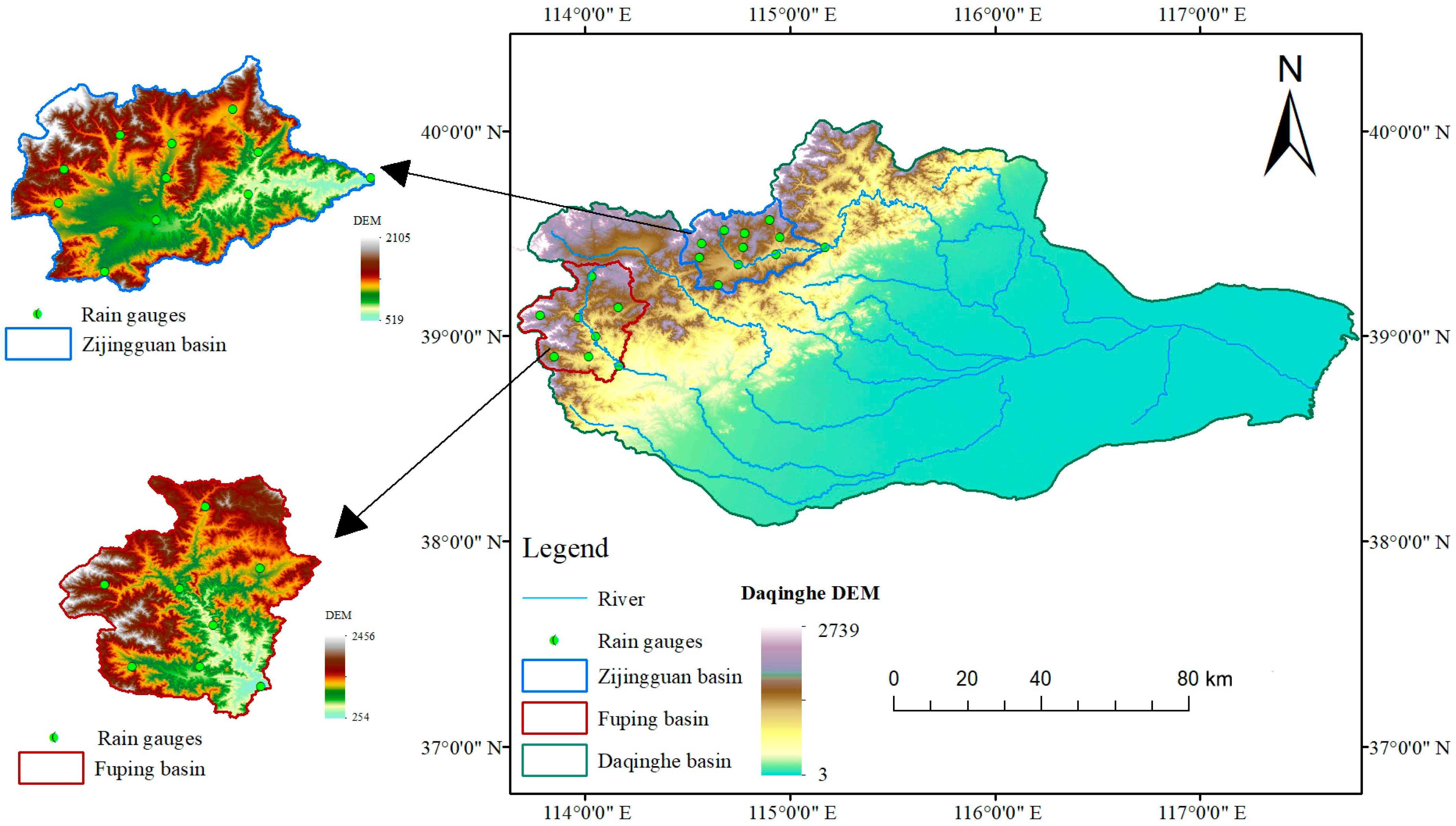
In this study, the Fuping Basin in the southern branch of the Daqing River Basin and the Zijingguan Basin in the northern branch of the Daqing River Basin were used as study areas for conducting an atmosphere–hydrology coupling simulation with real-time updating. The Fuping Basin is located at 113°45′–114°32′ E and 39°22′–38°47′ N, with a watershed area of 2210 km². The entire territory is mountainous and can be divided into deep and shallow mountainous areas according to the terrain. The elevations of deep mountainous areas are higher than 800 m, while those of the shallow mountainous areas are between 200 and 800 m. The Zijinguan Basin is located at 114°28′–115°11′ E and 39°13′–39°40′ N, with a watershed area of 1760 km². The two catchments are located in the Taihang mountain section and the upper reaches of the Daqinghe basin, with the maximum and the minimum elevation being 2286 m and 200 m above sea level. The elevation decreases from northwest to southeast and changes greatly. The steep terrain leads to a short confluence time of the flood, which together with high-intensity, short-duration precipitation is prone to cause severe flood disasters. They are concentrated in areas with thin soil layer and low vegetation coverage especially. Soil vadose zones are often in a state of water shortage. The runoff generation process is accompanied by a mixed mechanism of infiltration capacity excess and storage capacity excess. There were eight precipitation stations in the Fuping Basin and 11 precipitation stations in the Zijinguan Basin. The geographical location, topography, and distribution of the precipitation stations in the study area are shown in Figure 2. The duration and cumulative precipitation of 10 storm events are shown in

Table 1. Duration, accumulated precipitation, and maximum stream flow of 10 selected 24 h storm events.

Event ID	Catchment	Precipitation Duration	Accumulated Precipitation (mm)	Maximum Flow (m3/s)
1	Fuping	29 July 2007 20:00–30 July 2007 20:00	63.38	29.7
2	Fuping	30 July 2012 10:00–31 July 2012 10:00	50.48	70.7
3	Fuping	1 September 2012 06:00–2 September 2012 06:00	40.30	13.7
4	Fuping	11 August 2013 07:00–12 August 2013 07:00	30.82	46.6
5	Fuping	25 July 2016 00:00–26 July 2016 00:00	12.84	1740.0
6	Zijingguan	22 May 2007 00:00–22 May 2007 24:00	39.52	4.1
7	Zijingguan	10 August 2008 00:00–10 August 2008 24:00	45.53	6.8
8	Zijingguan	21 July 2012 04:00–22 July 2012 04:00	172.17	2580.0
9	Zijingguan	6 June 2013 22:00–7 June 2013 22:00	52.06	9.8
10	Zijingguan	19 July 2016 00:00–20 July 2016 00:00	59.43	53.4

. Duration, accumulated precipitation, and maximum stream flow of 10 selected 24 h storm events. The average annual precipitation in the basin is approximately 600 mm, with most of the precipitation occurs from late May to early September.

The 24 h precipitation accumulation was computed using the Thiessen polygon method, which averages the observations from rain gauges. Due to various limitations, there is no optimal spatial interpolation method for spatial data interpolation. For different spatial variables, the so-called optimal interpolation method is relative in different regions and spatiotemporal scales. Therefore, the article adopts the Thiessen polygon method used by researchers in the same watershed [28,29].

In this study, the evenness of storm events was quantitatively evaluated in the spatial and temporal dimensions using the variation coefficient Cv.

$$Cv=\sqrt{\frac{1}{N}\sum _{j=1}^N\left(\frac{X_j}{\overline{X}}-1\right)}.$$

(1)

In the spatial dimension, $X_j$ is the accumulated 24 h precipitation at rain gauge j, $\overline{X}$ is the average of $X_j$, and N is the number of rain gauges. In the temporal dimension, $X_j$ is the average hourly precipitation from all rain gauges at time j and N is the number of hours. A higher Cv value corresponds to more uneven precipitation distribution.

Table 2. Precipitation evenness of the selected 24 h storm events in space and time.

Event ID	1	2	3	4	5	6	7	8	9	10
Spatial Cv	0.398	0.193	0.141	0.740	0.365	0.149	0.459	0.610	0.426	0.273
Temporal Cv	0.601	1.082	0.882	2.393	1.477	0.925	1.378	1.887	1.887	2.745

shows the Cv values of the four storm events in both spatial and temporal dimensions.

3. Data and Experimental Design

3.1. WRF Model Settings

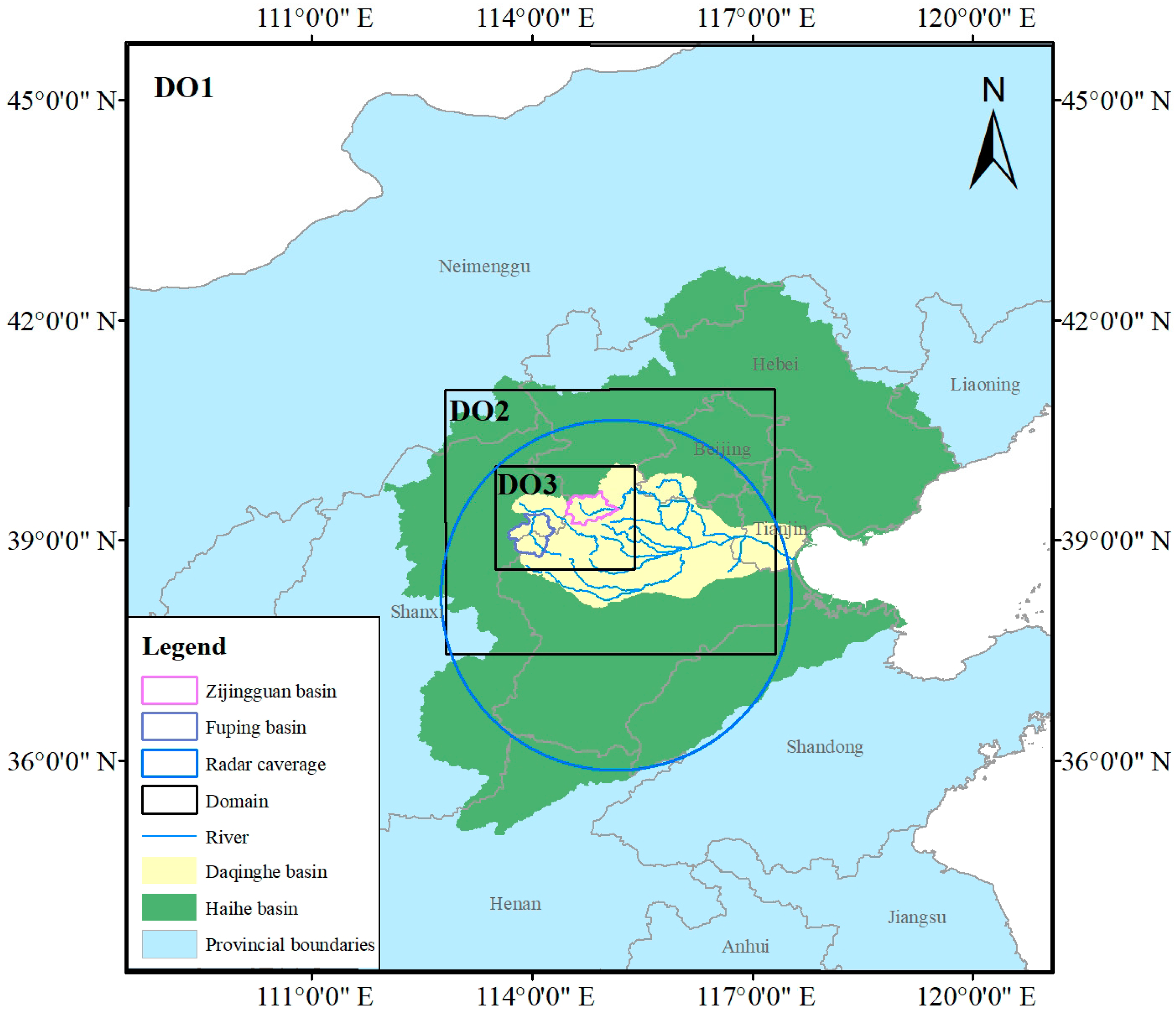
To ensure that the spatial resolution of the nested grid set was as close as possible to that of the radar data, a three-layer nested grid was used. Setting the outermost grid range was conducive for assimilating large-scale GTS data, making the model operation more stable. The innermost grid covered the entire study area. The nesting ratio of the adjacent nesting layers was set to 1:3, and the grid sizes were 1, 3, and 9 km. The inner and outer grids provide two-way feedback in the WRF model. The grid center of the study area was 39°26′00″ N, 114°46′00″ E, and the innermost nested grid (Domain 3) was 145 × 115 km². The second-level nested grid (Domain 2) was 450 × 360 km², covering the radar scanning range, and the outermost nested grid (Domain 1) was 1260 × 1260 km². The nested grid and radar observation ranges in the study area are shown in Figure 3 and

Table 3. WRF model nested grid settings.

Nesting Grid	Horizontal Resolution (km)	Nested Grid Area (km)	Number of Grids	Downscaling Ratio
Domain 1	9	1260 × 1260	140 × 140	/
Domain 2	3	450 × 360	150 × 120	1:3
Domain 3	1	145 × 115	145 × 115	1:3

. The WRF model nested grid settings are shown. The three nested areas in this study were vertically divided into 40 layers. The top air pressure was 50 hPa [30], and the WRF model integration time step was 6 s. The WRF model was set to output simulation results every 1 h. The precipitation output of the WRF model was used to drive the WRF-Hydro model. Because the study basins are located in the mid-latitude region, the Lambert projection was selected. The initial and lateral boundary conditions for forecasting were provided by the 1 × 1° Global Forecasting System (GFS). The GFS data are real-time data provided by the National Environmental Forecasting Center (NCEP) and are updated every 6 h. Because the GFS data are released in real time, they are often used as the initial driving force for precipitation forecasting in the WRF model [31].

The simulation and forecasting capabilities of the model are highly dependent on the parameterization scheme. The scheme selected in this study may be applicable to precipitation processes in one region, but not to those in other regions [32]. Because it is difficult to determine the most suitable scheme for future precipitation, the parameterization scheme is usually determined in advance for practical applications [33]. In this study, the selection of the physical parameterization scheme was based on the sensitivity test results of the parameterization scheme for the same basin as that in Tian et al. [34,35]. The parameterization details that had a significant impact on the precipitation used in the assimilation test are listed in

Table 4. Details of the parameterizations used in the assimilation experiments.

Number	Parameterization	Chosen Option
1	Microphysics scheme	WSM6
2	Longwave radiation	Rapid Radiative Transfer Model (RRTM)
3	Shortwave radiation	Dudhia
4	Land surface scheme	Noah
5	Planetary boundary layer	Mellor–Yamada–Janjic (MYJ)
6	Cumulus convection	Kain–Fritsch (KF)

. Details of the parameterizations used in the assimilation experiments are shown. Among them, the cumulus convection schemes for the 3 and 1 km grids were closed.

3.2. The 3Dvar Data Assimilation of WRF

Data assimilation combines observational data with the background forecasting of the mesoscale atmospheric model and their respective error statistics to improve the initial state of the atmosphere. Variational data assimilation is realized by the iterative minimization of specified functions. The initial state of the model is constantly adjusted by iteration, and the difference between forecasting and observation is reduced according to the following calculation correction:

$$J(x)=J_b(x)+J_o(x)$$

(2)

$$J_b\left(x\right)=\frac{1}{2}{\left(X-X_b\right)}^T{B}^{-1}\left(X-X_b\right)$$

(3)

$$J_o(x)=\frac{1}{2}{\left(H(X)-Y_0\right)}^T{R}^{-1}\left(H(X)-Y_0\right)$$

(4)

The variational problem can be summarized by solving an analytical variable to make a target functional that measures the distance between the analytical variable and the background. The observation reaches the minimum; this occurs by finding the initial state X of the model that minimizes J(x) (Equation (2)), which comprises the background component J_b(x) (Equation (3)) and observation component J_o(x) (Equation (4)) [36], where X_b is the background field, B is the background error covariance matrix, Y₀ is the observation vector, H is the observation operator projecting the model variable from the model space to the observation space through y = H(x) for comparison with the observation results, R is the observation error covariance matrix, R = E + F, E is the instrument observation error covariance matrix, and F is the observation representative error covariance matrix.

The three-dimensional variational data assimilation method takes into account all observed data simultaneously, while ignoring changes over time during the assimilation process; hence, its operation is more efficient than that of the four-dimensional variational data assimilation. Assimilation algorithms in mesoscale numerical atmospheric models vary based on the observational data. For example, the 3Dvar assimilation system can assimilate 19 types of data, including conventional and unconventional observational data. When using the WRF model for precipitation forecasting, the most significant difference between introducing and not introducing data assimilation was whether the background was corrected and close to the real atmospheric state or not. The assimilation data used in this study were high-resolution observational, radar, and conventional meteorological data. The 3Dvar assimilation system processes the radar reflectivity and GTS data differently, primarily during the data preprocessing stage. GTS data assimilation follows a simpler principle than radar data assimilation. The assimilation of GTS data is based on the LITTLE_R format storage, and the ob.ascii file is obtained after running the file using obsproc.exe, and 3Dvar can easily recognize the downloaded GTS data. However, the principles of radar data assimilation are different. Radar reflectivity data are directly output after radar signal processing, and 3Dvar converts the assimilation of the rainwater mixing ratio (q_r) into an assimilation of reflectivity based on the observation operator of the radar reflectivity [13].

$$Z=43.1+17.5\log \left(\rho q_r\right)$$

(5)

where, ρ is the air density and Z is the radar reflectivity. This relation is derived analytically by assuming the Marshall–Palmer distribution of raindrop size. Simultaneously, the pixel-based radar reflectivity is assimilated directly into 3Dvar by stating the latitude and longitude of the pixel center and the height of the radar beam above that pixel.

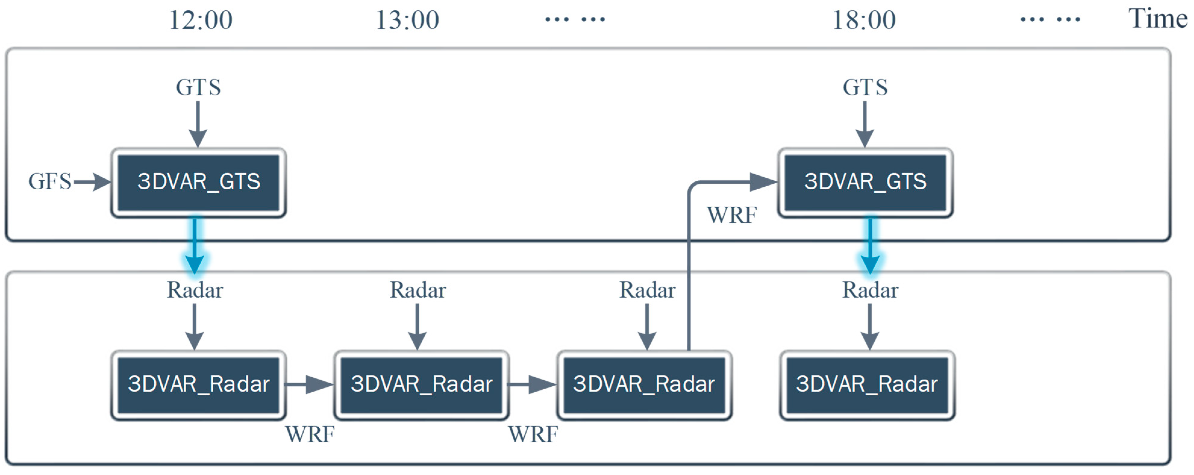
Although weather radar data can provide high-resolution instantaneous precipitation information, their coverage is limited compared to that of the GTS data; thus, they are more suitable for assimilation at small and medium scales. In this study, radar data were only assimilated in Domain 2, as the radar scanning radius used was 250 km, and its coverage area was between the outermost and innermost nested grids, similar to that of Domain 2. GTS data were complementary to the radar data, with wide coverage and low spatial density. Therefore, the GTS data were assimilated into Domain 1. As GTS data were updated every 6 h, in all assimilation schemes, GTS data were assimilated only at 6:00, 12:00, 18:00, and 24:00 after the beginning of precipitation, and radar data were assimilated every hour. Details can be seen in Figure 4. In this study, CV3, which is the error covariance of the global background constructed by the NCEP, was selected because of its wide applicability and adaptability for numerical atmospheric forecasting in any region.

3.3. Observations for 3Dvar Assimilation

3.3.1. Radar Reflectivity

This study utilized radar reflectivity data obtained from an S-band Doppler radar located in Shijiazhuang City. The scanning area radius of the Shijiazhuang S-band radar was 250 km and the effective scanning radius was 230 km, thereby completely covering the Fuping and Zijingguan research areas. The radar completed a volume scan every 6 min, scanning nine levels. The quality of the radar data was controlled before assimilation, supported by the Integrated Meteorological Information Sharing Platform (CIMISS) of the China Meteorological Administration, to remove interference factors, the basic parameters of which are shown in

Table 5. Basic parameters of the Shijiazhuang radar.

Parameters	Information
Location	38.5°, 114.68°
Administrative location	Shijiazhuang
Antenna diameter	1.3 m
Emission frequency	2.7~3.0 GHz
Observation radius	250 km
Effective radius of observation	230 km
Spatial resolution	1 km
Sweep time	6 min
Beam angles	0.5°, 1.5°, 2.4°, 3.4°, 4.3°, 6.0°, 9.9°, 14.6°, 19.5°

. The basic parameters of the Shijiazhuang radar, radar location, and coverage area are shown in Figure 3.

3.3.2. GTS Data

The GTS data utilized in this study were part of a real-time release of global observation data provided by the National Center for Atmospheric Research (NCAR) of the United States, updated every six hours. This collection of near-ground and upper-air meteorological observation data included variables such as air temperature, pressure, wind speed, and humidity [37]. To ensure compatibility with 3Dvar, a shell script was employed to convert the decoded data into a recognizable format, which was then assimilated concurrently with the radar reflectivity data. During the assimilation process, GTS data were directly interpolated into a background pattern and corrected using a specific algorithm.

3.4. WRF-Hydro Model Settings

The WRF/WRF-Hydro coupled system consists of two components, namely the WRF model that forecasts precipitation and the WRF-Hydro model that forecasts runoff. In this study, the input of the WRF-Hydro model was provided by the WRF precipitation forecast, which assimilates radar reflectivity every hour and GTS every six hours

Table 6. Basic settings of the uncoupled WRF-Hydro modeling system.

Subject	Chosen Option
Nest identifier	3
Hydro output interval	1 h
Land surface scheme	Noah
Regrinding (nest) Factor	10
soil column	2 m
Four soil layer thickness	10 cm, 30 cm, 60 cm, 100 cm
Subsurface routing	Yes
Overland flow routing	Yes
Channel routing	Yes with diffusive wave
Baseflow bucket model	No
Main parameter value	REFKDT = 2.5
	MannN = 1.5
	OVROUGHRTFAC = 0.1
	RETDEPRTFAC = 1

. The basic settings of the uncoupled WRF-Hydro modeling system show the basic settings adopted for the WRF-Hydro model, which operated only within the innermost grid (Domain 3; 1 km resolution) of the WRF model, with a sub-grid resolution of 100 m.

During preparation for running the WRF-Hydro model, the key runoff generation and concentration parameters of the model, including the runoff infiltration parameter (REFKDT), channel Manning roughness parameter (MannN), surface retention depth scaling parameter (RETDEPRTFAC), and overland flow roughness scaling parameter (OVROUGHRTFAC), were calibrated using the method of gradual parameter calibration [38,39]. Based on the sensitivity analysis and automatic optimization in the study area, the final parameter values used in the study were REFKDT = 2.5, MannN = 1.5, RETDEPRTFAC = 1, and OVROUGHRTFAC = 0.1. The specific calibration process was described by Liu et al. [40].

3.5. Long Short-Term Memory (LSTM) Network

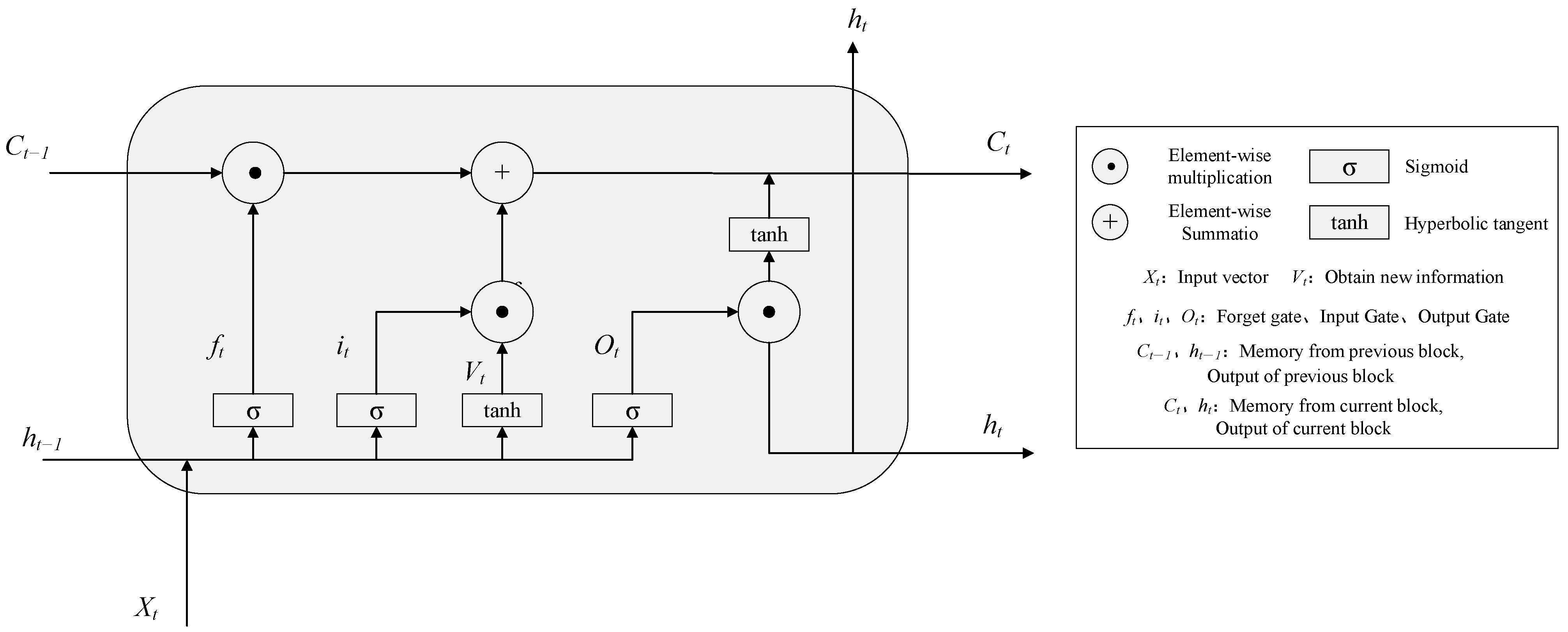
The LSTM network is a special cyclic neural network that allows previous input information to be stored inside it, thereby affecting the output of the network. Compared with traditional cyclic neural networks, LSTM adds memory cell units to the hidden layer, which can better remember longer historical information. A schematic diagram of the LSTM deep-learning model is shown in Figure 5.

In general, the numbers of hidden layers and neurons in each layer can significantly influence the learning and forecasting capabilities of the LSTM model. An excessive number of hidden layers and an excessive number of neurons in each layer can lead to overfitting. Overfitting occurs when the model network memorizes the characteristics of the training data excessively, thereby resulting in an ideal performance during the training stage and large errors during the forecasting stage. The number of hidden layers of the LSTM model selected in this study was one [41,42], while the number of neurons was selected by a trial calculation method. Through trials with different numbers, it was found that the number of neurons, n = 32, minimized the mean square error of the model after multiple training sessions; hence, this number was selected as the number of hidden neurons. This study forecasted the runoff error for the next hour in units of hours by constructing an error sequence. Point-by-point forecasting meant that we only forecasted a single point each time, plotted this point as a forecast, and subsequently took the next data listed along with the full testing data. Finally, the forecasted error series was added to the hydrological forecast results to complete the real-time correction of the coupled hydrological forecast system.

3.6. Evaluation Indicators

The root mean square error (RMSE), mean bias error (MBE), and critical success index (CSI) were used to evaluate the simulated precipitation of the WRF (see Equations (6)–(8)). RMSE and MBE are the most widely used error metrics. RMSE is used to measure the deviation between simulated and observed values. The lower the value of RMSE, the more reliable the prediction, and RMSE should be more useful when major errors are particularly undesirable [43]. MBE represents the average degree of deviation between predicted and actual values, and is a quantitative indicator that can be used to represent the accuracy of the prediction model. After the analysis of the indices, CSI/RMSE was used as the comprehensive evaluation index to explore the more intuitive responses of different precipitation types to forecast errors at the temporal and spatial scales.

$$RMSE=\sqrt{\frac{1}{M}\sum _{i=1}^M{\left(Q_i^{\prime }-Q_i\right)}^2},$$

(6)

$$MBE=\frac{1}{M}\sum _{i=1}^M\left(Q_i^{\prime }-Q_i\right),$$

(7)

$$CSI=\frac{1}{M}\sum _{i=1}^M\frac{H_i}{H_i+S_i+R_i}.$$

(8)

In Equations (6) and (7), for the spatial dimension, Q_i′ and Q_i denote the observed and forecasted accumulated 24 h rainfall, respectively, at each rain gauge i. M is the number of rain gauges, which is 8 for the Fuping catchment and 11 for the Zijingguan catchment. In the temporal dimension, Q_i′ and Q_i are the average areal precipitation of the observation and forecast, respectively, at each time step i. Time M was 24, thereby representing the number of time steps. The specific definitions are listed in

Table 7. Meanings of variables in Equations (6) and (7).

Letter	For the Spatial Dimension	For the Temporal Dimension
Qi′	Observation of 24 h precipitation accumulations at each rain gauge	Average areal precipitation of observation
Qi	Forecasting of 24 h precipitation accumulations at each rain gauge	Average areal precipitation of forecasting
i	Rain gauge ID	Each time step
M	Total numbers of rain gauges	24 h

. The meanings of variables are depicted in Equations (6) and (7).

CSI [44] denotes the percentage of correct simulations between forecast and observations, with 1 indicating a perfect score. The CSI calculation depends on whether it rains. Because the essence of the WRF model simulation is to solve the equations, it is inevitable that the precipitation calculation result will be close to zero. The CSI calculation was based on a rain/no rain contingency table (

Table 8. Rain/no rain contingency table for the WRF simulation against observations.

Forecasting/Observation	Yes (>0.01 mm)	No
Yes	hits (H)	misreports (R)
No	misses (S)	/

).

The classified variables H, R, and S represent whether the forecasted and observed values in a certain observation period or position are greater than 0.01. If both the forecasted and observed values are greater than 0.01, i.e., precipitation is captured in the model, then H + 1; if the forecasted value is greater than 0.01 and the observed value is less than or equal to 0.01, i.e., the model misreports precipitation, then R + 1; if the forecasted value is less than or equal to 0.01 and the observed value is greater than 0.01, i.e., the precipitation is missed in the model, then S + 1. If both the forecasted and observed values are equal to 0.01, the model accurately forecasts a scenario without precipitation.

For the spatial dimension, the forecasted precipitation was compared with observations at rain gauge locations to calculate the indices H, R, and S at time i. Subsequently, the values of the indices at all times were averaged to obtain the CSI according to Equation (8). M is the total number of iterations. In this study, time i was consistent with the output frequency of the model, which was 1 h. That is, CSI is the average value of H/(H + R + S) for each hour of the 24 h precipitation duration. Similarly, for the temporal dimension, the indices in Table 7 were calculated based on time-series data obtained for the simulated and observed areal precipitation at rain gauge i. The values of the indices at all rain gauges were then averaged to produce the final CSI value, based on Equation (8). Here, M refers to the total number of rain gauges rather than the simulation time.

The Nash efficiency coefficient (NSE), relative error of peak flow (R_f), relative error of flood volume (R_v) and absolute error of peak time (T) were used to evaluate the runoff simulated by the WRF-Hydro model (see Equations (6)–(8)). The NSE was used to verify the reliability of the hydrological model simulation results. RMSE was used to measure the deviation between the forecasted and observed values. R_f is the relative error of the flood peak reflecting the credibility of the simulated flood peak, and R_v is the relative error of the flood volume reflecting the credibility of the simulated flood volume. T is the time difference between the actual and forecasted peak times, which was used to represent the error in the peak time forecasting.

$$NSE=1-\frac{\sum _{i=1}^N{(R_i^{\prime }-R_i)}^2}{\sum _{i=1}^N{(R_i-\overline{R})}^2},$$

(9)

$$R_v=\left(R_v^{\prime }-R_v\right)/R_v,$$

(10)

$$R_f=\left(R_f^{\prime }-R_f\right)/R_f,$$

(11)

T = |T₁ − T₂|,

(12)

where R_i′ is the runoff forecast value of the ith hour in the flood process, R_i is the measured runoff value in the ith hour during the flood process, N is the time step, $\overline{R}$ is the average value of R_i, R_f′ is the forecasted value of the peak flow of each flood, R_f is the measured value of the peak flow of each flood, R_v′ is the forecasted value of the flood volume of each flood, and R_v is the measured value of flood volume of each flood. T₁ is the actual peak time; T₂ is the forecast peak time.

4. Results

4.1. Real-Time Precipitation Forecasts Based on 3Dvar Data Assimilation

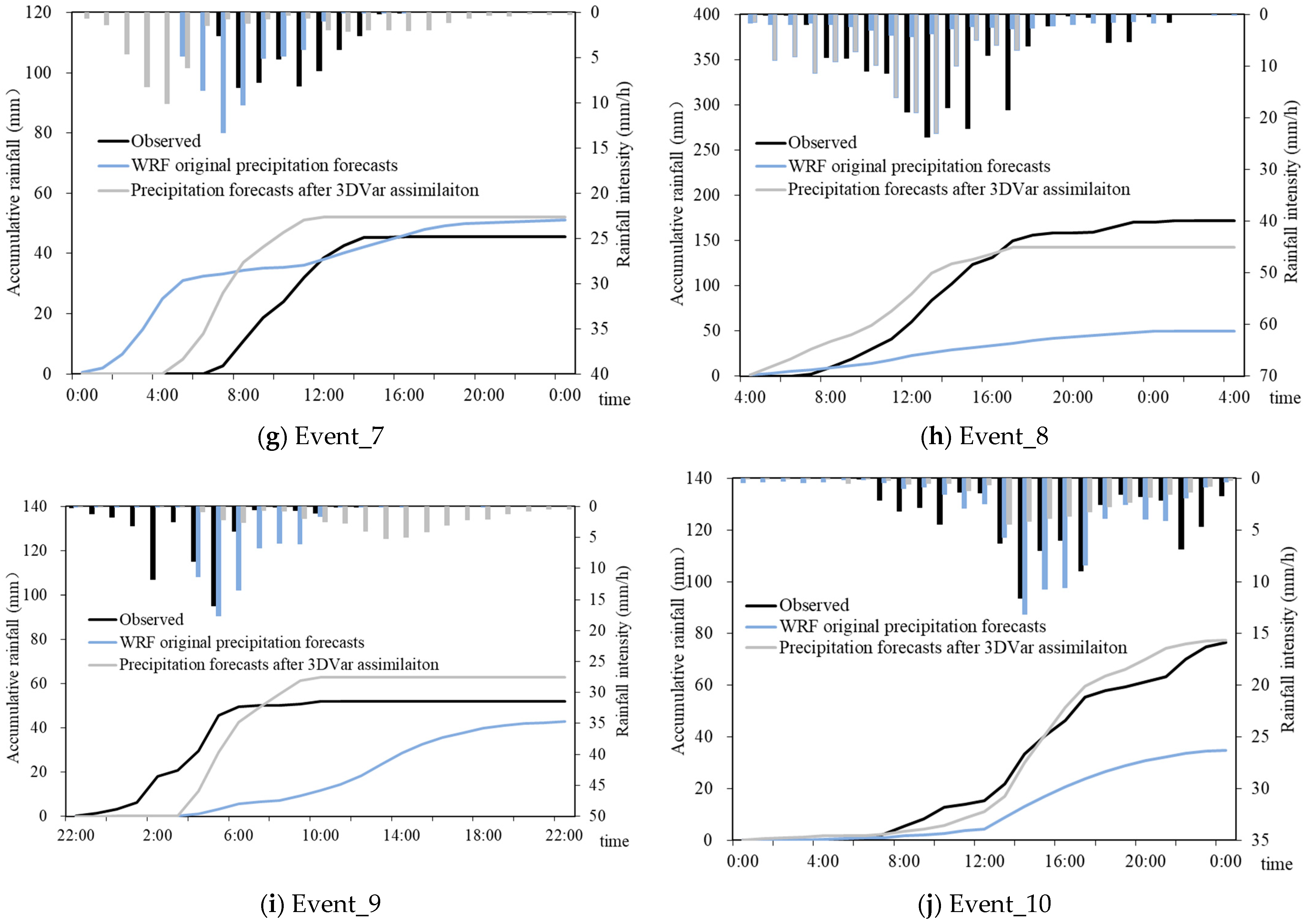
Figure 6 illustrates the real-time precipitation forecasting results of the WRF model after the 3Dvar data assimilation. Cumulative precipitation was computed based on the mean precipitation of each grid point within the study area. When the grid area inside the basin boundary accounted for over 50% of the grid area, the precipitation value of the grid points was included in the calculation of precipitation accumulation. The Thiessen polygon method was used to average the precipitation gauge observations and calculate the observed cumulative precipitation. In Figure 6, the observed accumulative curves are represented by black solid lines, the precipitation forecasts after the 3Dvar assimilation are represented by gray solid lines, and the original WRF precipitation forecasts without assimilation are represented by blue solid lines. It was observed that the WRF model generally underestimated precipitation. However, after the assimilation, the WRF background significantly improved and the accumulated rainfall amounts increased noticeably, thereby approaching the observed values.

Table 9. Evaluation indices for different storm events before/after the 3Dvar data assimilation.

Events	Method	Indices
		RMSE	MBE	CSI	CSI/RMSE
1	Before data assimilation	2.3393	−1.9322	0.7519	0.3214
	After data assimilation	1.7816	−1.4615	0.6820	0.3828
2	Before data assimilation	2.3752	−1.5909	0.5729	0.2412
	After data assimilation	1.9468	1.3097	0.5791	0.2974
3	Before data assimilation	1.8730	−1.3950	0.6370	0.3400
	After data assimilation	1.6500	1.1480	0.6670	0.4040
4	Before data assimilation	3.4189	−1.7446	0.1180	0.0345
	After data assimilation	2.0987	−1.0273	0.1038	0.0495
5	Before data assimilation	1.1310	−0.7260	0.7230	0.6390
	After data assimilation	0.7520	0.4770	0.7330	0.9750
6	Before data assimilation	2.4440	1.8770	0.5000	0.2050
	After data assimilation	2.0240	1.5480	0.5300	0.2620
7	Before data assimilation	4.3540	3.1930	0.3360	0.0770
	After data assimilation	3.5070	1.9080	0.3880	0.1110
8	Before data assimilation	8.5700	−5.8656	0.6601	0.0770
	After data assimilation	5.9530	−4.0378	0.5449	0.0915
9	Before data assimilation	4.7170	−3.2480	0.2960	0.0630
	After data assimilation	3.8860	2.1850	0.3060	0.0790
10	Before data assimilation	2.7730	−1.8260	0.7200	0.2600
	After data assimilation	2.1660	1.6480	0.6820	0.3150

presents a comprehensive overview of the RMSE of the various events before assimilation. The RMSE of Event_5 is the lowest (1.131), followed closely by that of Event_3 (1.873), whereas that of Event_9 is the highest (4.717). Furthermore, Event_5 and Event_3 exhibit the minimum absolute values of MBE, whereas Event_7 and Event_9 have a relatively high absolute values of MBE. Notably, on the time scale, the uniformities of time distribution for Event_3 and Event_6 are higher than those of Event_7 and Event_9, with corresponding CVS values of 0.882, 0.925, 1.378, and 1.887. Notwithstanding, both Event_5 and Event_10 exhibit spatial distributions, but not spatial uniformities, with the RMSE and MBE evaluation metrics being superior to those of spatially and temporally distributed precipitation. Specifically, the forecasting results of Event_10 are lower than precipitation with uniform spatial and temporal distribution, while the evaluated forecasting results of Event_5 are better due to its relatively smaller cumulative precipitation, thereby leading to a smaller deviation when calculating the indices. Despite this, the RMSE and MBE index values of all storm events were considerably large before the data assimilation, thereby rendering the WRF model incapable of accurately forecasting precipitation time and intensity.

In contrast, after the data assimilation, the precipitation forecasting indices showed significant improvements. For instance, the RMSE and MBE indices of Event_5 decreased to 0.752 and 0.477, respectively, indicating a 33.51% improvement in deviation between the RMSE and observation value after the assimilation. Similarly, the RMSE and MBE indices of Event_6 decreased to 2.024 and 1.548, respectively, with a 23.52% improvement in deviation after the assimilation. However, although the CSI indicators of some storm events improved to varying degrees after the assimilation, several storm events still displayed false alarm rates at different levels.

The CSI/RMSE index was used as a comprehensive measure to assess the forecasting results. As shown in Table 9, the CSI/RMSE value of the accumulated precipitation for each event improved after the data assimilation. For instance, in the absence of data assimilation, the CSI/RMSE value of Event_3 is 0.340, while after the data assimilation, it is 0.404. Similarly, without data assimilation, the CSI/RMSE value of Event_10 is 0.260, while after the data assimilation, it is 0.315. Following the data assimilation, the accumulated precipitation of all 10 storm events increased. Specifically, the precipitations of Event_3, Event_5, Event_6, Event_7, Event_9, and Event_10 increased by 18.86, 52.48, 28.00, 43.37, 25.49, and 21.27%, respectively. Thus, hourly data assimilation resulted in varying degrees of improvement in the WRF precipitation forecasting ability. Notably, the forecasting efficacy of Event_3, Event_5, Event_6, and Event_10 is significant, as reflected by the improved CSI/RMSE values compared to those of Event_7 and Event_9. In addition, the spatiotemporal variation coefficient Cv of precipitation in Table 2 suggests that Event_7 and Event_9 are more unevenly distributed in both space and time. This further indicates that the model is more inclined to accurately forecast precipitation processes with uniform spatial and temporal distributions.

4.2. Effect of Data Assimilation on Runoff through the WRF/WRF-Hydro Coupled System

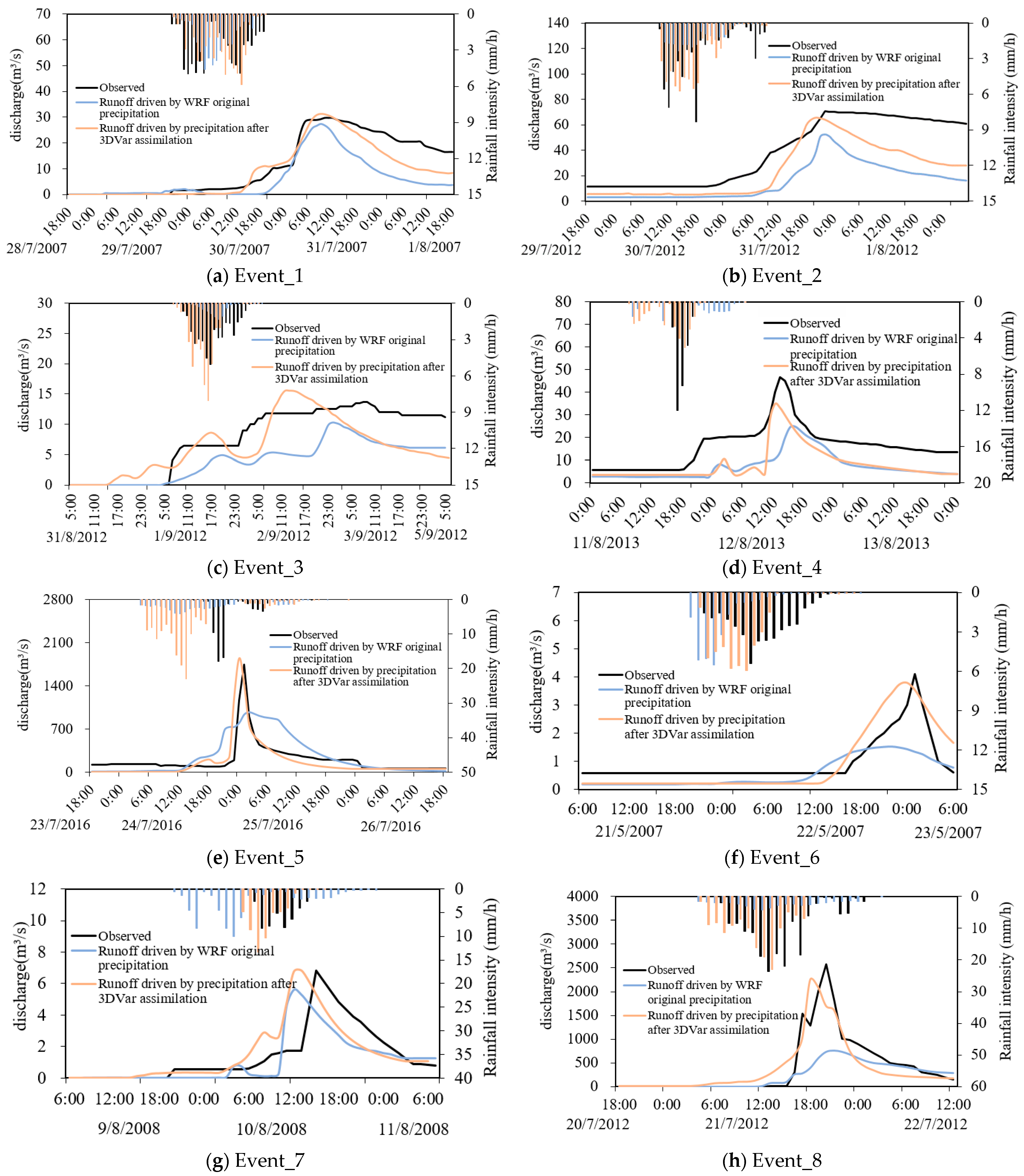
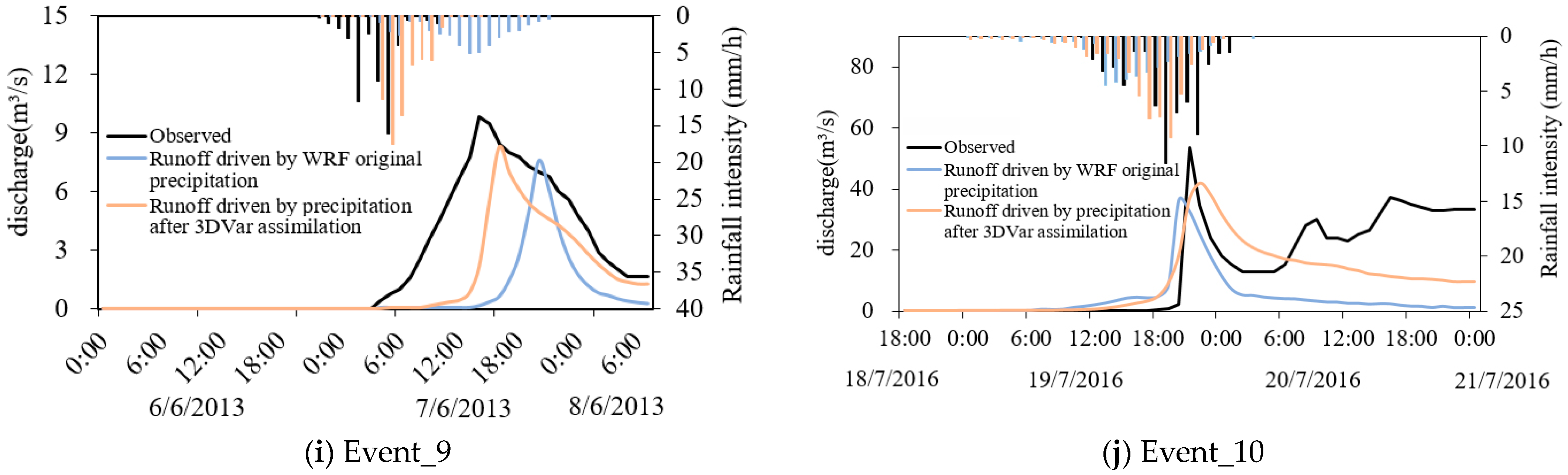
The runoff forecasting results of the WRF-Hydro model are highly dependent on the quality of the precipitation-driven data. To evaluate the effect of the 3Dvar data assimilation on the runoff forecasting through the WRF/WRF-Hydro coupled system, we compared the runoff forecast results from the WRF-Hydro model driven by the WRF precipitation forecasts before and after assimilation, as illustrated in Figure 7. These results were compared with the runoff processes observed at the catchment outlet.

The accuracy of the WRF-Hydro runoff forecast was closely linked to the precipitation-driven data. The precipitation and runoff forecast results of the Zijingguan and Fuping Basins driven by the WRF/WRF-Hydro coupled system forecast precipitation before and after assimilation are compared in Figure 7. By using the forecast precipitation data after the assimilation of radar and GTS data to drive the WRF-Hydro model, the runoff forecast results become more consistent with the observed flow process compared to those before the data assimilation. Specifically, the peak flows of the 10 flood processes before the data assimilation were smaller than the observed ones, whereas the forecast values after the data assimilation significantly increased. This improvement is attributed to the assimilation of radar and GTS data, which leads to more accurate cumulative and hourly precipitation intensities that closely resemble the observed precipitation values. Therefore, the runoff forecast results improved after the data assimilation. However, the flood processes of Event_3, Event_4, and Event_10 take a longer time to recede than those of Event_5, Event_6, Event_7, Event_8, and Event_9. As can be seen in Figure 7, the WRF-Hydro model performs better for flood processes with steep rise, steep fall, and fast receding, while there are larger errors for flood processes with a base flow or that are slow receding in the early stage. In addition, there are still uncertainties in the peak flow and peak time of the events with small precipitation intensity, long duration, and slow water recession, resulting in a fluctuation of the forecast runoff process, such as Event_3 and Event_4. Although data assimilation technology provides more accurate input for the simulation and forecasting of hydrological processes, runoff and precipitation are nonlinearly related. The complexity of the model structure and parameter calibration process influence runoff forecasting. For instance, even though Event_3 precipitation has the most uniform distribution in time and space, the precipitation process after the assimilation changed, with a higher hourly peak precipitation than that observed, thereby leading to more uneven precipitation intensity on the time scale and the fluctuation of the flood process of Event_3 after data assimilation.

In general, the WRF/WRF-Hydro coupled system can well reproduce the hourly runoff process of the basin during the study period. Considering that the WRF precipitation forecast was far lower than the actual precipitation, the forecasted runoff was also lower than the observed runoff at the catchment outlet. However, the assimilation of radar and GTS data brings the overall WRF precipitation forecast closer to the actual precipitation, which is significantly higher than the WRF precipitation forecast. The forecasted runoff results are also far greater than the forecasted flow without assimilation, and the forecasted flood peaks are closer to the observed peaks. To further demonstrate the impact of data assimilation on runoff forecasting,

Table 10. Evaluation indices of the WRF-Hydro runoff forecasts driven by WRF precipitation forecast before and after 3Dvar assimilation.

Event ID	Forecast Flow before Assimilation				Forecast Flow after Assimilation
	NSE	Rf (%)	Rv (%)	T (h)	NSE	Rf (%)	Rv (%)	T (h)
1	0.48	−8.17	−47.86	1	0.85	5.15	−18.52	1
2	0.18	−25.98	−60.37	0	0.70	−7.39	−37.46	2
3	0.25	−24.65	−46.99	8	0.51	13.41	−17.67	20
4	0.09	−47.21	−56.01	−3	0.39	−25.43	−49.67	1
5	0.46	−44.29	24.74	−1	0.71	6.38	−18.27	1
6	0.33	−62.98	−37.31	3	0.48	−7.22	−0.41	1
7	0.33	−17.91	−18.84	4	0.62	0.62	7.18	1
8	0.43	−70.43	−42.19	−1	0.76	−13.01	−5.37	2
9	0.03	−23.15	−71.14	−2	0.51	−16.16	−47.18	−2
10	0.10	−31.74	−68.63	1	0.56	−21.24	−29.33	−1
Mean value	0.27	−35.65	−42.46	1	0.61	−6.49	−21.67	3

shows the NSE, R_f, R_v, and T values driven by different forecasted precipitation values before and after data assimilation.

Table 10 shows that after the assimilation of the 10 flood processes, R_f decreased by 3.02–57.42%, R_v decreased by 6.34–39.30%, and the NSE increased by 0.15–0.52; hence, improvement is evident. In terms of R_f, the degrees of improvement are the most obvious for Event_4, Event_5, Event_6 and Event_8, with R_f being improved by 21.78, 37.91, 55.76, and 57.42%, respectively. Combined with the analysis of precipitation forecast improvement through data assimilation, the RMSEs of the accumulated precipitation after data assimilation for Event_4, Event_5, Event_6 and Event_8 are 1.48, 0.38, 0.42 and 2.62 lower than that before data assimilation, and the CSI/RMSE values are 43.48, 52.58, 27.80, and 18.83% higher than those before data assimilation, respectively. Overall, the improvement in precipitation was relatively large and significantly impacted the flood peak.

Nevertheless, the degree of improvement was nonlinear. Data assimilation improves the accuracy of precipitation forecasts, thereby improving the runoff forecast results of land surface hydrological models. The extent of improvement in the precipitation forecast by data assimilation cannot determine the extent of improvement in the runoff forecast. For example, the precipitation RMSE of Event_7 and Event_9 improved by 84.70 and 83.10%, respectively, after assimilation. These were the greatest improvements among the 10 storms events; however, the runoff forecast results did not significantly improve after assimilation. After the data assimilation, R_f of Event_7 precipitation decreased by 17.30%, R_v decreased by 11.65%, and the NSE increased by 0.29; R_f of Event_9 precipitation decreased by 6.99%, R_v decreased by 23.95%, and the NSE increased by 0.48.

The analysis revealed that the WRF-Hydro runoff forecast accuracy mainly depends on two aspects. On the one hand, the precipitation forecast accuracy of the WRF model is related to the driving data and precipitation distribution type. On the other hand, for precipitation with an uneven spatial-temporal distribution, an imperfect precipitation forecast indirectly affects the flood forecast; however, this may be related to different flood processes, such as flood process complexity, flood magnitude, soil water content, and whether there is a base flow in the early stage. Therefore, data assimilation is not the only factor affecting runoff forecasting, and even with improved rainfall forecasting, there is room for improvement.

4.3. Real-Time Runoff Forecasts Updated by Using LSTM Deep Learning

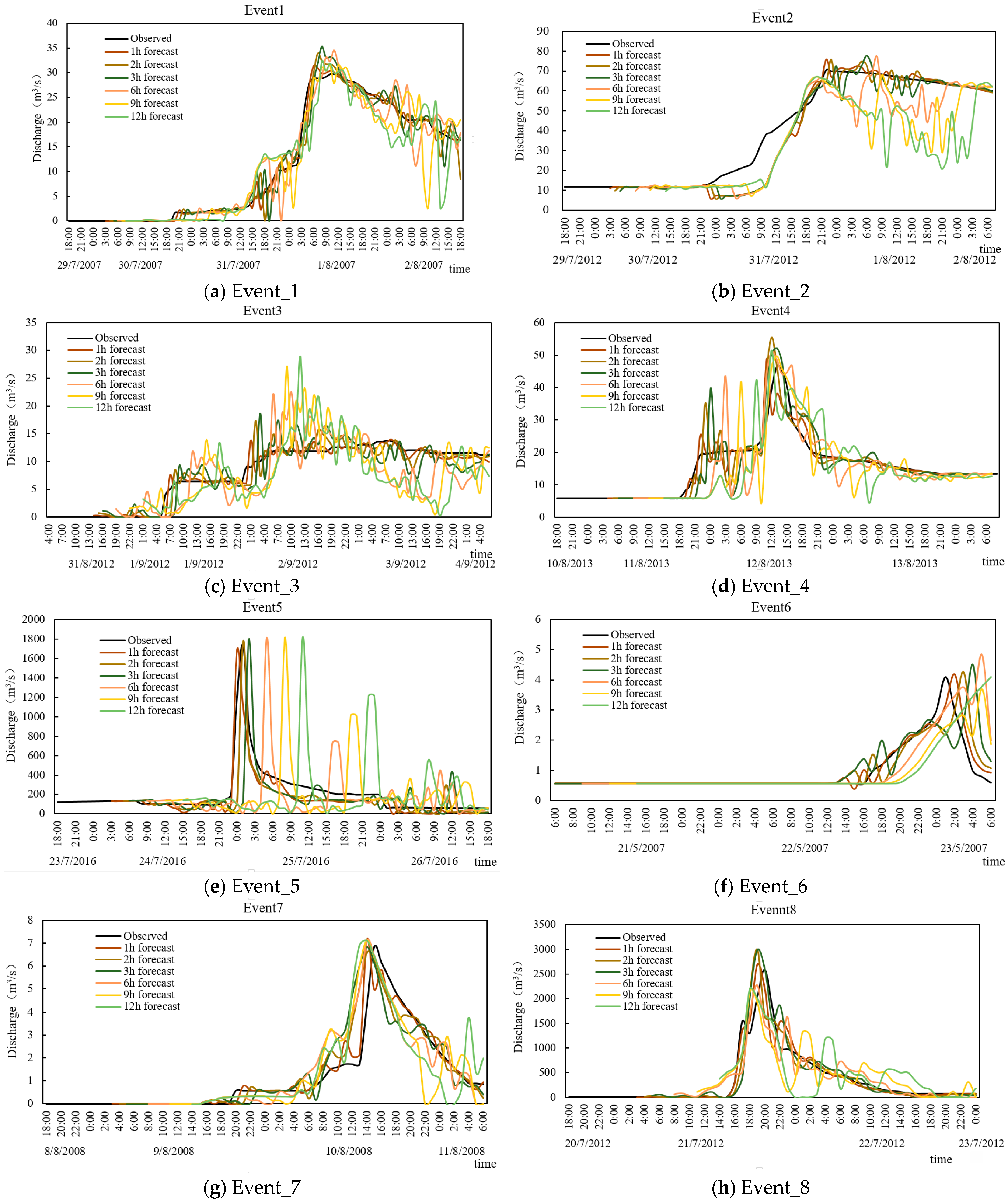
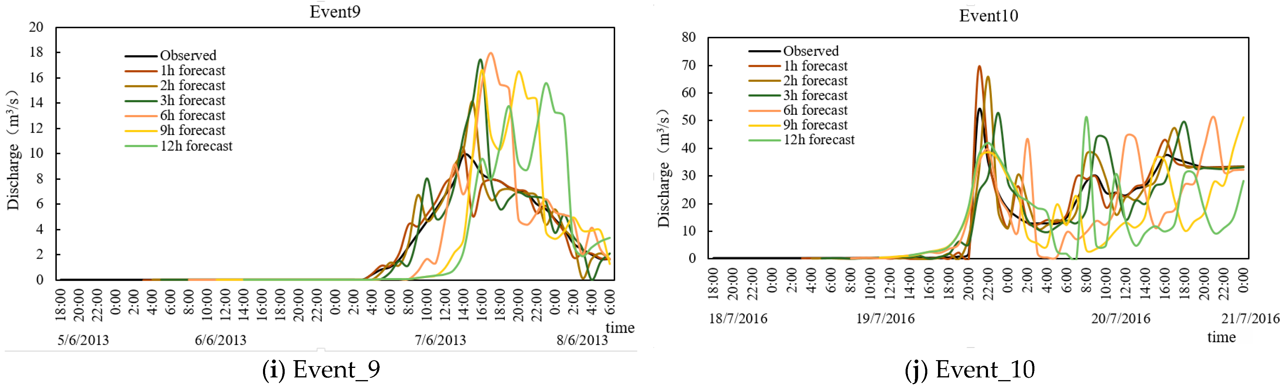
Using the forecasted precipitation after the 3Dvar data assimilation, the LSTM model was used to correct the forecast errors of the WRF/WRF-Hydro coupled system. The real-time runoff forecast results with forecast lead time of 1, 2, 3, 6, 9, and 12 h for the 10 typical flood processes are shown in Figure 8.

Figure 8 shows hydrographs of the forecasted results and actual observations of the 10 storm events with different forecast lead times. The LSTM model performed well in the real-time correction of runoff forecasting, especially for a lead time of 1 h. For a lead time of 3 h, the forecasting results of the runoff process were close to the actual values. For a lead time greater than 6 h, the degree of improvement due to real-time correction on runoff forecasting of the coupled system decreased markedly, while the forecasting fluctuation increased; however, the peak flow and flood volume did not increase or decrease significantly. This is because with the extension of the forecast lead time, the correlation between the forecast errors decrease, and it is difficult for the LSTM model to accurately learn the characteristics of the forecast errors of the coupled system.

Figure 9 illustrates the NSE statistics of the real-time runoff forecasts with different lead times for the 10 storm events. Compared with the runoff forecasting results before correction, the LSTM model significantly improved the accuracy of the runoff forecasting. For the forecasting results with a lead time of 1 h, the NSE is greater than 0.70. With the extension of the lead time, the ability of the real-time correction to improve the runoff forecasting of the coupled system gradually declines. The NSE attenuation rate is calculated according to the percentage change of the NSE values for different lead times compared to those for a lead time of 1 h. With LSTM, for Event_1, the attenuation rate of the runoff forecast is 5.10% for a lead time of 6 h and 10.20% for a lead time of 12 h; for Event_6, the attenuation rate of the runoff forecast is 13.48% for a lead time of 6 h and 33.71% for a lead time of 12 h. Runoff forecasts of the other events showed similar trends. As a real-time correction method for runoff errors, the LSTM model was used to forecast the value of the future time based on historical data. The forecasting results are closely related to the historical data; therefore, if a strong correlation exists between the error series, the error–correction effect is more significant.

Table 11. Evaluation indices for real-time runoff forecasts with different lead times updated by LSTM.

Event ID	Forecast Lead Time	NSE	Rf (%)	Rv (%)	T (h)	Event ID	Forecast Lead Time	NSE	Rf (%)	Rv (%)	T (h)
1	Before LSTM Updating	0.85	5.15	−18.52	1	6	Before LSTM Updating	0.48	−7.22	−0.41	1
	1 h	0.99	5.78	−0.29	3		1 h	0.79	1.84	−8.06	1
	2 h	0.97	14.4	0.71	2		2 h	0.53	3.73	−8.71	2
	3 h	0.96	19.02	3.4	1		3 h	0.21	9.68	−4.6	3
	6 h	0.93	16.2	2.55	1		6 h	−0.07	88.8	7.01	5
	9 h	0.9	6.12	0.25	2		9 h	0.17	−9.74	−23.98	3
	12 h	0.88	8.72	−3.41	1		12 h	−0.46	0	−11.81	4
2	Before LSTM Updating	0.70	−7.39	−37.46	2	7	Before LSTM Updating	0.62	0.62	7.18	1
	1 h	0.90	7.41	−9.55	0		1 h	0.91	4.66	2.92	1
	2 h	0.90	7.36	−8.71	1		2 h	0.84	−3.42	7.39	1
	3 h	0.89	9.95	−8.29	8		3 h	0.7	−0.12	6.71	1
	6 h	0.81	9.8	−12.42	10		6 h	0.73	4.21	6.44	1
	9 h	0.67	−4.01	−17.66	11		9 h	0.62	4.32	1.99	1
	12 h	0.5	−4.85	−18.47	2		12 h	0.54	4.48	4.85	1
3	Before LSTM Updating	0.51	13.41	−17.67	20	8	Before LSTM Updating	0.76	−13.01	−5.37	2
	1 h	0.97	2.89	−0.56	10		1 h	0.89	4.38	1.94	1
	2 h	0.91	26.21	0.22	28		2 h	0.8	15.9	−1.1	1
	3 h	0.79	36.39	−1.55	27		3 h	0.78	15.85	5.2	1
	6 h	0.36	63.73	−6.96	20		6 h	0.77	−11.86	−0.83	1
	9 h	0.11	98.07	3.47	21		9 h	0.61	−16.58	0.46	2
	12 h	0.17	110.88	25.14	18		12 h	0.59	−14.93	0.26	2
4	Before LSTM Updating	0.39	−25.43	−49.67	1	9	Before LSTM Updating	0.51	−16.16	−47.18	−2
	1 h	0.87	5.08	−5.29	2		1 h	0.95	5.69	−0.07	0
	2 h	0.78	19.15	−4.38	1		2 h	0.92	43.25	3.59	1
	3 h	0.75	11.86	−4.38	0		3 h	0.77	75.22	7.37	2
	6 h	0.61	9.16	−11.09	1		6 h	0.37	82.45	9.67	3
	9 h	0.57	6.49	−15.17	0		9 h	0.05	68.81	11	2
	12 h	0.43	10.73	−17.57	1		12 h	−0.04	58.28	7.28	8
5	Before LSTM Updating	0.71	6.38	−18.27	1	10	Before LSTM Updating	0.56	−21.24	−29.33	−1
	1 h	0.75	−3.65	−30.58	1		1 h	0.95	29.28	4.18	0
	2 h	0.63	2.42	−35.65	0		2 h	0.81	23.06	3.92	1
	3 h	−0.15	3.6	−34.2	1		3 h	0.74	−1.18	1.82	2
	6 h	−0.85	4.25	−31.93	4		6 h	0.56	−4.01	−11.08	24
	9 h	−1.08	4.45	−28.24	7		9 h	0.55	−4.22	−18.6	27
	12 h	−1.35	4.57	−26.28	10		12 h	0.38	−3.76	−25.08	11

lists the evaluation indices for the real-time runoff forecasts with different lead times updated by the LSTM. It can be seen that after introducing the LSTM model into the WRF/WRF-Hydro coupled system, the forecasting accuracy of each flood is significantly improved. Specifically, after adding the real-time correction, the fitting of the discharge hydrograph is better, and the NSE is also greatly improved. The NSE values of the forecasting correction results for a lead time of 1 h for all 10 storm events are between 0.75 and 0.99, and the average NSE is 0.90. The correlation between the peak flow and flood volume is good, and the forecasting results are very close to the observations, which shows that the introduction of the LSTM model can increase the flood forecast accuracy. As the lead time increases to 12 h, the NSE is between −0.46 and 0.88, and the average NSE is 0.16, while the correlation between the peak flow and flood volume is poor. Until a lead time of 6 h, the forecast accuracy decreases slowly, while still having a good forecast correction effect. When the lead time is greater than 6 h, the forecast accuracy decreases rapidly, with R_f in all events except Event_10 being within the range of (−10%, 10%). The LSTM model for a lead time of 3 h has relatively high accuracy, with R_f in most events being within the range of (−20%, 20%); however, there are exceptions, for example, for Event_3 and Event_9, R_f of the forecasted values for a lead time of 3 h are 36.39 and 75.22%, respectively. In general, R_f and R_v are low in the runoff forecast for lead times of 0–3 h. However, because the forecast discharge hydrograph fluctuates greatly with the lead time extension, the peak flow and flood volume do not show obvious trends with longer forecast lead times.

5. Discussion

(1) Base flow

The comparison of the WRF precipitation forecast results driving the WRF-Hydro forecast runoff before and after assimilation reveals that the WRF model that assimilates GTS and radar reflectivity is more suitable for coupling with the land hydrological model WRF-Hydro, and the WRF/WRF-Hydro coupled system based on data assimilation shows better forecasting ability in reproducing the flood processes in the Daqing Basin. However, some problems remain, such as base flow. Figure 7 shows that there are obvious base flows in the early precipitation stages in Event_2, Event_4, Event_5, and Event_6. In this study, the base flow module was closed because the bucket model assumes a one-way direct connection between deep groundwater runoff and river channel, which easily causes additional river inflow and is not suitable for short-term forecasting [45]. In semi-humid and semi-arid regions, there are seasonal river channels, and groundwater recharge may not reach the river network; therefore, the bucket model performs poorly in terms of base flow [46]. In addition, in northern China, river water seeps into the soil aquifer for recharge, which is not reflected in the current bucket model. Although the base flow module was not used in this study, it can be used to adjust the proportion of the base flow in the river flow [47]. The lack of a basic flow module also leads to relatively small flood peaks and volumes. In combination with Table 10, under the same conditions, the NSE of Event_2 is 0.18 before assimilation and 0.70 after assimilation; the NSE of Event_4 is 0.09 before assimilation and 0.39 after assimilation; the NSE of Event_5 is 0.46 before assimilation and 0.71 after assimilation; and the NSE of Event_6 is 0.33 before assimilation and 0.48 after assimilation. Although the lack of a basic flow module may lead to instability in the model, improving the precipitation forecast results through data assimilation improves the accuracy of the runoff forecast to a certain extent, indicating that the model is credible. This can be optimized by combining a more practical and physically-based base flow model with the WRF-Hydro model to forecast the deep groundwater recharge in the semi-humid and semi-arid areas, or by extending the warm-up time and conducting long-term forecasting.

(2) LSTM correlation

Table 11 shows that with an increase in lead time, the LSTM model has a poor forecasting effect on events with small peak flows and a better forecasting ability for those with large peak flows. For example, for Event_6 involving a small peak flow, the NSE of the LSTM for a lead time of 3 h is 0.21, the NSE for a lead time of 6 h is −0.07, and the NSE for a lead time of 12 h is −0.46; for Event_8 involving a large peak flow, the NSE of the LSTM for a lead time of 3 h is 0.78, the NSE for a lead time of 6 h is 0.77, and the NSE for a lead time of 12 h is 0.59. There may be two reasons for these unsatisfactory forecasting results. One is the poor correlation of historical runoff errors and the other is the small number of training set samples; therefore, the evaluation indices are contingent. For example, prior to the occurrence of rainfall in the statistical period, there have been many rainfall episodes in Event_5. From 1 May to 24 July 2016, the area rainfall in the Fuping Basin was 340.52 mm, and from 19 July to 22 July 2016, there was a flood process with high rainfall intensity and long duration, with a flood peak of 581 m³/s. Therefore, at the time of occurrence of Event_5, there was a large base flow in the basin, and the soil moisture was relatively saturated, thereby being extremely prone to triggering floods. On 25 July 2016, the highest flood peak reached 1740 m³/s. Therefore, during the period of precipitation generation, the change of flow in Event_5 was affected by stronger factors other than precipitation, such as the lateral flow of runoff, soil moisture or other confluence conditions. Data under the influence of multiple factors led to unsatisfactory LSTM prediction. The NSE of runoff forecasting for Event_5 for a lead time of 3 h is −0.15, the NSE of runoff forecasting for a lead time of 6 h is −0.85, and the NSE of runoff forecasting for a lead time of 12 h is −1.35.

This study involves some limitations. For example, the prediction accuracy of the utilized LSTM deep learning model must be improved when the prediction period exceeds 6 h. In the next step, LSTM can be combined with wavelet transform or BP neural network methods to develop multiple-model joint optimization methods and improve the stability and accuracy of the coupled prediction system. Simultaneously, when defining the LSTM network architecture, the implementation of the multifactor input classification task can be considered by setting the dimensions of the input data to different sizes.

6. Conclusions

Based on the numerical atmospheric model WRF and its land surface hydrological model WRF-Hydro, this study constructed an atmosphere–hydrology coupled system for precipitation–runoff forecasting. Hourly 3DVar data assimilation was adopted to improve precipitation forecasting by the WRF model. On this basis, the improved precipitation forecasts were subsequently used to drive the WRF-Hydro model. In combination with the LSTM model for real-time updating, runoff forecasting based on the WRF/WRF-Hydro coupled system was performed. The effect of data assimilation in improving the WRF forecast precipitation as well as its effect in enhancing the forecast runoff through the coupled system was evaluated. The performance of LSTM was also assessed in correcting the forecast error of the runoff output from WRF-Hydro.

The results showed that it was difficult for the WRF model to accurately forecast the exact time and intensity of precipitation. The CSI/RMSE range of the original forecasts for the 10 storm events was 0.0345–0.6390, which improved to 0.0495–0.9750 after 3Dvar data assimilation. Meanwhile, the runoff forecasting results are highly dependent on the quality of the precipitation data. Data assimilation improved the runoff forecasting results to varying degrees. The runoff error of the 10 storm events was reduced, with the relative error of peak flow (R_f) decreasing by 3.02–57.42%, the relative error of flood volume (R_v) decreasing by 6.34–39.30%, and the NSE increasing by 0.15–0.52.

With the involvement of LSTM, the runoff forecasting accuracy could be significantly improved. LSTM could accurately correct the forecast process of runoff for a lead time of 1 h. The NSE values of the 10 flood events were between 0.75 and 0.98, and the average NSE was 0.90. Peak flow and flood volume were in good agreement with the observations. The runoff forecast for a lead time of 3 h was relatively stable, with peak flow and flood volume being generally reliable. However, for lead times greater than 6 h, the forecasting accuracy decreased rapidly. With the help of 3Dvar assimilation and deep learning correction, storm events with more uniform distributions and more consistent correlations in the historical runoff errors can be better predicted by the WRF/WRF-Hydro coupled system.

References

- Quenum, G.M.L.D.; Arnault, J.; Klutse, N.A.B.; Zhang, Z.; Kunstmann, H.; Oguntunde, P.G. Potential of the Coupled WRF/WRF-Hydro Modeling System for Flood Forecasting in the Ouémé River (West Africa). Water 2022, 14, 1192. [Google Scholar] [CrossRef]
- Varlas, G.; Papadopoulos, A.; Papaioannou, G.; Dimitriou, E. Evaluating the Forecast Skill of a Hydrometeorological Modelling System in Greece. Atmosphere 2021, 12, 902. [Google Scholar] [CrossRef]
- Giannaros, C.; Dafis, S.; Stefanidis, S.; Giannaros, T.M.; Koletsis, I.; Oikonomou, C. Hydrometeorological analysis of a flash flood event in an ungauged Mediterranean watershed under an operational forecasting and monitoring context. Meteorol. Appl. 2022, 29, e2079. [Google Scholar] [CrossRef]
- Hamill, T.M. Performance of Operational Model Precipitation Forecast Guidance during the 2013 Colorado Front-Range Floods. Mon. Weather Rev. 2012, 142, 2609–2618. [Google Scholar] [CrossRef]
- Kryza, M.; Werner, M.; Waszek, K.; Dore, A.J. Application and evaluation of the WRF model for high-resolution forecasting of rainfall—A case study of SW Poland. Meteorol. Z. 2013, 22, 595–601. [Google Scholar] [CrossRef] [PubMed]
- Barker, D.M.; Huang, W.; Guo, Y.; Bourgeois, A.J.; Xiao, Q.N. A Three-Dimensional Variational Data Assimilation System for MM5: Implementation and Initial Results. Mon. Weather Rev. 2004, 132, 897–914. [Google Scholar] [CrossRef]
- Skamarock, W.C.; Klemp, J.B. A time-split nonhydrostatic atmospheric model for weather research and forecasting applications. J. Comput. Phys. 2008, 227, 3465–3485. [Google Scholar] [CrossRef]
- Lewis, J.M.; Derber, J.C. The use of adjoint equations to solve a variational adjustment problem with advective constraints. Tellus A Dyn. Meteorol. Oceanogr. 2022, 37, 309–322. [Google Scholar] [CrossRef]
- Dimet, F.L.; Talagrand, O. Variational algorithms for analysis and assimilation of meteorological observations: Theoretical aspects. Tellus Ser. A-Dyn. Meteorol. Oceanol. 1986, 38A, 97–110. [Google Scholar] [CrossRef]
- Kalman, R.E. A New Approach to Linear Filtering and Prediction Problems. J. Basic Eng. 1960, 82, 35–45. [Google Scholar] [CrossRef]
- Sugimoto, S.; Crook, N.A.; Sun, J.; Xiao, Q.; Barker, D.M. An Examination of WRF 3DVAR Radar Data Assimilation on Its Capability in Retrieving Unobserved Variables and Forecasting Precipitation through Observing System Simulation Experiments. Mon. Weather Rev. 2009, 137, 4011–4029. [Google Scholar] [CrossRef]
- Sun, J.; Flicker, D.W.; Lilly, D.K. Recovery of Three-Dimensional Wind and Temperature Fields from Simulated Single-Doppler Radar Data. J. Atmos. Sci. 1991, 48, 876–890. [Google Scholar] [CrossRef]
- Sun, J.; Crook, N.A. Dynamical and Microphysical Retrieval from Doppler Radar Observations Using a Cloud Model and Its Adjoint. Part I: Model Development and Simulated Data Experiments. J. Atmos. 1998, 55, 835–852. [Google Scholar] [CrossRef]
- Lam, M.; Fung, J.C. Model Sensitivity Evaluation for 3DVAR Data Assimilation Applied on WRF with a Nested Domain Configuration. Atmosphere 2021, 12, 682. [Google Scholar] [CrossRef]
- Neyestani, A.; Gustafsson, N.; Ghader, S.; Mohebalhojeh, A.R.; Körnich, H. Operational convective-scale data assimilation over Iran: A comparison between WRF and HARMONIE-AROME. Dyn. Atmos. Oceans. 2021, 95, 101242. [Google Scholar] [CrossRef]
- Sokol, Z.; Zacharov, P. Nowcasting of precipitation by an NWP model using assimilation of extrapolated radar reflectivity. Q. J. R. Meteorol. Soc. 2012, 138, 1072–1082. [Google Scholar] [CrossRef]
- Tai, S.; Liou, Y.; Sun, J.; Chang, S.; Kuo, M. Precipitation Forecasting Using Doppler Radar Data, a Cloud Model with Adjoint, and the Weather Research and Forecasting Model: Real Case Studies during SoWMEX in Taiwan. Weather Forecast. 2011, 26, 975–992. [Google Scholar] [CrossRef]
- Davolio, S.; Silvestro, F.; Gastaldo, T. Impact of Rainfall Assimilation on High-Resolution Hydrometeorological Forecasts over Liguria, Italy. J. Hydrometeorol. 2017, 18, 2659–2680. [Google Scholar] [CrossRef]
- Mazzarella, V.; Maiello, I.; Capozzi, V.; Budillon, G.; Ferretti, R. Comparison between 3D-Var and 4D-Var data assimilation methods for the simulation of a heavy rainfall case in central Italy. Adv. Sci. Res. 2017, 14, 271–278. [Google Scholar] [CrossRef]
- Lagasio, M.; Silvestro, F.; Campo, L.; Parodi, A. Predictive Capability of a High-Resolution Hydrometeorological Forecasting Framework Coupling WRF Cycling 3DVAR and Continuum. J. Hydrometeorol. 2019, 20, 1307–1337. [Google Scholar] [CrossRef]
- de Souza, P.M.M.; Vendrasco, E.P.; Saraiva, I.; Trindade, M.; de Oliveira, M.B.L.; Saraiva, J.; Dellarosa, R.; de Souza, R.A.F.; Candido, L.A.; Sapucci, L.F.; et al. Impact of Radar Data Assimilation on the Simulation of a Heavy Rainfall Event Over Manaus in the Central Amazon. Pure Appl. Geophys. 2022, 179, 425–440. [Google Scholar] [CrossRef]
- Cáceres, R.; Codina, B. Radar data assimilation impact over nowcasting a mesoscale convective system in Catalonia using the WRF model. Tethys J. Mediterr. Meteorol. Climatol. 2018, 15, 3–17. [Google Scholar] [CrossRef]
- Zhu, B.; Pu, Z.; Putra, A.W.; Gao, Z. Assimilating C-Band Radar Data for High-Resolution Simulations of Precipitation: Case Studies over Western Sumatra. Remote Sens. 2022, 14, 42. [Google Scholar] [CrossRef]
- Hochreiter, S.; Schmidhuber, J. Long Short-Term Memory. Neural Comput. 1997, 9, 1735–1780. [Google Scholar] [CrossRef]
- Hu, C.; Wu, Q.; Li, H.; Jian, S.; Li, N.; Lou, Z. Deep Learning with a Long Short-Term Memory Networks Approach for Rainfall-Runoff Simulation. Water 2018, 10, 1543. [Google Scholar] [CrossRef]
- Kratzert, F.; Klotz, D.; Brenner, C.; Schulz, K.; Herrnegger, M. Rainfall–runoff modelling using Long Short-Term Memory (LSTM) networks. Hydrol. Earth Syst. Sci. 2018, 22, 6005–6022. [Google Scholar] [CrossRef]
- Zhang, D.; Hølland, E.S.; Lindholm, G.; Ratnaweera, H. Hydraulic modeling and deep learning based flow forecasting for optimizing inter catchment wastewater transfer. J. Hydrol. 2018, 567, 792–802. [Google Scholar] [CrossRef]
- Qiu, Q. Precipitation Nowcasting Based on Blending Weather Radar with Numerical Weather Model and Its Application; China Institute of Water Resources and Hydropower Research: Beijing, China, 2020. [Google Scholar]
- Wang, W. Atmospheric-Hydrologic Simulations in the Mixed Runoff Generation Area Based on the Fully Coupled WRF/WRF-Hydro Modeling System; Hohai University: Nanjing, China, 2021. [Google Scholar]
- Qie, X.; Zhu, R.; Yuan, T.; Wu, X.; Li, W.; Liu, D. Application of total-lightning data assimilation in a mesoscale convective system based on the WRF model. Atmos. Res. 2014, 145, 255–266. [Google Scholar] [CrossRef]
- Tong, W.; Li, G.; Sun, J.; Tang, X.; Zhang, Y. Design Strategies of an Hourly Update 3DVAR Data Assimilation System for Improved Convective Forecasting. Weather Forecast. 2016, 31, 1673–1695. [Google Scholar] [CrossRef]
- Liu, J.; Bray, M.; Han, D. Exploring the effect of data assimilation by WRF-3DVar for numerical rainfall prediction with different types of storm events. Hydrol. Process. 2013, 27, 3627–3640. [Google Scholar] [CrossRef]
- Liu, J.; Wang, J.; Pan, S.; Tang, K.; Li, C.; Han, D. A real-time flood forecasting system with dual updating of the NWP rainfall and the river flow. Nat. Hazards 2015, 77, 1161–1182. [Google Scholar] [CrossRef]
- Tian, J.; Liu, J.; Wang, J.; Li, C.; Yu, F.; Chu, Z. A spatio-temporal evaluation of the WRF physical parameterisations for numerical rainfall simulation in semi-humid and semi-arid catchments of Northern China. Atmos Res. 2017, 191, 141–155. [Google Scholar] [CrossRef]
- Tian, J.; Liu, J.; Yan, D.; Li, C.; Yu, F. Numerical rainfall simulation with different spatial and temporal evenness by using a WRF multiphysics ensemble. Nat. Hazard. Earth Syst. Sci. 2017, 17, 563–579. [Google Scholar] [CrossRef]
- Lorenc, A.C. Analysis methods for numerical weather prediction. Q. J. R. Meteorol. Soc. 1986, 112, 1177–1194. [Google Scholar] [CrossRef]
- Tian, J.; Liu, J.; Yan, D.; Li, C.; Chu, Z.; Yu, F. An assimilation test of Doppler radar reflectivity and radial velocity from different height layers in improving the WRF rainfall forecasts. Atmos. Res. 2017, 198, 132–144. [Google Scholar] [CrossRef]
- Senatore, A.; Mendicino, G.; Gochis, D.J.; Yu, W.; Yates, D.N.; Kunstmann, H. Fully coupled atmosphere—Hydrology simulations for the central Mediterranean: Impact of enhanced hydrological parameterization for short and long time scales. J. Adv. Model Earth Syst. 2015, 7, 1693–1715. [Google Scholar] [CrossRef]
- Silver, M.; Karnieli, A.; Ginat, H.; Meiri, E.; Fredj, E. An innovative method for determining hydrological calibration parameters for the WRF-Hydro model in arid regions. Environ. Model Softw. 2017, 91, 47–69. [Google Scholar] [CrossRef]
- Liu, Y.; Liu, J.; Li, C.; Yu, F.; Wang, W.; Qiu, Q. Parameter Sensitivity Analysis of the WRF-Hydro Modeling System for Streamflow Simulation: A Case Study in Semi-Humid and Semi-Arid Catchments of Northern China. Asia Pac. J. Atmos. Sci. 2021, 57, 451–466. [Google Scholar] [CrossRef]
- Hornik, K.; Stinchcombe, M.; White, H. Multilayer feedforward networks are universal approximators. Neural Netw. 1989, 2, 359–366. [Google Scholar] [CrossRef]
- de Villiers, J.; Barnard, E. Backpropagation neural nets with one and two hidden layers. IEEE Trans. Neural Netw. 1993, 4, 136–141. [Google Scholar] [CrossRef]
- Stefanidis, S.; Dafis, S.; Stathis, D. Evaluation of Regional Climate Models (RCMs) Performance in Simulating Seasonal Precipitation over Mountainous Central Pindus (Greece). Water 2020, 12, 2750. [Google Scholar] [CrossRef]
- Dai, Y.; Zeng, X.; Dickinson, R.E.; Baker, I.; Bonan, G.B.; Bosilovich, M.G.; Denning, A.S.; Dirmeyer, P.A.; Houser, P.R.; Niu, G.; et al. The Common Land Model. Bull. Am. Meteorol. Soc. 2003, 84, 1013–1024. [Google Scholar] [CrossRef]
- Osuri, K.K.; Mohanty, U.C.; Routray, A.; Niyogi, D. Improved Prediction of Bay of Bengal Tropical Cyclones through Assimilation of Doppler Weather Radar Observations. Mon. Weather Rev. 2015, 143, 4533–4560. [Google Scholar] [CrossRef]
- Lahmers, T.M.; Gupta, H.; Castro, C.L.; Gochis, D.J.; Yates, D.; Dugger, A.; Goodrich, D.; Hazenberg, P. Enhancing the Structure of the WRF-Hydro Hydrologic Model for Semiarid Environments. J. Hydrometeorol. 2019, 20, 691–714. [Google Scholar] [CrossRef]
- Arnault, J.; Wagner, S.; Rummler, T.; Fersch, B.; Bliefernicht, J.; Andresen, S.; Kunstmann, H. Role of Runoff–Infiltration Partitioning and Resolved Overland Flow on Land–Atmosphere Feedbacks: A Case Study with the WRF-Hydro Coupled Modeling System for West Africa. J. Hydrometeorol. 2016, 17, 1489–1516. [Google Scholar] [CrossRef]
Figure 1.
Flowchart of the study.
Figure 2.
Location map of the study area.
Figure 3.
Study area with nested configuration of WRF domains at 9, 3, and 1 km resolution.
Figure 4.
Radar data and GTS data assimilation process.
Figure 5.
Schematic diagram of the LSTM deep learning model.
Figure 6.
Accumulations of the WRF precipitation forecasts before and after 3Dvar data assimilation.
Figure 7.
Runoff forecast results driven by the WRF precipitation forecasts before and after 3Dvar data assimilation.
Figure 8.
Real-time runoff forecast results corrected by LSTM driven by WRF forecast precipitation after data assimilation.
Figure 9.
NSE statistics of the real-time runoff forecasts with different lead times for the 10 storm events.