
Effects of Spatial Data Acquisition on Determination of a Gravel-Bed River Geomorphology


Department of Water Engineering, Shahid Bahonar University of Kerman, Kerman 76169-13439, Iran
*
Author to whom correspondence should be addressed.
Water 2023, 15(9), 1719; https://doi.org/10.3390/w15091719
Submission received: 29 March 2023
/
Revised: 23 April 2023
/
Accepted: 26 April 2023
/
Published: 28 April 2023
(This article belongs to the Special Issue Water, Geohazards, and Artificial Intelligence)
Abstract
:Bed irregularities of water bodies play a significant role in many hydraulic and river engineering experiments and models. Accurate measurement of river geomorphology requires great fieldwork effort. Optimizing the dataset size of measured points will reduce the time and costs involved. In this study, the geomorphology of a gravel bed river reach was measured using different spatial acquisition methods. Digital elevation models were created for each measurement method and the volumes of under/overestimation were calculated. The results show that the sampling methods had more effect on the accuracy of the interpolated geomorphology than the density of the measured points. By choosing an optimized sampling method, the measurement efforts decreased to less than 50%, with negligible errors of around 15 m3 and 10 m3 over and underestimation, respectively, in a water body area of around 2200 m2. These findings help to provide more accurate geomorphological data with less effort as inputs for experimental and numerical models to derive better results.
1. Introduction
Detailed and accurate bathymetric measurements of riverbeds are as important as measurements of hydraulic parameters [1,2]. The initial use of riverbed measurements is to evaluate the wetted area, perimeter, hydraulic radius, average water depth, and bed slope, which are the most important parameters in many formulas and models to evaluate the hydraulic parameters of rivers. In addition to these parameters, dense measurements of riverbeds provide useful information about riverbed fluctuations and bedforms. These data are useful for roughness calculation and the lives of aquatic animals, on one hand. On the other hand, they provide spatial and temporal information about the morphological changes, volumes of sediment deposition and erosion, and locations of scour and fill [3,4]. Understanding the volume of transported sediment is important for evaluating the hydro-geomorphological regime of the rivers located downstream of dams in response to the water–sediment regulation schemes, such as the study of [5]. It is also important in cases where there is a reservoir downstream of the river for evaluating the filling rate of the reservoir. Transported sediments increase the filling rate and decrease the reservoir capacity by approximately 1% per year [6,7]. Detailed bathymetry measurements provide useful information about the roles of flow characteristics, turbulence characteristics, and secondary currents in sediment transport under different conditions, which are, at the moment, unknown [8]. Although there are different measurement methods and numerical models and devices for sediment transport measurements, topo-bathymetric surveys are the most accurate method and are useful for model and measurement device calibrations. This method is commonly used for measurements of reservoir capacity and to calculate filling volumes due to sediments [9]. The aforementioned information shows the importance of bathymetric measurements in river engineering, water management, and echo hydraulic applications.
To measure river bathymetry, the height of every point as well as the surface X–Y coordinates of the point are measured. Terrestrial laser scanning, synoptic remote sensing, airborne photogrammetry, and light detection and ranging (LiDAR) provide very dense and spatially distributed point clouds of riverbeds. These devices are applicable in seasonal rivers when there is either no water in the river or shallow clear water [10,11,12]. These devices have a much greater range of errors associated with individual point elevations [13]. In deep rivers or rivers carrying suspended loads, such as Alpine rivers, these devices are not useful and ground-based methods (total station theodolite and RTK-GPS/dGPS) are required [2].
The measured points are used to create a digital elevation model (DEM) of the study area. DEMs are mainly used in fluvial geomorphology research to assess and quantify morphological changes and sediment budgets using repeated topographic surveys [14,15,16,17]. If other parameters are measured, then digital terrain models (DTMs) are created. DTMs are important for many other water-related analyses, such as the distribution of velocity along the river [18], or parameters related to the hydrodynamic processes of aquifer systems, such as the studies of [19,20] as a few examples. DEMs are created based on the idea that the unmeasured areas can be interpolated using the measured points. There are different interpolation methods that affect the accuracy of extracted DEMs, e.g., Delaunay triangulation (DT), inverse distance-weighted function (IDW), kriging, local polynomial, spline, etc. [2]. The aforementioned methods are not only used for bathymetry measurements, but also for calculating the spatial distributions of hydraulic parameters, such as water velocity, shear velocity, etc. For example, kriging can be used as an interpolation method for presenting the spatial distributions of the hydraulic parameters of a gravel-bed river [21]. The quality of the bed fluctuation DEMs affects the output of the flow simulations [22] and accurate volumetric estimations of channel changes [23]. There have been many studies investigating different methods of geostatistical analyses to obtain accurate DEMs from surveyed points [7,13,24,25,26,27]. Erdogan 2009 [28] related DEM quality to three main factors: (i) the accuracy, density, and distribution of the source data; (ii) the interpolation process; and (iii) the characteristics of the surface. For a similar surface and interpolation method, DEM error is also a function of the (i) data point measurement accuracy; (ii) measured point density to represent the surface; and (iii) field survey strategy [29]. The latter two parameters depend on the field sampling strategy.
A dense bed measurement strategy represents the shape of landforms accurately. Dense surveying using ground-based devices is very time-consuming and costly, requires highly qualified personnel, is applicable for reaches with limited vegetation, and, in some cases, is dangerous [2]. Reducing the measured point densities increases errors, especially when the goal of measurement is to evaluate the volume of erosion/deposition or to calculate accurate dimensions of bedforms. To have a balance between point density and accuracy, measurement strategies must be presented. The investigation of different surveying strategies suggested morphological methods based on break lines to improve the accuracy of DEMs [2,13]. Break lines are defined as a topographic break in the cross-section of a slope, such as a bank top, toe slope, or thalweg [2]. Therefore, these methods are based on the initial knowledge of the reach’s topography and differ between various case studies. For deep rivers with unclear water where information about break lines is missing, these methods do not work properly. Therefore, there is a need to introduce a measuring method that is independent of the bed morphology, can be applied under every condition, and has available information about its error.
In all studies, data are measured along discrete or continuous lines. Examples of discrete lines are measurements that are conducted along cross-sections with different intervals of 5 m to more than 100 m [30,31,32]. Another example of discrete lines is measurements along longitudinal sections, which are increasingly being used [18,33]. Continuous lines are also measurements conducted along a serpentine/zigzag path [21,31,34,35]. The interval of the lines is not similar in all studies and differs based on the working load and the required accuracy. Therefore, there is not enough information about the accuracy of each method or the optimum interval for the measured lines. Applying an appropriate surveying method has more effects on the accuracy of the results than the interpolation method [2,13]. On one hand, there is also a gap in the literature regarding which information about the determination of the optimal data-collection strategy is missing [18]. On the other hand, in studies that investigated the effects of sampling strategies and interpolation methods, it has been mentioned that more studies are required to determine if the results can be transferred to other rivers or not [36].
To address these gaps, we focus on the measurement strategies and the corresponding errors. A gravel-bed river reach was selected. River bathymetry was measured in a dense grid and assumed to be a reference riverbed. The novelty of this study is that different methods of measurement, such as zigzag, cross-sectional, and longitudinal measurements, with different intervals were tested. DEMs of the riverbed were created and the volumes of under/overestimations were calculated for each method. The findings of the present study will be useful in (i) determining the optimum method and interval of measurement points, (ii) saving time and money for each measurement campaign, and (iii) having an overview of the approximate errors of the created DEMs in different measurements.
2. Materials and Methods
The selected reach was from a permanent river in northern Iran with a gravel bed. Descriptions of the reach are presented in Table 1. For safety reasons, the maximum water depth and flow velocity in all measured areas were less than 1 m and around 1 m/s, respectively. Owing to the existence of a storage dam upstream of the study reach, there was almost constant discharge in the river during the measurement periods. As a result, the water surface was almost constant during all measurements. Owing to the suspended sediment load, the riverbed was not visible, even at a flow depth of less than 30 cm.
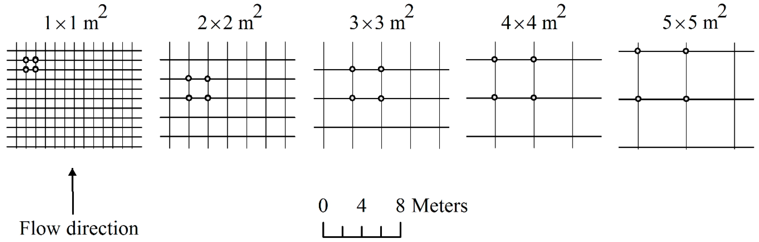
An STS752 6L Sanding theodolite total station with accuracies of 2 s and 2 mm for angle and length readings, respectively, was used to measure the river bathymetry. Therefore, the water depth and velocity did not affect the results. The 3D coordinates of each point were measured in a grid of 1 × 1 m2. Ropes were used along the width of the river to maintain longitudinal intervals. The ropes were marked every 1 m to maintain transverse intervals. It was assumed that the bathymetry obtained from this surveying point cloud represented the riverbed with no error. In this study, 22 different acquisition methods were used in around 10 days. These methods were categorized into 5 groups. The first group included 4 methods in which the dimensions of the measured grids increased from 2 × 2 to 5 × 5 m2 (Figure 1).
If boats are used to measure bathymetries or hydraulic parameters, it is possible that, along the boat path, the interval of measurement points is very small. This occurs when moving-boat acoustic Doppler current profilers (ADCP) are used (e.g., in [21,31,32]). For these devices, the distance between the measured points along the boat path is too close, and the accuracy of measurements depends on the movement of the boat. In the next 3 groups, which contain 14 methods, it is assumed that a moving boat device is used to measure the bathymetry. The scheme of these methods is presented in Figure 2 and Figure 3.
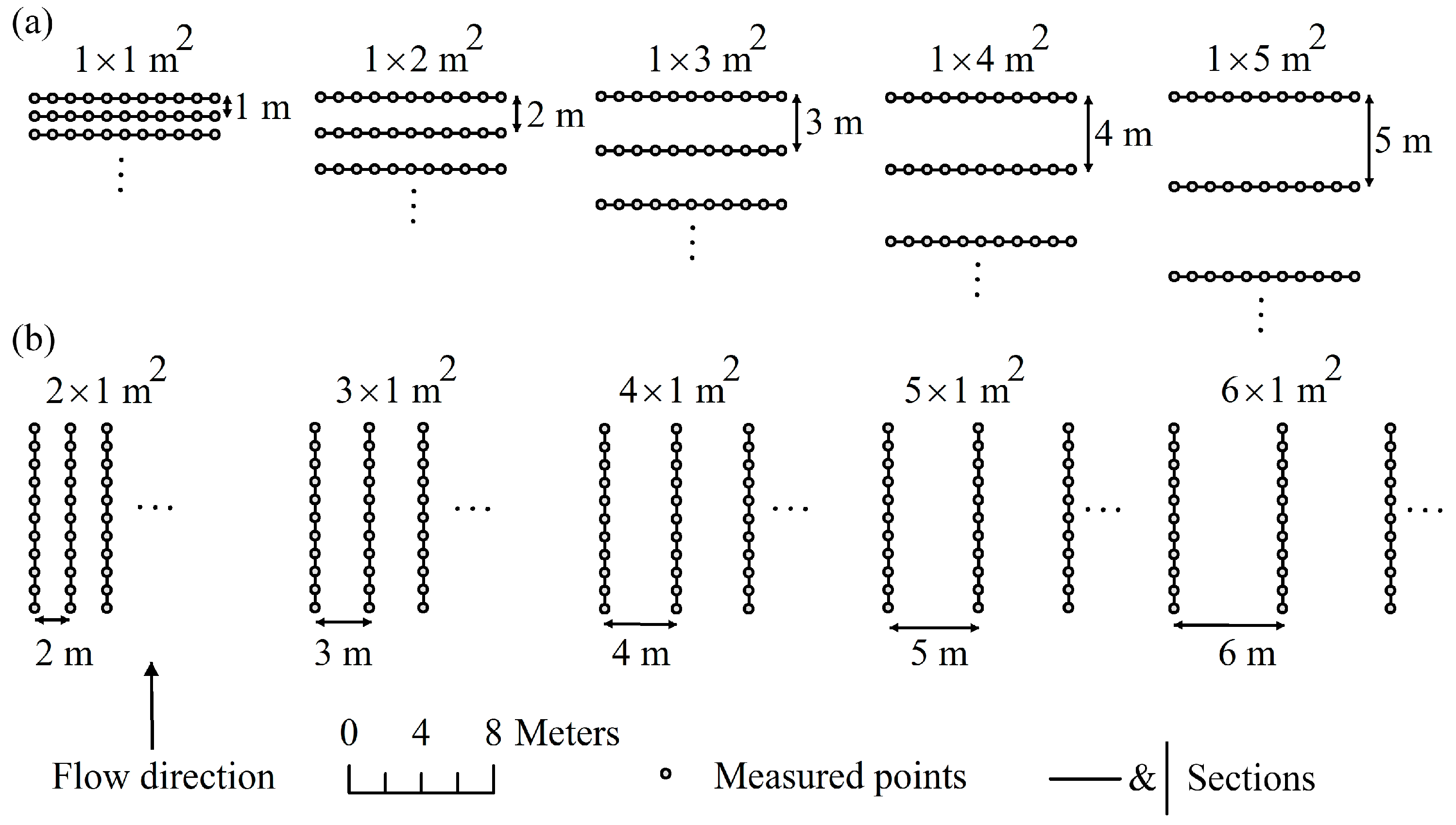
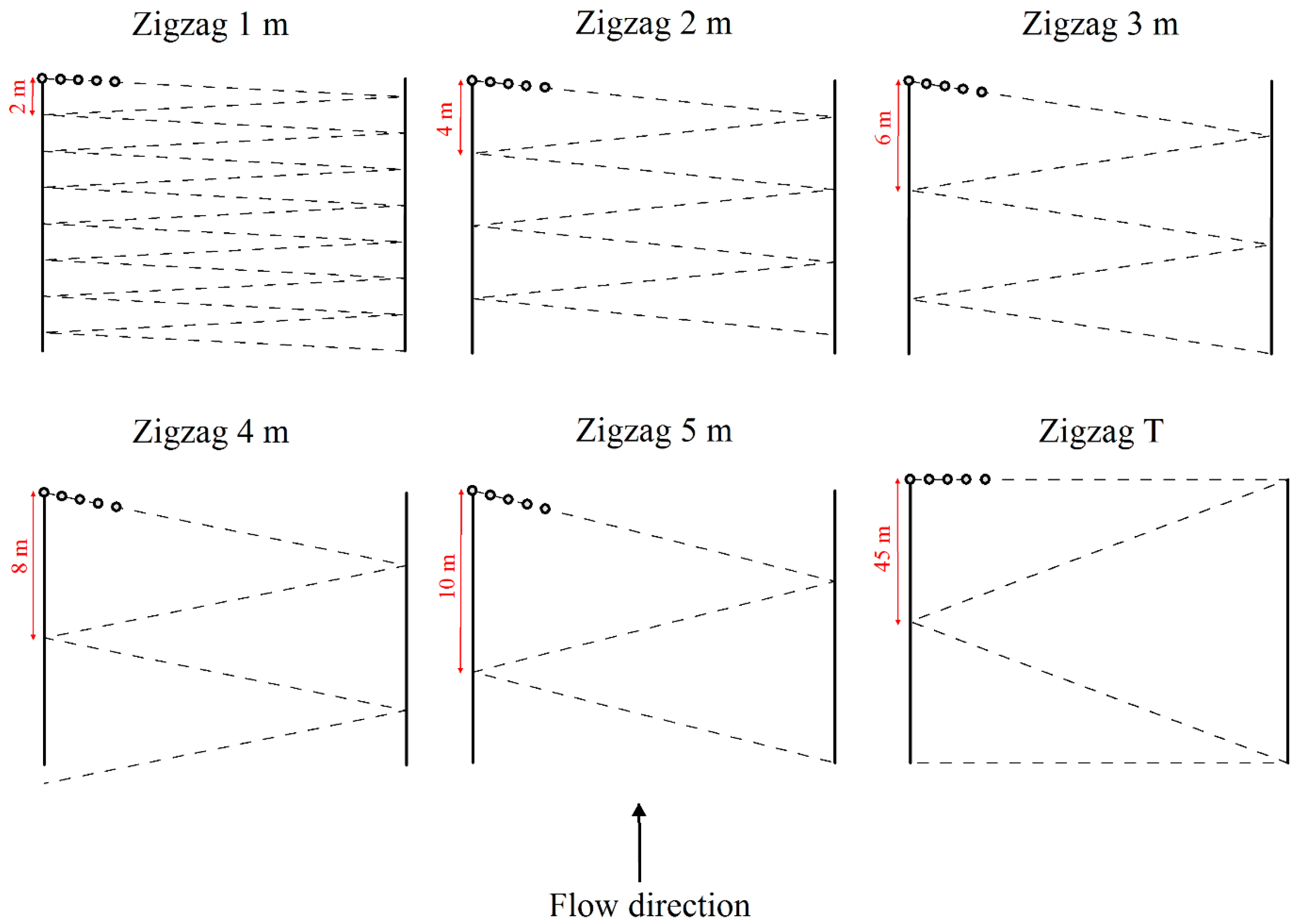
Figure 2a,b shows that the surveying points were measured at cross-sections and longitudinal sections, respectively. The interval of the sections increased from 2 m to 5 m and 2 m to 6 m for the cross- and longitudinal sections, respectively. Zigzag measurements were based on the movements of the boats or the surveyor. The last method for zigzag measurement was independent of the length of the reach—the surveyor starts from a bank, a cross-section is measured, and at the next bank, zigzag movement starts. They continue to half of the river reach and then to the same bank at the ending location of the reach. Then, from that location, a cross-section is measured again. In this study, the measured points along the lines had an interval of around 1 m for all methods in these 3 groups, while in the moving ADCPs, it could reach around 10 cm based on the ADCP type and boat speed. The last group contained 3 methods that could be used when time and safety are more important (Figure 4). To achieve very quick measurements or traditional one-dimensional (1D) modeling applications, cross sections are used to describe river bathymetry [37]. For this purpose, three cross-sections at the upstream, middle, and downstream locations of the reach were chosen. In some cases, one to three additional longitudinal profiles were also measured (Figure 4).
3. Results
3.1. Different Interpolation Methods
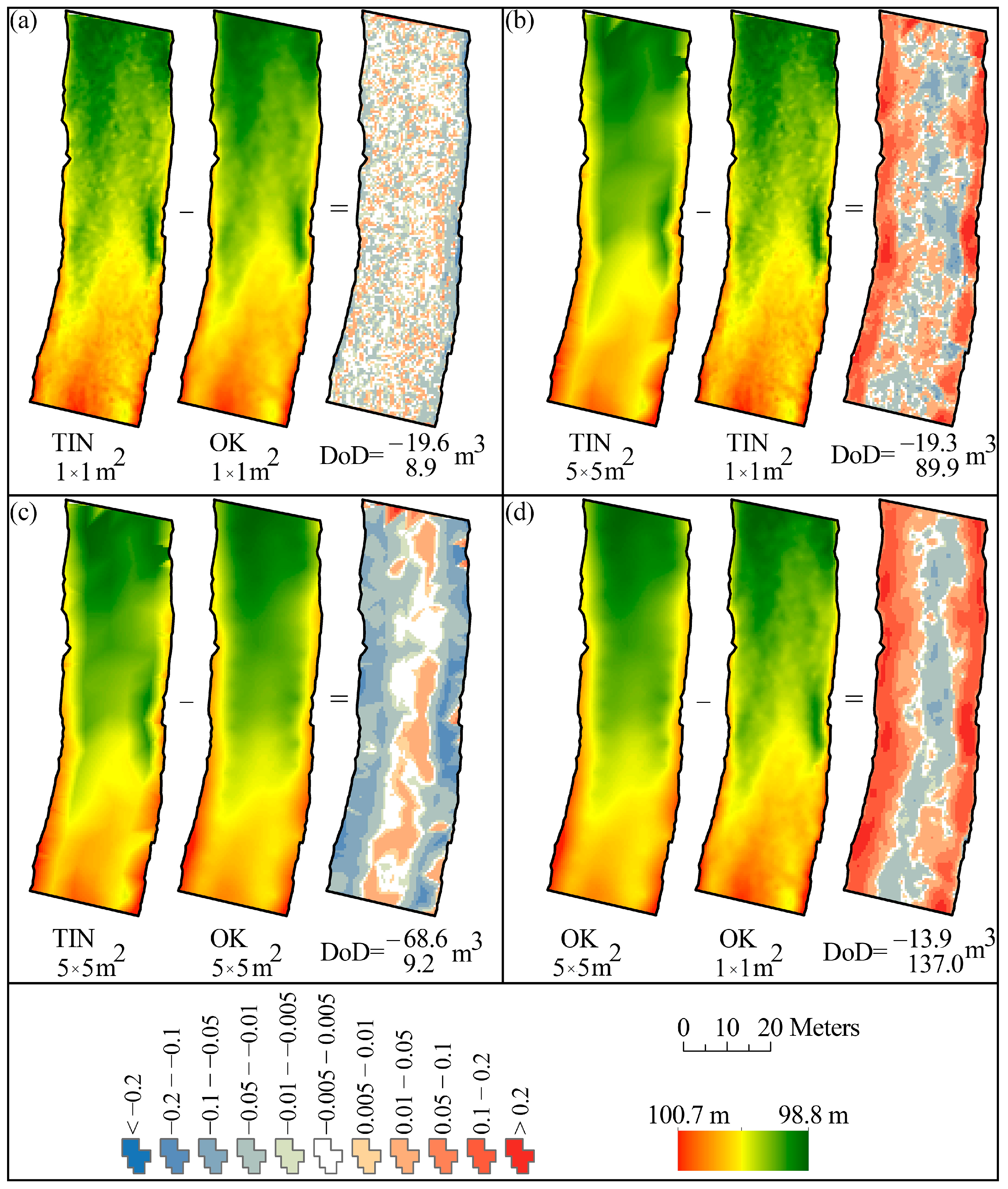
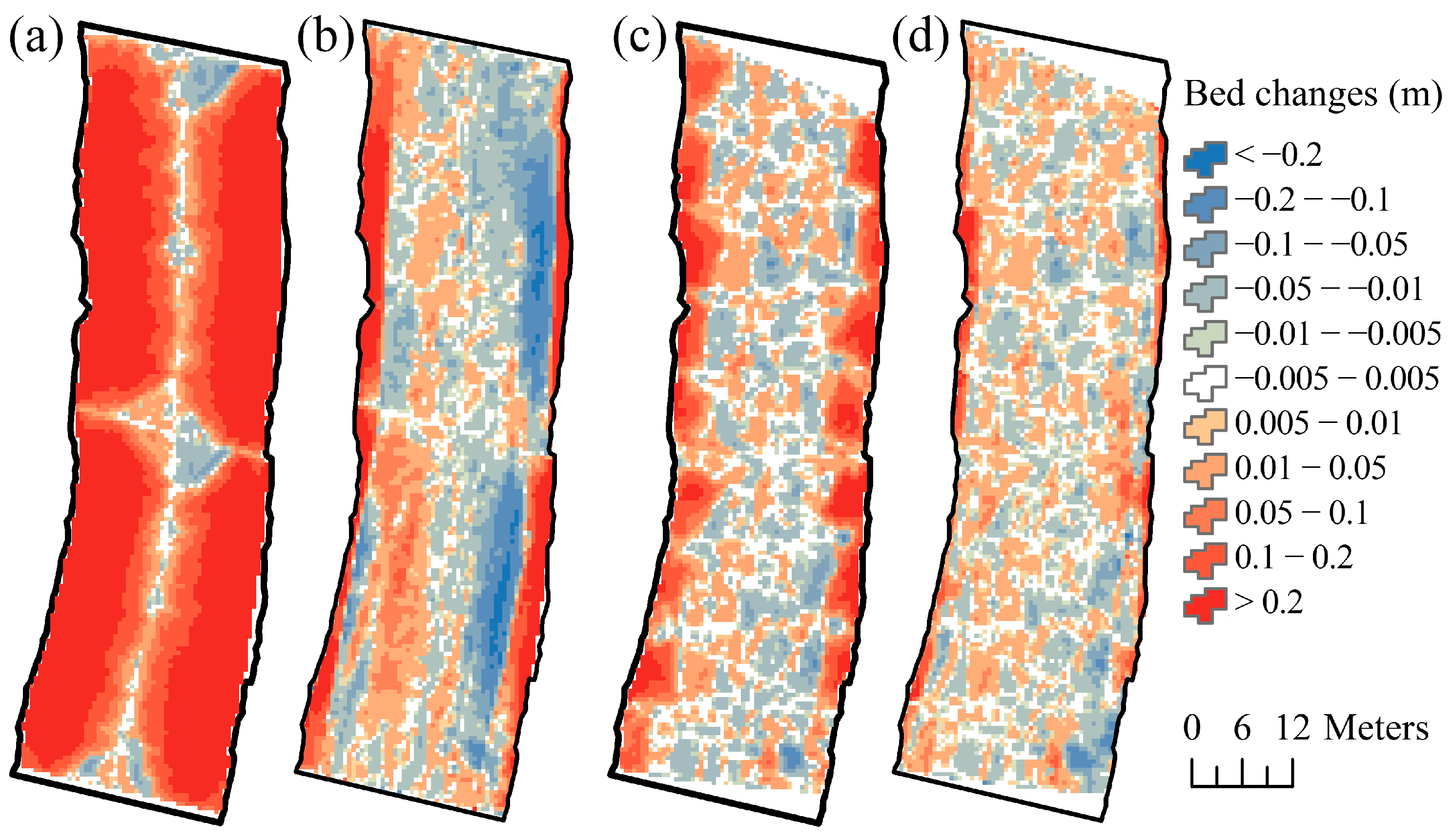
DEMs were created by the interpolation of unmeasured areas in the study reach. The most common and best interpolation methods used in fluvial geomorphology are the triangular irregular network (TIN) and ordinary kriging (OK) [13]. In this study, both methods were used to create DEMs from regular grids of 1 × 1 m2 and 5 × 5 m2. Figure 5 shows the differences between both interpolation methods. Figure 5a shows that, in a dense measurement survey, there was not a dramatic difference between the TIN and OK. By decreasing the density to 5 × 5 m2, OK produced smoother DEMs and performed better than the TIN (Figure 5c). Although the smoothness of a DEM is not the governing parameter, resulting in the lowest difference in the DEM of difference (DoD) is the main parameter. Based on Figure 5b,d, DEMs created by TIN resulted in a lower difference than OK. This shows that TIN was better than OK for grids with lower point density. Therefore, further analysis of the surveying methods was conducted using TINs. The created TIN was then converted to a raster with dimensions of 0.25 m2 using the linear method. The bed topography extracted from the 1 × 1 m2 measurement was considered to be the base map and represented the real morphology of the bed.
3.2. Regular Grid Methods
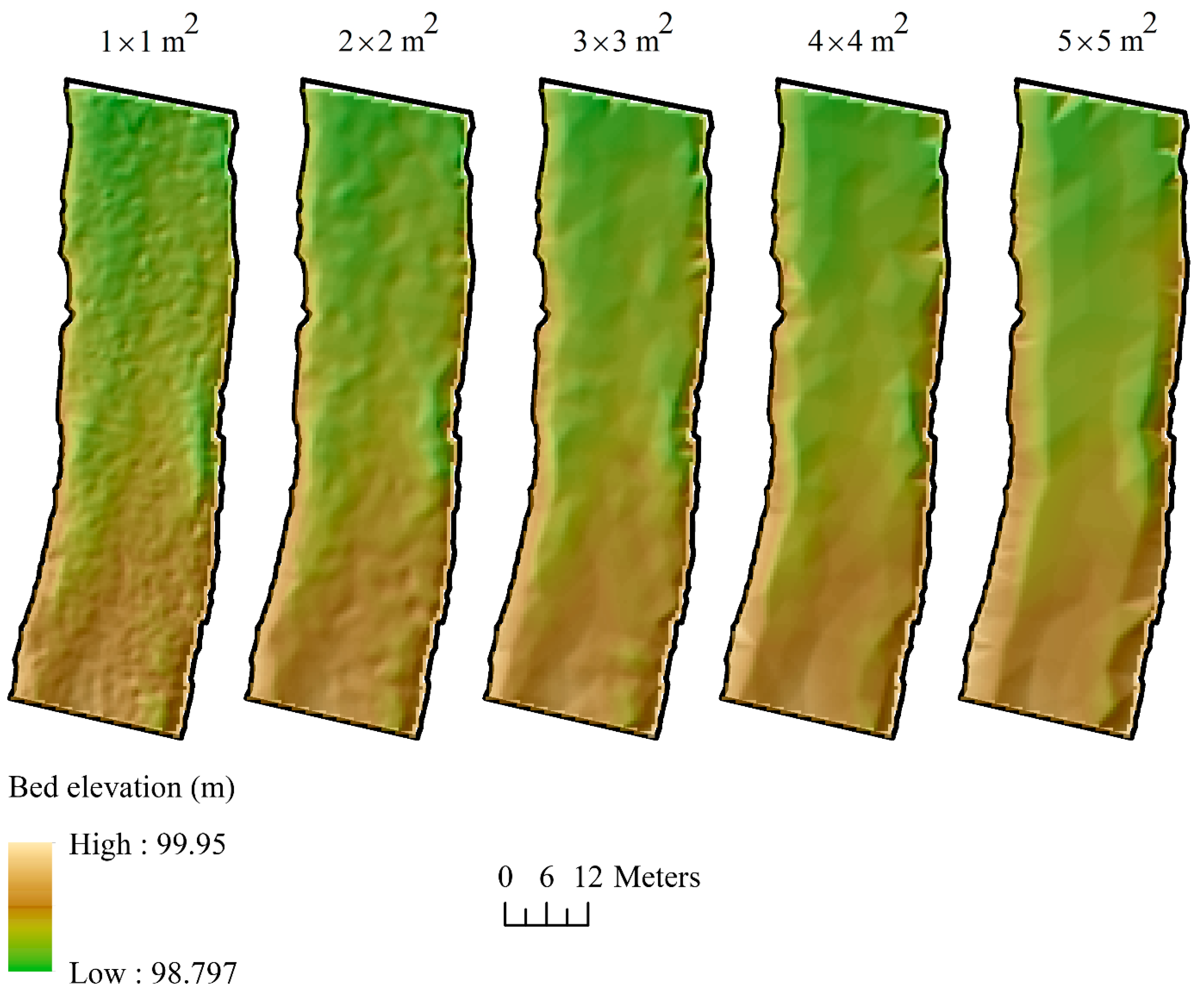
Figure 6 shows that, by reducing the point density, although some details were missing, the overall shape of the riverbed, including the locations of pools, riffles, and bedforms, was still detectable. All DEMs showed that the upstream of the reach had a bed elevation of around 99.9 m and, going downstream, the elevation of the left bank decreased to 99 m. The decrease continued further downstream and reached a value of 98.7 m. There was also a small area of 50 m2 to the right in the upstream part of the reach with an elevation of 99.1 m—all DEMs showed this area very well. Although more details are presented in the 1 × 1 m2 and 2 × 2 m2 grids, the other grids show the area and depth of these locations. Overall, Figure 5 shows that, in the selected gravel-bed river, by decreasing the point density and using wider measurement grids, the overall shape of the riverbed could be measured and erosion and deposition areas were presented. The average elevation of the riverbed was also calculated with some small percentages of errors. However, the pattern of the riverbed was presented properly. The percentages of the errors will be calculated further. The grids presented in Figure 5 are useful when ground-based measurement devices are used.
3.3. Cross and Longitudinal Section Methods
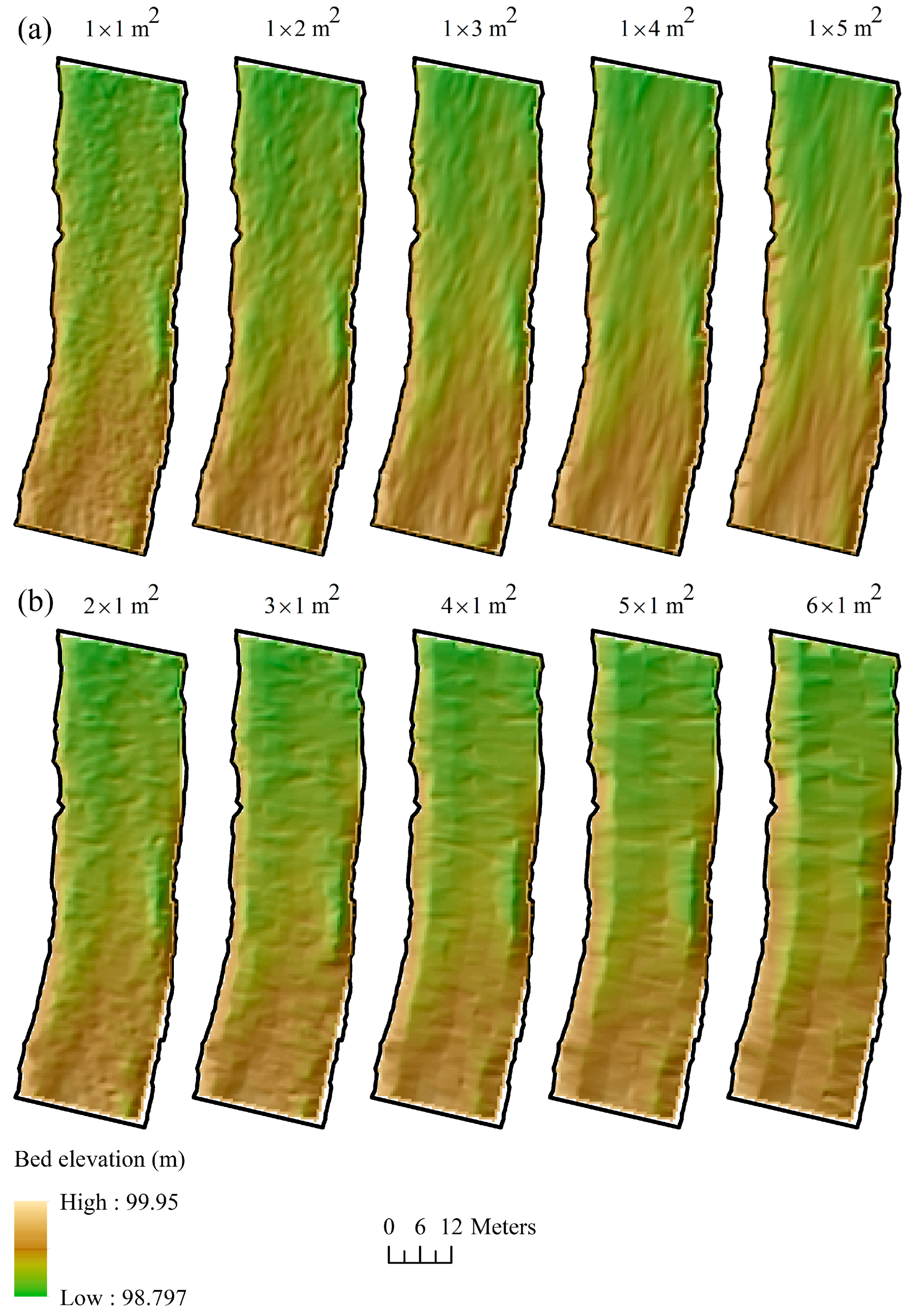
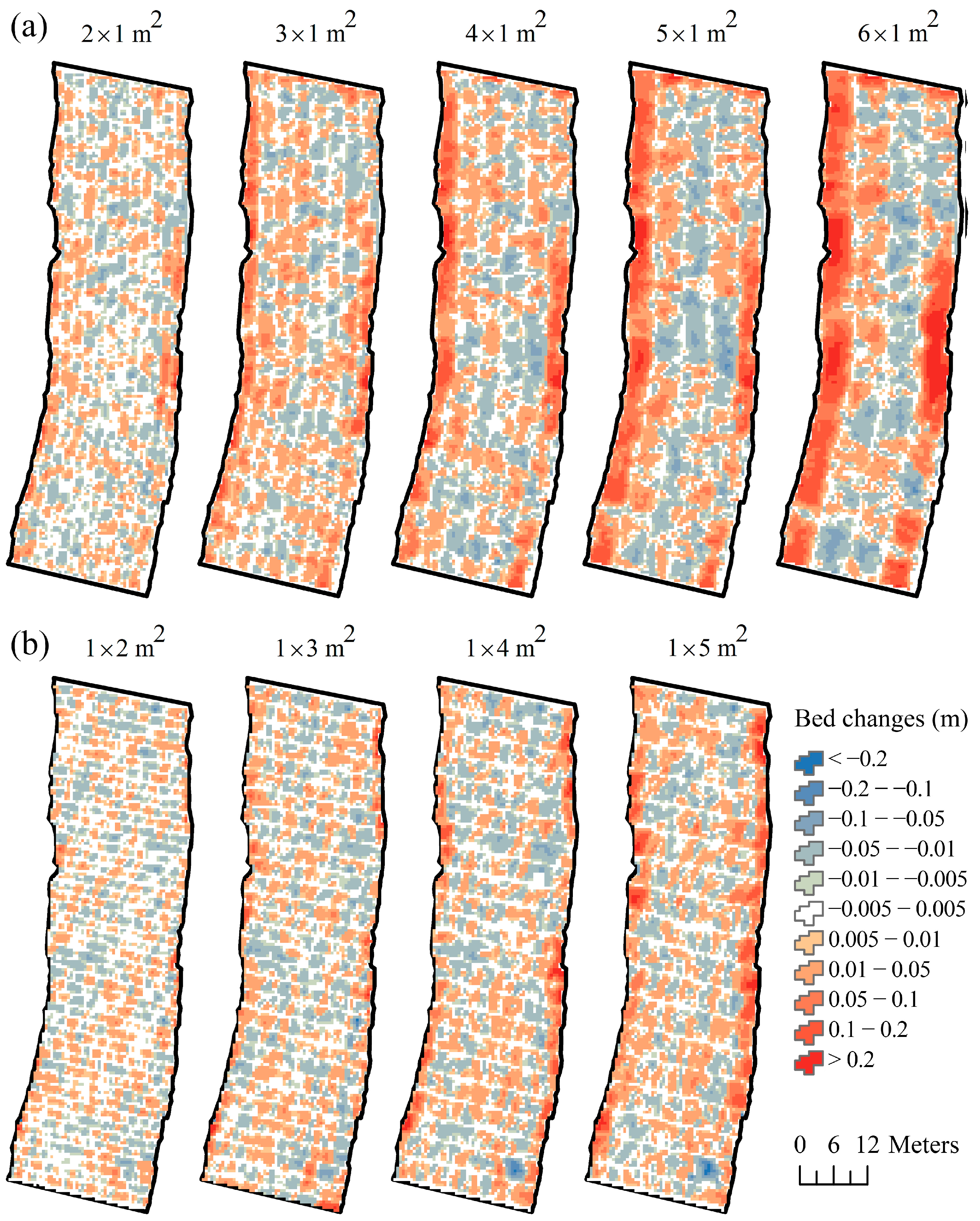
Figure 7a,b shows the extracted DEMs from cross-sectional and longitudinal measurements, respectively. Figure 7a shows that, in the cross-sectional measurements, by increasing the interval to 4 m, details could be presented properly. By increasing the distance of the cross sections to 5 m, some breaks were created, especially in regions near the banks. A similar pattern existed for the 2 and 3 m intervals in the longitudinal measurements. If the distance between the longitudinal sections increased to 4 m or above, fewer details were presented and the created DEM was not very accurate.
3.4. Zigzag Methods
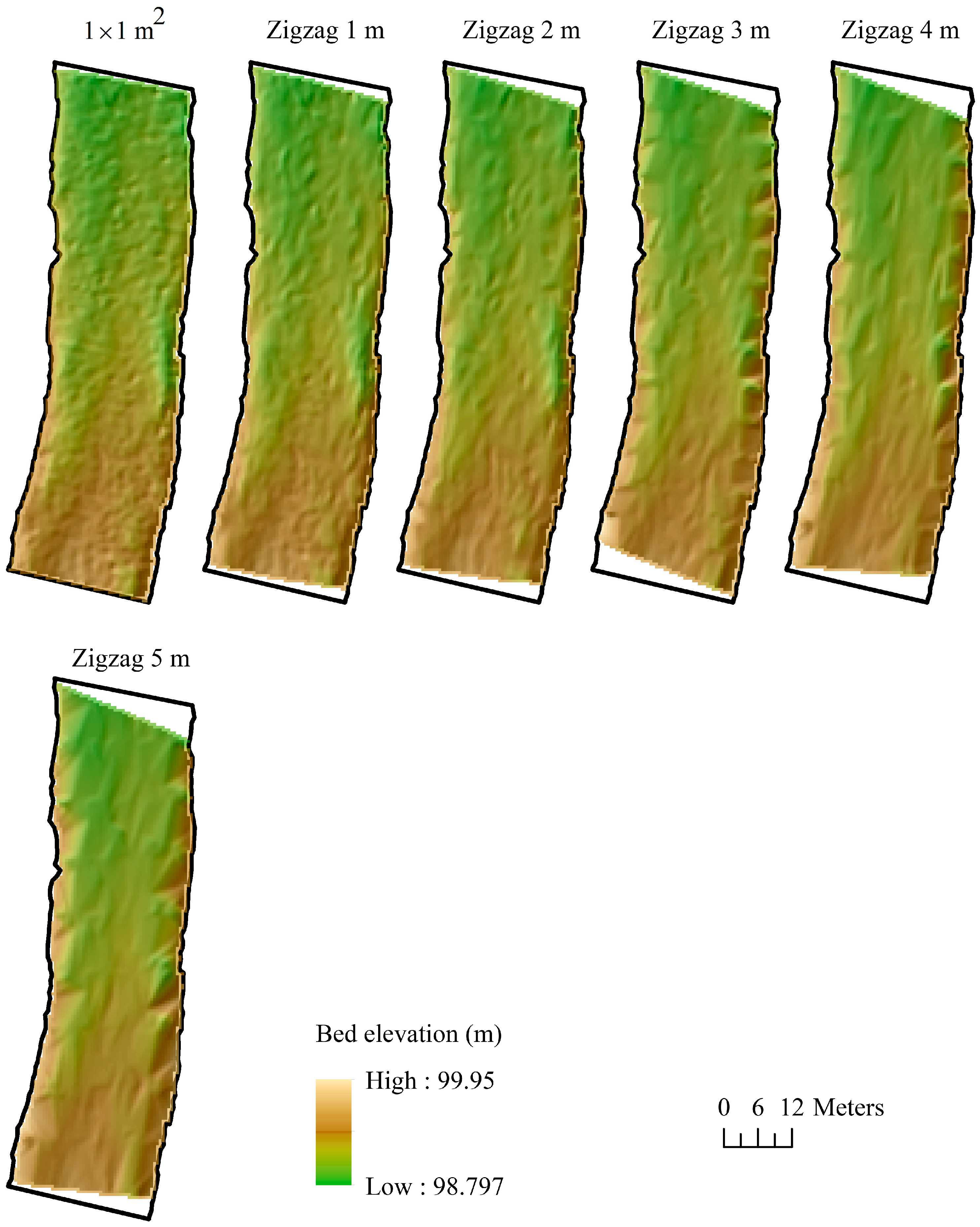
In some locations, such as lakes and wide channels, it is hard to keep the line in a longitudinal or transverse direction because of the long distance between the starting and ending points of each section. To reduce the measurement effort and the measured point density, zigzag measurements were used. The results are presented in Figure 8. Zigzag measurements are very useful, especially when echo sounders and ADCPs are used for bathymetry measurements. Figure 8 shows the accuracy of different zigzag measurement methods. The one-meter zigzag and two-meter zigzag methods showed the details of the riverbed. By increasing the wavelength, fewer details were measured, especially near the banks. For the 3 m zigzag method, small areas near the banks showed more errors. By increasing the wavelength, these areas became larger and extended to the center line of the channel. Apart from that, all zigzag measurements showed their capability to measure the overall details of channel bathymetry.
3.5. Large-Scale Methods
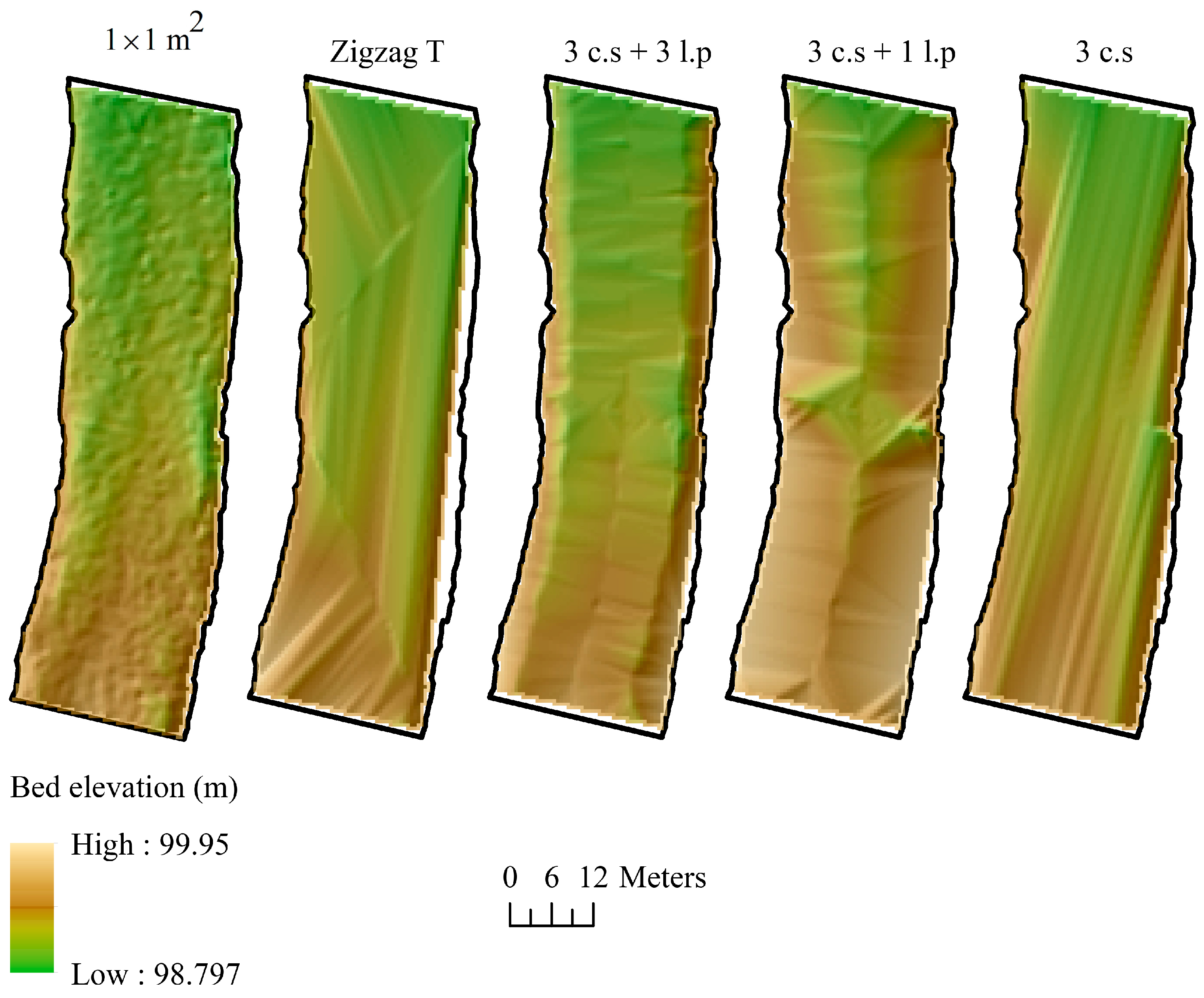
There are other types of measurements when details are less important and large-scale monitoring has more priority. In these cases, the measurements are conducted following cross-sectional methods with large intervals. To check the accuracy of these methods, three cross-sections were measured in the selected reach and the DEM was created using the measured cross-sections. Another method was to measure one to three longitudinal sections in addition to three cross-sections to determine how they improved the accuracy of the results. Another method in Figure 9 was the use of zigzag measurements as a replacement for cross sections and longitudinal lines. It proposed that, not only could the middle part of the channel, but also regions near the banks, be measured. Figure 9 shows that the four methods did not show many details of the riverbed, no bedforms were detected, and the locations of bars or pools and riffles were presented very roughly. The only use of these measurements would be to calculate the slope of a channel and an approximate location of large-scale phenomena with no accurate 3D dimensions. These methods are also used for 1D software calibrations. Among these four methods, three cross-sections in addition to three longitudinal cross-sections seemed to be more accurate and showed more details in comparison with the other three methods.
3.6. Measurement Errors and Durations of Each Method
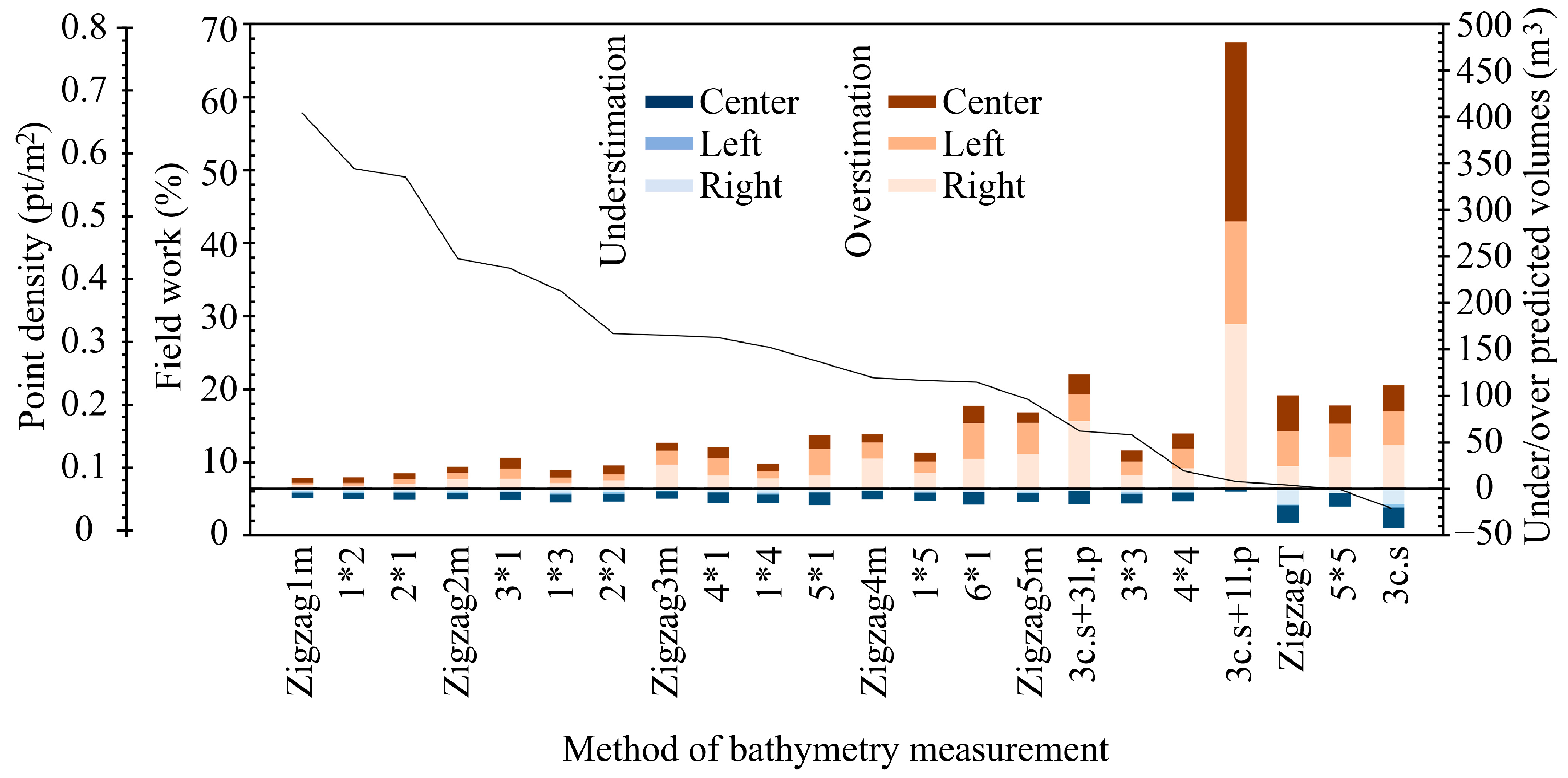
Figure 6, Figure 7, Figure 8 and Figure 9 show the 3D elevation models of the reach using different measurement methods. These figures show how different methods presented the bathymetric details of a gravel-bed river. Although some methods showed enough detail, the estimation of the percentage of error would be necessary. Figure 10 presents the accuracy of each measurement method, as well as the point density and amount of fieldwork required. The 1 × 1 m2 measurement method had a point density of 1.14 points per square meter, with a measurement duration of 10 h. Figure 10 shows that, by using the 1 m zigzag method, the fieldwork decreased to around 60 percent (it took 6 h to conduct measurements). The measurement of only three cross-sections also took 30 min. Figure 10 shows that, although the measurement methods were different, for some methods, the measured point density and fieldwork did not change dramatically. For example, 1 × 2 m2 had similar point density and fieldwork to the 2 × 1 m2 method.
Previous studies used statistical parameters to evaluate the accuracy of each acquisition method [36], but in this study, we used the volumes of the under/overestimation of the riverbed to evaluate the accuracy of each method (Figure 10). This parameter is important in sedimentation studies, where the calculation of the amount of eroded or deposited sediments is important. Figure 10 shows that increasing the point density in some methods did not necessarily decrease the error. The method including three measured cross-sections and one longitudinal profile is a good example of this. Although three cross-sections with one longitudinal section had higher point density than the zigzag method, for a grid of 5 × 5 m2 and three cross-sections, the volumes of overestimation were much higher than those of every other method. Figure 10 also shows that the volumes of overestimation were much higher than the volumes of underestimation. On the other hand, the volumes of overestimation in regions near the banks were similar to the volumes in the central region. Although the right and left bank regions occupied 24 and 17 percent of the whole studied area, respectively, the calculated volumes of errors in these regions were similar to those of the central 59 percent of the reach. Figure 10 shows that increasing the measured points did not necessarily increase the accuracy of the DEMs. Comparing cross-sectional and longitudinal grids showed that cross-sectional grids were more accurate than longitudinal grids. Figure 10 also shows that regular grids had better performance than the longitudinal and cross-sectional measurements, although they could decrease the measurement fieldwork to a greater extent than the other methods.
Figure 11, Figure 12 and Figure 13 show the locations of errors in different methods. Figure 11 shows that, by increasing the grid dimensions, the banks will be overestimated by about 20 cm. The areas of underestimation mostly occurred in the center of the reach, and the maximum depth difference was 20 cm in very small areas.
Figure 12a shows that the longitudinal methods provided good information in the central regions. By increasing the interval between the longitudinal lines, the error increased to more than 20 cm, especially near the banks. Figure 12b shows that all cross-sectional measurement methods had fewer errors eventually when the distance between the two cross-sections increased to 5 m and the fieldwork decreased to 2 h. In this measurement method, the areas where the bed elevation difference was less than 5 mm were larger than those in other methods. The only issue was in some small areas near the banks, which had an error of around 20 cm.
Figure 13a shows that zigzag measurements had small errors, especially with small wavelengths. By increasing the wavelength to 5 m, the errors increased significantly near the banks.
Figure 13b shows that large-scale methods did not provide accurate results. All methods had large areas with errors of more than 20 cm. The method with three cross-sections and one longitudinal section showed overestimation, while the other methods had both overestimated and underestimated areas, with a depth deference of around 20 cm.
4. Discussion
4.1. Interpolation Methods
Figure 5 shows that, for very dense point measurements, there was no difference between the interpolation methods, which was similar to the findings of Bengora et al., 2018 [7]. By decreasing the point density, the quality of the produced DEMs was affected by interpolation methods. For the scattered point density, OK showed smoother DEMs. Other studies also suggested that ordinary kriging (OK) could accurately predict hydraulic features, bathymetry, sediment flux, flow, and process variance in the anisotropic nature of hydraulic structures and channel shapes [18,21,36,38,39]. Although OK presented smoother DEMs, the difference in the DEMs with a 1 × 1 m2 grid indicated the better performance of TINs. These observations are consistent with those of Puente and Bras (1986) [40] and Bengora et al., 2018 [7], who showed that kriging may result in important under or overestimation of the prediction error when the size of a dataset decreases. Other studies also found TINs to be more reliable and well-suited to discontinuous shapes and breaks in slope [41,42]. Figure 5 also shows that TINs performed better than OK for banks with steep slopes. The results support the findings of Heritage et al., 2009 [13] regarding the use of TINs as the best interpolator in fluvial environments. The TIN itself is particularly prone to misrepresenting surface topography when low point density and greater topographic complexity combine [17]. Figure 5 also shows that, for lower density and near banks, TINs did not display the bed very well, but the amount of over/underprediction was less than that of OK. Therefore, the interpolation method affected the accuracy of the results, especially for scattered point densities, which is the opposite of the findings of Heritage et al., 2009 [13], which indicated that the choice of the interpolation algorithm is not as important as the survey strategy, but similar to those of Chaplot et al., 2006 [43] and Yue et al., 2007 [44], which indicated that the interpolation methods influence the accuracy and quality of the produced DEMs.
4.2. Measurement Methods
Previous studies [18,36] expected that a decrease in data density would correspond to an increase in error. The results of the present study show that increasing the number of measured points did not necessarily increase the accuracy of DEMs, which demonstrated the importance of strategy over the point density. Heritage et al., 2009 [13] also indicated that an inappropriate point sampling regime results in errors in surveying.
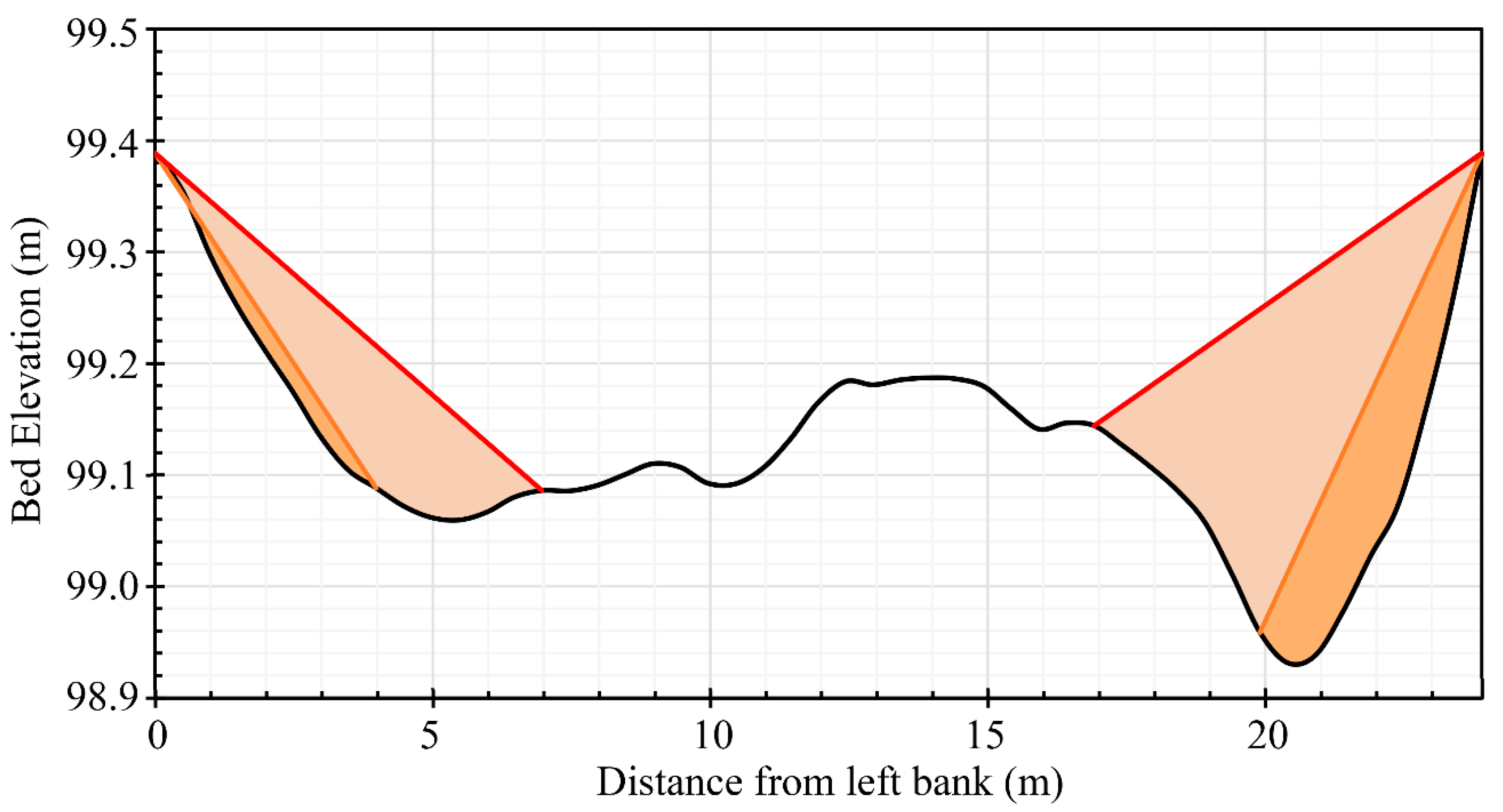
Comparing all measurement methods showed that the overestimation volumes were higher than the underestimation volumes, especially for regions near the banks. High variability in the parameters of riverbanks caused increases in error, not only for bathymetry mapping, but also for other parameters, such as velocity, as described in previous studies [18]. For bathymetry, there was a steep slope in transverse directions in the regions near the banks. Heritage et al., 2009 [13] also found that the greatest error was located at the breaks of slopes and Krüger et al., 2018 [36] found higher errors near the banks. Figure 14 presents a cross section of a riverbed. The black line indicates the real bed and the two color lines are interpolated lines.
Figure 14 shows that, if the measured points were far from the banks, the interpolated values would be higher than the real value of the bed, which is similar to the findings of Bengora et al., 2018 [7]. They also found that the overestimation of the sediment volume in a reservoir was due to the concave shape of the water body, and by decreasing the number of measured points, the overestimated volume of sediments increased. The transverse slope of riverbeds near banks is steep; therefore, increasing the measurement point distance in the transverse direction causes more errors than increasing the distance in the longitudinal direction. Heritage et al., 2009 [13] also reported that there is a relationship between surface topographic variation and DEM error. Therefore, a field survey strategy is very important for mapping topographic variations correctly. The findings of Banjavcic and Schmidt 2018 [18] for velocity mapping can also be explained by Figure 14. They found that the interpolated transect velocities did not match the cross-section velocity trend and consistently underestimated the depth-averaged velocity. Based on Figure 14, the velocity at banks is lower than that in the central channel, opposite to the bathymetry; therefore, the interpolated values would be below the real values for velocities.
In cross-sectional methods, by increasing the distance of the cross-sections to 5 m, some lines were created, especially in regions near the banks. These lines caused under/overestimations based on the elevation difference between the banks and the center of the reach. Banjavcic and Schmidt 2018 [18] also reported that the distance between cross-sections is a significant factor for obtaining a river-reach-scale velocity map. Glenn et al., 2016 [45] concluded that the accuracy of bathymetric data using cross-sectional measurements was not significantly dependent on the transect location or interpolation method, but was highly correlated with transect spacing. They suggested that transects spaced further apart than three times the average bank full width significantly decreased the accuracy of interpolated bathymetric information. Heritage et al., 2009 [13] reported that DEM error is strongly influenced by the position of survey points relative to the morphology being surveyed. The findings of this study are more consistent with the findings of Heritage et al., 2009 [13]. Therefore, the accuracy of DEMs may depend on the location of the measured points, which is determined by the measurement methods, on one hand. On the other hand, the maximum interval of cross sections in this study was 5 m, which was 0.25 of the width. With this interval being lower than the recommendation of Glenn et al., 2016 [45], there would still be a high amount of overestimation. Three cross-sections with an interval of 45 m also resulted in very high errors in mapping the riverbed. Based on the recommendation [45], the interval could be around 60 m, which would be three times the river width of 24 m. Overall, cross-sectional measurements provide good information about riverbed patterns, the locations of pools and riffles, and the thalweg of the reach. Although the height difference and areas with deposition or erosion may have some errors, the approximate location of each phenomenon can be presented properly.
For longitudinal methods, if the distance between longitudinal sections increased to 4 m or more, fewer details were presented and the created DEM was not very accurate. These findings are similar to previous findings for mapping velocity along river reaches [18]. They also found that the velocity variation decreased as the data density decreased and the interpolated velocities tended toward a constant velocity value [18].
Similar to the findings of previous studies [18], longitudinal measurements provided less information than cross-sectional measurements, but could be used to effectively interpolate parameters for an entire river reach. Overall, cross-sectional measurements are more recommended than longitudinal measurements. These findings are in contrast with those of Banjavcic and Schmidt 2018 [18], which indicated that the longitudinal measurement technique was better than the cross-sectional technique for describing the depth-averaged velocity variation for their river reaches. If the goal of a study is to investigate erosion/deposition in the centerline or areas near the banks, longitudinal measurements are a good approach. Otherwise, cross-sectional measurements are recommended. If wide reaches or reservoirs are going to be measured using longitudinal methods, the recommended interval of the sections is less than w/8, where w is the average river width.
For reducing the point density, regular grids had better performance than longitudinal and cross-sectional measurements. These methods decrease the measurement fieldwork to a greater extent than other methods with the same accuracy. Zigzag measurements with small distances are also appropriate methods in cases where details are important and there are limitations in time or flow conditions. Previous studies also suggested morphological methods based on the idea that a water body can be properly described by dividing it into different parts based on break lines [2,13]. Break lines are determined based on slope changes that can be observed under the water. Therefore, morphological methods are not suitable in cases with unclear and deep water. However, zigzag measurements will cover most parts of morphological locations and break lines. This method provided accurate results, the areas with bed differences of around 5 mm increased, and areas in the center line of the channel had less error. The only issue was with the steep transverse location in the banks, as the errors increased in those regions. Zigzag measurements with a distance of 4 m are recommended for different purposes if devices such as moving-vessel ADCPs are used to measure the bathymetry information of a reservoir or a river reach. For this method, the fieldwork also decreased to 38 percent decreasing the measurement time to less than 4 h for the selected river reach. Rennie and Church 2010 [21] used zigzag measurements with an ADCP to plot spatial distributions of depth, as well as hydraulic parameters. They suggested performing denser zigzag measurements, rather than repeating transects of each cross section, for more temporal averaging of hydraulic parameters.
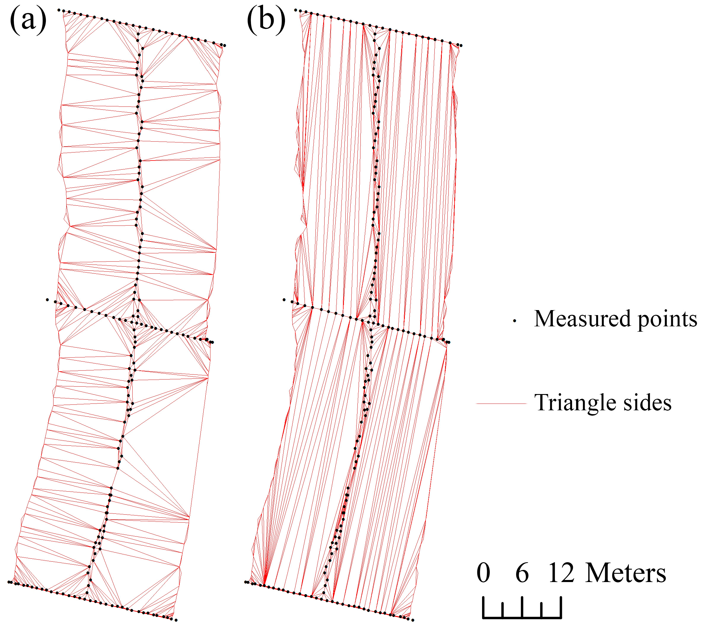
For large-scale measurements, the method with three cross-sections in addition to three longitudinal cross-sections seemed to be more accurate and show more detail than the other three methods. The results show that large-scale methods did not provide accurate results, similar to the findings of Jaballah et al., 2019 [2]. All methods had large areas with errors of more than 20 cm. Three cross-sections with one longitudinal section showed overestimation, while other methods had areas of both overestimation and underestimation, with a depth difference of around 20 cm. Thus, using these methods for the evaluation of the volumes of eroded or deposited sediments is not recommended. It must be noted that, if there is a long interval between cross-sections, it is recommended not to include a longitudinal profile in the calculations of DEMs when automatic Delaunay TIN is used as an interpolation method. These findings are in contrast to the hypothesis of Banjavcic and Schmidt 2018 [18], who indicated that longitudinal measurements can be combined to provide a better description of depth-averaged velocity throughout a river reach. Although the longitudinal section increased the accuracy around the measured path, it decreased the accuracy in areas near the banks. The reason is that the initial TIN was created based on the Delaunay method, which prevents the use of large, thin triangles for interpolation. As a result, the measured points in the banks were connected to points in the centerline for the interpolation of the unmeasured areas (Figure 15a). Therefore, it is also recommended to manually change the triangulations for methods with low measured point densities to increase the accuracy of the results. For the selected reach in this study, manually editing the created triangles changed the errors dramatically, especially for methods with low measured point densities (Figure 16b,d).
5. Conclusions
Different methods of measuring the bathymetry of water bodies were investigated in this study. The main goal of this study was to reduce the measurement time with the lowest reduction in accuracy.
One important aspect is to find an appropriate method for devices mounted on moving boats such as ADCPs. With these devices, very dense cross-sectional measurements provided more accurate results than any other measurement methods, but they are more time-consuming than zigzag measurements.
Overall, it is recommended to use regular grids, then cross-sectional measurements if no triangle editing is performed in the post-processing stages. Zigzag measurements had a very small percentage of error in central regions and most of the error was created in regions near the banks, on one hand. On the other hand, zigzag measurements reduced the workload to a greater extent than the other methods. The errors in the banks for the zigzag measurements could be reduced by manually editing the interpolation triangles.
The longitudinal measurement of the riverbed provided accurate information on bed changes in the center line, where the profile is passed; accounting for these points with wide cross-sectional measurements increased the overestimation error if the interpolated triangles were not manually edited.
Overall, dense point measurements and dense cross-sections provide more accurate results, but these methods are very time-consuming, while zigzag measurements require lower effort in addition to having high accuracy in the center of the channels. Only the banks had higher errors under zigzag measurements, which could be improved by modifying the interpolation algorithms manually. These findings can also be extended to mapping hydraulic parameters.
Author Contributions
Conceptualization, M.M. and M.R.; methodology, M.M.; software, M.M.; validation, M.M.; formal analysis, M.M.; investigation, M.M.; resources, M.M.; data curation, M.M. and M.R.; writing—original draft preparation, M.M.; writing—review and editing, M.M. and M.R.; visualization, M.M.; supervision, M.R.; project administration, M.R.; funding acquisition, M.R. All authors have read and agreed to the published version of the manuscript.
Funding
This research received no external funding.
Data Availability Statement
Data are available upon reasonable request from the corresponding author.
Acknowledgments
The authors would like to acknowledge the technicians from the Water Engineering Department of Shahid Bahonar University of Kerman, who provided support during measurements.
Conflicts of Interest
The authors declare no conflict of interest.
References
- Schäppi, B.; Perona, P.; Schneider, P.; Burlando, P. Integrating river cross section measurements with digital terrain models for improved flow modelling applications. Comput. Geosci. 2010, 36, 707–716. [Google Scholar] [CrossRef]
- Jaballah, M.; Camenen, B.; Paquier, A.; Jodeau, M. An optimized use of limited ground based topographic data for river applications. Int. J. Sediment Res. 2019, 34, 216–225. [Google Scholar] [CrossRef]
- Milan, D.J.; Hetherington, D.; Heritage, G.L. Application of a 3D laser scanner in the assessment of a proglacial fluvial sediment budget. Earth Surf. Process. Landf. 2007, 32, 1657–1674. [Google Scholar] [CrossRef]
- Rumsby, B.T.; Brasington, J.; Langham, J.A.; McLelland, S.J.; Middeton, R.; Rollinson, G. Monitoring and modelling particle and reach-scale morphological change in gravel-bed rivers: Applications and challenges. Geomorphology 2008, 93, 40–54. [Google Scholar] [CrossRef]
- Wang, J.; Shi, B.; Yuan, Q.; Zhao, E.; Bai, T.; Yang, S. Hydro-geomorphological regime of the lower Yellow river and delta in response to the water-sediment regulation scheme: Process, mechanism and implication. Catena 2022, 219, 106646. [Google Scholar] [CrossRef]
- Kummu, M.; Varis, O. Sediment-related impacts due to upstream reservoir trapping, the Lower Mekong River. Geomorphology 2007, 85, 275–293. [Google Scholar] [CrossRef]
- Bengora, D.; Khiari, L.; Gallichand, J.; Dechemi, N.; Gumiere, S. Optimizing the dataset size of a topo-bathymetric survey for Hammam Debagh Dam, Algeria. Int. J. Sediment Res. 2018, 33, 518–524. [Google Scholar] [CrossRef]
- Nikora, V.; Roy, A.G. Secondary flows in rivers: Theoretical framework, recent advances, and current challenges. In Gravel-Bed Rivers: Processes, Tools, Environments; Wiley: Chichester, UK, 2012; pp. 3–22. [Google Scholar]
- Charles, J.A. The engineering behavior of fill materials and its influence on the performance of embankment dams. Dams Reserv. 2009, 19, 21–33. [Google Scholar] [CrossRef]
- Brasington, J.; Langham, J.; Rumsby, B. Methodological sensitivity of morphometric estimates of coarse fluvial sediment transport. Geomorphology 2003, 53, 299–316. [Google Scholar] [CrossRef]
- Legleiter, C.J. Remote measurement of river morphology via fusion of LiDAR topography and spectrally based bathymetry. Earth Surf. Process. Landf. 2012, 37, 499–518. [Google Scholar] [CrossRef]
- Woodget, A.S.; Carbonneau, P.E.; Visser, F.; Maddock, I.P. Quantifying submerged fluvial topography using hyper spatial resolution UAS imagery and structure from motion photogrammetry. Earth Surf. Process. Landf. 2015, 40, 47–64. [Google Scholar] [CrossRef]
- Heritage, G.L.; Milan, D.J.; Large, A.R.G.; Fuller, I.C. Influence of survey strategy and interpolation model on DEM quality. Geomorphology 2009, 112, 334–344. [Google Scholar] [CrossRef]
- Carley, J.; Pasternack, G.B.; Wyrick, J.R.; Barker, J.R.; Bratovich, P.M.; Massa, D.A.; Reedy, G.D.; Johnson, T.R. Significant decadal channel change 58-67 years post-dam accounting for uncertainty in topographic change detection between contour maps and point cloud models. Geomorphology 2012, 179, 71–88. [Google Scholar] [CrossRef]
- Fuller, I.C.; Large, A.R.G.; Milan, D.J. Quantifying development and sediment transfer following chute cutoff in a wandering gravel-bed river. Geomorphology 2003, 54, 307–323. [Google Scholar] [CrossRef]
- Legleiter, C.J.; Kyriakidis, P.C. Spatial prediction of river channel topography by kriging. Earth Surf. Process. Landf. 2008, 33, 841–867. [Google Scholar] [CrossRef]
- Wheaton, J.M.; Brasington, J.; Darby, S.E.; Sear, D.A. Accounting for uncertainty in DEMs from repeat topographic surveys: Improved sediment budgets. Earth Surf. Process. Landf. 2010, 35, 136–156. [Google Scholar] [CrossRef]
- Banjavcic, S.D.; Schmidt, A.R. Spatial uncertainty in depth averaged velocity determined from stationary, transect, and longitudinal ADCP measurements. J. Hydraul. Eng. 2018, 144, 04018070. [Google Scholar] [CrossRef]
- Martirosyan, A.V.; Ilyushin, Y.V.; Afanaseva, O.V. Development of a distributed mathematical model and control system for reducing pollution risk in mineral water aquifer systems. Water 2022, 14, 151. [Google Scholar] [CrossRef]
- Ilyushin, Y.V.; Asadulagi, M.-A.M. Development of a Distributed Control System for the Hydrodynamic Processes of Aquifers, Taking into Account Stochastic Disturbing Factors. Water 2023, 15, 770. [Google Scholar] [CrossRef]
- Rennie, C.D.; Church, M. Mapping spatial distribution and uncertainty of water and sediment flux in a large gravel bed river reach using an acoustic Doppler current profiler. J. Geophys. Res. 2010, 115, F03035. [Google Scholar] [CrossRef]
- Milan, D.J. Terrestrial laser-scan derived topographic and roughness data for hydraulic modelling of gravel-bed rivers. In Laser Scanning for the Environmental Sciences; Heritage, G.L., Large, A.R.G., Eds.; Wiley-Blackwell: Chichester, UK, 2009; pp. 133–146. [Google Scholar]
- Fuller, I.C.; Large, A.R.G.; Heritage, G.L.; Milan, D.J.; Charlton, M.E. Derivation of reach-scale sediment transfers in the River Coquet, Northumberland, UK. In Fluvial Sedimentology VII, IAS Special Publication; Blum, M., Marriott, S., Leclair, S., Eds.; Wiley-Blackwell: Chichester, UK, 2005; Volume 35, pp. 61–74. [Google Scholar]
- Maleika, W.; Palczynski, M.; Frejlichowski, D. Interpolation methods and the accuracy of bathymetric seabed models based on multibeam echosounder data. In Intelligent Information and Database Systems; Pan, J.S., Chen, S.M., Nguyen, N.T., Eds.; ACIIDS 2012, Lecture Notes in Computer Science 7198; Springer: Berlin/Heidelberg, Germany, 2012; pp. 466–475. [Google Scholar]
- Hera, Á.; López-Pamo, E.; Santofimia, E.; Gallego, G.; Morales, R.; Durán–Valsero, J.J.; Murillo-Díaz, J.M. A case study of geometric modelling via 3-d point interpolation for the bathymetry of the Rabasa lakes (Alicante, Spain). In Mathematics of Planet Earth; Pardo-Igúzquiza, E., Guardïola-Albert, C., Heredia, J., Moreno-Merino, L., Duran, J., Vargas-Guzman, J., Eds.; Lecture Notes in Earth System Sciences; Springer: Berlin/Heidelberg, Germany, 2014; pp. 503–506. [Google Scholar]
- Bechler, A.; Romary, T.; Jeannée, N.; Desnoyers, Y. Geostatistical sampling optimization of contaminated facilities. Stoch. Environ. Res. Risk Assess. J. 2013, 27, 1967–1974. [Google Scholar] [CrossRef]
- Wang, J.; Yang, R.; Bai, Z. Spatial variability and sampling optimization of soil organic carbon and total nitrogen for minesoils of the Loess Plateau using geostatistics. Ecol. Eng. 2015, 82, 159–164. [Google Scholar] [CrossRef]
- Erdogan, S.A. comparison of interpolation methods for producing digital elevation models at the field scale. Earth Surf. Process. Landf. 2009, 34, 366–376. [Google Scholar] [CrossRef]
- Lane, S.N. The use of digital terrain modelling in the understanding of dynamic river systems. In Landform Monitoring, Modelling and Analysis; Lane, S.N., Richards, K.S., Chandler, J.H., Eds.; John Wiley and Son Ltd.: Chichester, UK, 1998; pp. 311–342. [Google Scholar]
- Gaeuman, D.; Jacobson, R.B. Aquatic Habitat Mapping with an Acoustic Doppler Current Profiler: Considerations for Data Quality; U.S. Geological Survey Open File Report; USGS: Reston, VA, USA, 2005; p. 1163. [Google Scholar]
- Dinehart, R.L.; Burau, J.R. Averaged indicators of secondary flow in repeated acoustic Doppler current profiler crossings of bends. Water Resour. Res. 2005, 41, W09405. [Google Scholar] [CrossRef]
- Parsons, D.R.; Best, J.L.; Lane, S.N.; Orfeo, O.; Hardy, R.J.; Kostaschuk, R. Form roughness and the absence of secondary flow in a large confluence-diffluence, Rio Parana, Argentina. Earth Surf. Process. Landf. 2007, 32, 155–162. [Google Scholar] [CrossRef]
- Jackson, P.R. Mississippi River ADCP Data; USGS: Reston, VA, USA, 2017. [Google Scholar]
- Williams, R.D.; Brasington, J.; Hicks, M.; Measures, R.; Rennie, C.D.; Vericat, D. Hydraulic validation of two-dimensional simulations of braided river flow with spatially continuous ADCP data. Water Resour. Res. 2013, 49, 5183–5205. [Google Scholar] [CrossRef]
- Flener, C.; Wang, Y.; Laamanen, L.; Kasvi, E.; Vesakoski, J.M.; Alho, P. Empirical modeling of spatial 3D flow characteristics using a remote-controlled ADCP system: Monitoring a spring flood. Water 2015, 7, 217–247. [Google Scholar] [CrossRef]
- Krüger, R.; Karrasch, P.; Bernard, L. Evaluating Spatial Data Acquisition and Interpolation Strategies for River Bathymetries. In Geospatial Technologies for All; Mansourian, A., Pilesjö, P., Harrie, L., van Lammeren, R., Eds.; AGILE 2018, Lecture Notes in Geoinformation and Cartography; Springer: Cham, Switzerland, 2018. [Google Scholar]
- Aggett, G.R.; Wilson, J.P. Creating and coupling a high-resolution DTM with a 1-D hydraulic model in a GIS for scenario-based assessment of avulsion hazard in a gravel bed river. Geomorphology 2009, 113, 21–34. [Google Scholar] [CrossRef]
- Andes, L.C.; Cox, A.L. Rectilinear inverse distance weighting methodology for bathymetric cross-section interpolation along the Mississippi River. J. Hydrol. Eng. 2017, 22, 04017014. [Google Scholar] [CrossRef]
- Jamieson, E.C.; Rennie, C.D.; Jacobson, R.B.; Townsend, R.D. 3-D flow and scour near a submerged wing dike: ADCP measurements on the Missouri River. Water Resour. Res. 2011, 47, W07544. [Google Scholar] [CrossRef]
- Puente, C.E.; Bras, R.L. Disjunctive kriging, universal kriging, or no kriging: Small sample results with simulated fields. Math. Geol. 1986, 18, 287–305. [Google Scholar] [CrossRef]
- Moore, I.D.; Grayson, R.B.; Ladson, A.R. Digital terrain modelling: A review of hydrological, geomorphological, and biological applications. Hydrol. Process. 1991, 5, 3–30. [Google Scholar] [CrossRef]
- Fuller, I.C.; Hutchinson, E. Sediment flux in a small gravel-bed stream: Response to channel remediation works. N. Z. Geogr. 2007, 63, 169–180. [Google Scholar] [CrossRef]
- Chaplot, V.; Darboux, F.; Bourennane, H.; Leguedois, S.; Silvera, N.; Phachomphon, K. Accuracy of interpolation techniques for the derivation of digital elevation models in relation to landform types and data density. Geomorphology 2006, 77, 126–141. [Google Scholar] [CrossRef]
- Yue, T.; Du, Z.; Song, D.; Gong, Y. A new method of surface modelling and its application to DEM construction. Geomorphology 2007, 91, 161–172. [Google Scholar] [CrossRef]
- Glenn, J.; Tonina, D.; Morehead, M.; Fiedler, F.; Benjankar, R. Effect of transect location, transect spacing and interpolation methods on river bathymetry accuracy. Earth Surf. Process. Landf. 2016, 41, 1185–1198. [Google Scholar] [CrossRef]
Figure 1.
Regular measurement grids with dimensions of 1 m2, 4 m2, 9 m2, 16 m2, and 25 m2 from left to right.
Figure 1.
Regular measurement grids with dimensions of 1 m2, 4 m2, 9 m2, 16 m2, and 25 m2 from left to right.

Figure 2.
(a) Cross-sectional measurements with a point interval of 1 m along the path for cross-sectional intervals of 1 m, 2 m, 3 m, 4 m, and 5 m; (b) longitudinal measurements with a point interval of 1 m along the longitudinal path and transverse intervals of 2 m, 3 m, 4 m, 5 m, and 6 m.
Figure 2.
(a) Cross-sectional measurements with a point interval of 1 m along the path for cross-sectional intervals of 1 m, 2 m, 3 m, 4 m, and 5 m; (b) longitudinal measurements with a point interval of 1 m along the longitudinal path and transverse intervals of 2 m, 3 m, 4 m, 5 m, and 6 m.

Figure 3.
Zigzag measurement methods with different side intervals of 2 m, 4 m, 6 m, 8 m, and 10 m. The bottom-right scheme is for half of the reach length’s zigzag movement.
Figure 3.
Zigzag measurement methods with different side intervals of 2 m, 4 m, 6 m, 8 m, and 10 m. The bottom-right scheme is for half of the reach length’s zigzag movement.

Figure 4.
Quick measurements where cross sections were measured with a very long interval in addition to one central and three longitudinal profiles.
Figure 4.
Quick measurements where cross sections were measured with a very long interval in addition to one central and three longitudinal profiles.

Figure 5.
Evaluating the accuracy of different interpolation methods for different point density measurements (a–d).
Figure 5.
Evaluating the accuracy of different interpolation methods for different point density measurements (a–d).

Figure 6.
DEMs extracted from regular gridded surveying methods.

Figure 7.
DEMs extracted from (a) cross-sectional and (b) longitudinal surveying methods.

Figure 8.
DEMs extracted from different zigzag surveying methods.

Figure 9.
DEMs extracted from different combinational surveying methods.

Figure 10.
The volumes of under/overestimation of the riverbed by different methods of surveying, in addition to measured point density and fieldwork (black line).
Figure 10.
The volumes of under/overestimation of the riverbed by different methods of surveying, in addition to measured point density and fieldwork (black line).

Figure 11.
Depths of under/overestimation of different regular gridded surveying methods.

Figure 12.
Depths of under/overestimation of (a) longitudinal and (b) cross-sectional surveying methods.
Figure 12.
Depths of under/overestimation of (a) longitudinal and (b) cross-sectional surveying methods.

Figure 13.
Depths of under/overestimation of different (a) zigzag and (b) combined surveying methods.
Figure 13.
Depths of under/overestimation of different (a) zigzag and (b) combined surveying methods.

Figure 14.
Real bed elevation of a cross section (black line) and the effects of the distance between two repeated measurement points on the overestimation volumes (orange and red zones).
Figure 14.
Real bed elevation of a cross section (black line) and the effects of the distance between two repeated measurement points on the overestimation volumes (orange and red zones).

Figure 15.
(a) The initial triangulations and (b) manual triangulations for interpolating unmeasured areas for the measurements with three cross sections and one longitudinal section.
Figure 15.
(a) The initial triangulations and (b) manual triangulations for interpolating unmeasured areas for the measurements with three cross sections and one longitudinal section.

Figure 16.
Depths of under/overestimation of the (a) initial triangulation for three cross sections and one longitudinal section, (b) manual triangulation for three cross sections and one longitudinal section, (c) initial triangulation for 5 m zigzag, and (d) manual triangulation for 5 m zigzag surveying methods.


Table 1.
Description of the selected reach.
| L 1 (m) | W 2 (m) | h 3 (m) | U 4 (m/s) | Q 5 (m3/s) | d50 6 (mm) |
|---|---|---|---|---|---|
| 90 | 24 | 0.3 | 0.8 | 5 | 30 |
Notes: 1 Length of the reach; 2 average width of the reach; 3 average water depth; 4 average flow velocity; 5 discharge during measurements; 6 median size of bed materials for which 50% are larger than it.
Disclaimer/Publisher’s Note: The statements, opinions and data contained in all publications are solely those of the individual author(s) and contributor(s) and not of MDPI and/or the editor(s). MDPI and/or the editor(s) disclaim responsibility for any injury to people or property resulting from any ideas, methods, instructions or products referred to in the content. |
© 2023 by the authors. Licensee MDPI, Basel, Switzerland. This article is an open access article distributed under the terms and conditions of the Creative Commons Attribution (CC BY) license (https://creativecommons.org/licenses/by/4.0/).
Share and Cite
MDPI and ACS Style
Maddahi, M.; Rahimpour, M. Effects of Spatial Data Acquisition on Determination of a Gravel-Bed River Geomorphology. Water 2023, 15, 1719. https://doi.org/10.3390/w15091719
AMA Style
Maddahi M, Rahimpour M. Effects of Spatial Data Acquisition on Determination of a Gravel-Bed River Geomorphology. Water. 2023; 15(9):1719. https://doi.org/10.3390/w15091719
Chicago/Turabian StyleMaddahi, Mohammadreza, and Majid Rahimpour. 2023. "Effects of Spatial Data Acquisition on Determination of a Gravel-Bed River Geomorphology" Water 15, no. 9: 1719. https://doi.org/10.3390/w15091719
Note that from the first issue of 2016, this journal uses article numbers instead of page numbers. See further details here.