

A Screening Procedure for Identifying Drought Hot-Spots in a Changing Climate

Department of Civil, Environmental and Mechanical Engineering, University of Trento, Via Mesiano 77, I-38123 Trento, Italy
*
Author to whom correspondence should be addressed.
Water 2023, 15(9), 1731; https://doi.org/10.3390/w15091731
Submission received: 16 March 2023
/
Revised: 21 April 2023
/
Accepted: 25 April 2023
/
Published: 29 April 2023
(This article belongs to the Special Issue Challenges of Hydrological Drought Monitoring and Prediction)
Abstract
:Droughts are complex natural phenomena with multifaceted impacts, and a thorough drought impact assessment should entail a suite of adequate modelling tools and also include observational data, thus hindering the feasibility of such studies at large scales. In this work we present a methodology that tackles this obstacle by narrowing down the study area to a smaller subset of potential drought hot-spots (i.e., areas where drought conditions are expected to be exacerbated, based on future climate projections). We achieve this by exploring a novel interpretation of a well-established meteorological drought index that we link to the hydrological drought status of a catchment by calibrating its use on the basis of streamflow observational data. We exemplify this methodology over 25 sub-catchments pertaining to the Adige catchment. At the regional level, our findings highlight how the response to meteorological drought in Alpine catchments is complex and influenced by both the hydrological properties of each catchment and the presence of water storage infrastructures. The proposed methodology provides an interpretation of the hydrologic behavior of the analyzed sub-catchments in line with other studies, suggesting that it can serve as a reliable tool for identifying potential drought hot-spots in large river basins.
1. Introduction
The Italian Alps are historically regarded as Europe’s water tower, hosting in their glaciers, snowfields, and aquifers the majority of freshwater feeding major European water streams such as the Danube, Rhine, Po, and Rhone rivers [1]. Despite not being traditionally threatened by persistent drought due to its continental climate and high altitude, the Alpine region has been declared at drought risk for more than a decade [2] as a consequence of the current trends of changing climate and of the reduction of its water resources [3,4], as well as of the projected increases in competing water uses that are to be expected in the future [5,6,7].
The projected trends in precipitation for the next century foresee a substantial decrease over the Alpine region, accompanied by a stronger reduction in the frequency and intensity of rainfall events during the summer season and a simultaneous increase in extreme events concentrated during cold seasons [8]. The average temperature in the Alpine region increased by about 2 °C during the 20th century, at a rate which is about two times higher than the Northern Hemisphere average [9]; moreover, an average warming of 0.25 °C per decade is expected over the Alps for the first half of the 21st century, a rate that is projected to increase to 0.36 °C per decade during the second half of the century [10]. A possible explanation for this faster-increasing trend is to be found in the snow-albedo feedback as indicated by the recent works of Pepin and Lundquist [11], Scherrer et al. [12], Notarnicola [13]. In this respect, the projected combination of meteorological changes toward a dryer, hotter, and more extreme climate threatens the onset of worsening drought conditions in the Alpine region [14].
Droughts, which can be defined as extended periods of time characterized by below-average water availability, can be further broken down into consequential events that usually take place in a chronological order: First, decreased rainfall causes the so-called meteorological drought. In combination with high temperatures, this results in increased evapotranspiration and decreased soil moisture availability, known as agricultural drought. Finally, the effect of anthropogenic stressors (e.g., industrial and household water usage, seasonal water storage, irrigation, etc.) on water reserves such as lakes and aquifers might result in decreased streamflow, often referred to as hydrological drought [15]. Notably, freshwater availability is crucial in several sectors related to the social–economical–ecological nexus of the Alpine communities and environment, such as agriculture [16,17], biodiversity [18], winter tourism [19], and hydropower generation [20,21,22]; in turn, this has led to increasing scientific and institutional interest in drought monitoring and prediction, often leading to the development of a variety of indexes, predictive tools, and early warning systems (see, e.g., [23,24,25], etc.).
Meteorological droughts over the Alps showed a shift towards prolonged events over the last two centuries [26] and are predicted to increase during the 21st century due to climate change [27], although it was suggested that the strength of a given drought signal strongly depends on the considered index [28] and that the use of different indexes might even lead to conflicting results [29]. Furthermore, droughts are complex phenomena, caused by a combination of events and pre-existing hydro-meteorological conditions, rendering the possibility to validate the use of any drought indexes or to set up warning systems based exclusively on observed data a very challenging task, especially in the case of large spatial domains [30]. A first attempt at compiling a systematic inventory of recorded drought events and climate evolution was recently made by an international consortium (ADO, ref. [31]).
Noticeably, the reliable identification of present and future drought conditions in the Alpine region carries several peculiarities that must be faced with adequate tools. First, Alpine catchments are characterized by complex orography: to adequately cope with this, the adopted climate models should be highly resolved in space and time and convective permitting (i.e., that explicitly accounts for variations in precipitation due to altitude) (see [32]), involving high computational costs. To the same end, detailed precipitation and evapotranspiration observational datasets should be made available in order to reliably validate or bias-correct the chosen climate models.
Managers and policymakers are often interested in hydrological and agricultural drought modelling, which must include a thorough assessment of the potential stress on a catchment’s water resources exerted by different and often competing water uses. In this context, predictive drought modeling should explicitly consider the relevant processes and characteristics of the domain [33] and should quantitatively assess the interactions occurring between the study area in its natural conditions and the main alteration due to anthropogenic water uses (see, e.g., [34,35]). Furthermore, it should be taken into account that different systems (e.g., agriculture, ecosystem, hydrology, etc.) respond to drought conditions at different timescales [36], which are in turn influenced by case-specific land use and resource management [37]. Considering the huge number of uncertainty factors revolving around drought prediction together with the related costs (e.g., computational demand, efforts for data collection, impact evaluation, etc.), it comes as no surprise that statistical indexes are the most widely used approach to investigate such complex phenomena. The Standardized Precipitation Index (ref. [38], SPI) and Standardized Precipitation Evapotranspiration Index (ref. [39], SPEI) are indeed the most widely used statistical indexes for large-scale drought assessment. Such indexes have been adopted in several regions to evaluate drought conditions during both historical (see, e.g., [40,41]) and future time periods (see, e.g., [14,27,42,43]). Notably, the mutual relationship between meteorological and hydrological drought indicators has catalyzed increasing attention in the last years (see, e.g., [44,45,46,47]), acknowledging the existence of multiple interplaying factors that should be considered in drought assessment.
To partially overcome the aforementioned challenges associated with a thorough drought assessment, we propose a reliable, yet parsimonious approach that is suitable for identifying potential drought hot-spots in the context of climate change, leveraging rainfall and streamflow observations for a reference historical period and climatic projections for the future period. The identification of the areas at drought risk by means of this preliminary screening will allow for a more focused investigation and efficient allocation of the available resources. Being parsimonious, the methodology is ideal for screening large domains before resorting to more detailed procedures and tools for the climatological, hydrological, and data collection analysis. We show an application of the developed methodology to the Adige catchment, whose sub-catchments can be considered representative of the hydro-climatological conditions observed in several Alpine watersheds.
This paper is organized as follows: in Section 2 and Section 3 we present the study area and the data used in our approach, respectively; Section 4 provides an overview of the adopted methodology. Section 5 showcases the results of our investigation, while in Section 6 we discuss our methodology and provide some considerations on its applicability in different contexts. Finally, in Section 7 we draw the final conclusions.
2. Study Area
This work focuses on the Adige catchment closed at the Vó Destro gauging station (identified by code IDRTN27 in Figure 1), with a total drainage area of 10,500 km2. The catchment is located in the eastern portion of the Italian Alps (see Figure 1) and is characterized by a complex topography, with mountainous areas reaching over 3800 m in altitude and downstream valleys around 200 m.a.s.l. Due to its morphology, precipitation is unevenly distributed within the catchment. Lower precipitation is typically observed in the highly elevated north-western part of the catchment (known as Val Venosta), averaging 600 mm/year, whereas an average precipitation of 1600 mm/year is observed at lower altitudes, especially in the southern part of the catchment; mean temperatures range from a minimum of −4 °C in January to a maximum of 14 °C in July, with a strong seasonal variability mainly related to the altitude [48,49]. Streamflows along the Adige’s main stem reach their minimum in winter when a large share of the precipitation is stored as snow; high flows are typically observed in early summer mainly due to snowmelt and then later in autumn due to cyclonic storms [49]; tributaries located in the north-western part of the catchment (which has the highest average altitude) exhibit a typically glacio-nival streamflow regime, with low flows in winter and high flows in summer due to ice- and snowmelt. Finally, the north-eastern headwaters show an intermediate behavior, defined as nivo-pluvial, where earlier peak flows occur in late spring and relatively high flows are observed in autumn [50]. The entire Adige catchment is strongly regulated by a number of reservoirs and diversion channels that exploit freshwaters for hydropower production [51,52,53], exerting a strong control on downstream flow regimes. Table 1 summarizes some properties of the sub-catchments analyzed in the present work: the cumulative effective storage () present within each sub-catchment, the average streamflow () for each sub-catchment, and the recharge coefficient , computed as the ratio between the former and the latter [51], which provides an estimate of the degree of regulation of each sub-catchment. Finally, the temporal coverage of monthly average streamflow time series is provided for each sub-catchment (, which computation will be further detailed in the ensuing Section 3.3). The heterogeneous hydrological response to precipitation of the streams that are present within the Adige catchment is expected to increase as a consequence of the projected effects of climate change, thus making the Adige catchment a very interesting case for showcasing the proposed drought hot-spot screening methodology.
3. Data
Our proposed methodology takes advantage of the information provided by the spatially-distributed observational data of precipitation and air temperature to compute a meteorological drought index, which is then correlated to a hydrological drought index computed on the basis of historical streamflow observations collected during the same period (see Section 3.1). Finally, the meteorological drought index is computed for the future time window on the basis of available climatological model data (presented in Section 3.2).
3.1. Observational Data
Monthly precipitation and evapotranspiration time series for the catchments under investigation were computed on the basis of daily information provided by the ADIGE meteorological dataset [49]. The dataset consists of daily observations at 244 and 350 gauging stations for precipitation and air temperature, respectively, that have been distributed on a km grid using the Ordinary Kriging with External Drift (OKED) method, adopting elevation as the secondary variable [54]. Starting from the minimum, maximum, and mean daily air temperature present in the dataset, the daily potential evapotranspiration (PET) was computed, according to the Hargreaves–Samani approach [55] for each grid cell. We note that the ADIGE dataset was found to be the most reliable dataset for reproducing the observed streamflows in the Adige catchment [48]. The ADIGE dataset is available over the 1925–2013 time window with no gaps [49].
Daily streamflow observations at 25 stream gauging stations evenly spread within the Adige river basin (whose locations are shown in Figure 1) were provided by the Hydrological Offices of Trento (http://www.floods.it/public/, accessed on 21 February 2022) and Bolzano (http://www.provincia.bz.it/hydro/, accessed on 21 February 2022). The available measurements cover the 1956–2013 time window at a daily scale, with few gaps. The 25 stream-gauging stations identify the outlet of the sub-catchments, some of which are nested, which were considered in the present work to exemplify our proposed methodology.
3.2. Climate Model Data
The climate model data were retrieved from the EURO-CORDEX programme (COordinated Regional Downscaling EXperiment [56]), which provides future climate predictions over the European domain. In order to reduce the overall computational burden of our proposed methodology, we followed the selection procedure proposed by Vrzel et al. [57], who identified, by means of a clustering analysis, 3 climate model combinations (as provided by the selection of a driving Global Circulation Model, GCM, with a nested Regional Climate Model, RCM) which, among all, ensured the largest climatological variability over several analyzed catchments, including that of the Adige: the so-identified GCM–RCM combinations are synthesized in Table 2. In particular, we considered GCM–RCM combinations at a spatial resolution of about 12 km (EUR-11 ensemble). Note that the same 3 GCM–RCM combinations were adopted in a recent work by Majone et al. [58] that analyzed the impact of climate change on high streamflow extremes in the same study region. The adoption of this sub-selection serves the dual purpose of reducing the overall computational burden and of ensuring that the resulting outcome will entail the widest variety of scenarios, thus making the identification of future drought hot-spots less computationally expensive, yet accurate and reliable. Furthermore, in the analysis we only considered the RCP4.5 emission scenario, adopting the 1981–2010 time window as the reference period and the 2041–2070 time window as the future period. These datasets contain records of the daily precipitation and minimum, mean, and maximum temperature; similarly to what was performed for the observational data, the corresponding PET time series were computed according to Hargreaves and Samani [55].
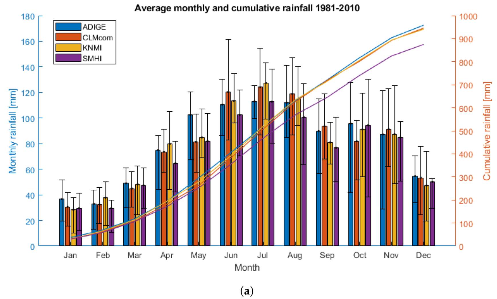
Figure 2 compares the monthly average and cumulative precipitation (Figure 2a) and monthly average temperature (Figure 2b) of the ADIGE dataset with those of the CORDEX models, which were spatially averaged over the entire catchment for the purpose of this comparison. The average precipitation in the ADIGE dataset is slightly higher than that of the CORDEX datasets in the first six months of the year, with the largest discrepancy observed in May (20 mm/month difference); in the second part of the year, the CLMcom and KNMI datasets provide slightly larger precipitation values than ADIGE, compensating for the first part of the year and resulting in similar cumulative yearly precipitation. On the other hand, SMHI slightly underestimates the precipitation and this is reflected in the annual cumulative value. The inter-annual variability of the models is similar, as captured by the similar inter-quartile range (IQR) bars depicted in Figure 2a and synthesized in Table 3. Concerning temperature, the CORDEX models exhibit slightly colder temperatures from September to March, resulting in an average bias of about 0.5 °C over the entire year. On the other hand, the monthly IQR values are comparable for all months, with an annual average in the range between 2.16 °C and 2.21 °C (see Table 4), thus supporting the conclusion that the four datasets are in substantial agreement as far as temperature is concerned. Finally, the R-squared correlation coefficient between the long-term monthly averages of ADIGE (i.e., 12 values of the barplot) and those of the CORDEX models was computed for both precipitation and temperature. These values (displayed at the bottom of Table 3 and Table 4) are very close to 1 in all cases, further supporting our conclusion about the overall similarity between the observed data and the chosen climate models over the Adige catchment in the reference period 1981–2010.
3.3. Preliminary Data Elaborations
Our methodology relies on the application of monthly indexes for each investigated sub-catchment. The sub-catchments are uniquely identified by a streamflow-gauging station at their closing point and are represented in Figure 1. Therefore, all data underwent preliminary processing in order to suit our analysis. The streamflow data at the gauging stations (available at a daily time scale) were considered as representative of their entire sub-catchment: in this case, the data were only averaged at the monthly scale, producing a time series of the average monthly streamflow for each sub-catchment. In particular, we retained only months in which 90% or more of the daily measurements were present (i.e., 27 or more days), while the other months were considered as missing values. The resulting percentage of time coverage associated with the monthly streamflow time series is summarized in Table 1.
The meteorological data provided by the ADIGE dataset were available at a daily time scale and on a km grid; therefore, they were first spatially aggregated at the sub-catchment level and subsequently at the monthly time scale. Spatial aggregation was performed considering the nested structure of the sub-catchments; therefore, all the upstream contributing sub-catchments were considered when computing the input time series for the downstream ones. The daily precipitation (P) values were averaged on all grid cells pertaining to each sub-catchment (spatial aggregation) and then cumulated for each month (temporal aggregation), yielding a monthly time series of precipitation for each catchment. Likewise, monthly time series of potential evapotranspiration (PET) were obtained starting from the daily PET data.
A similar procedure was carried out for obtaining monthly time series of P and PET starting from the daily data of the CORDEX datasets. In particular, the CORDEX data were resampled using the nearest-neighbor method to the ADIGE grid (1 km spacing) without performing an additional downscaling procedure.
4. Methodology
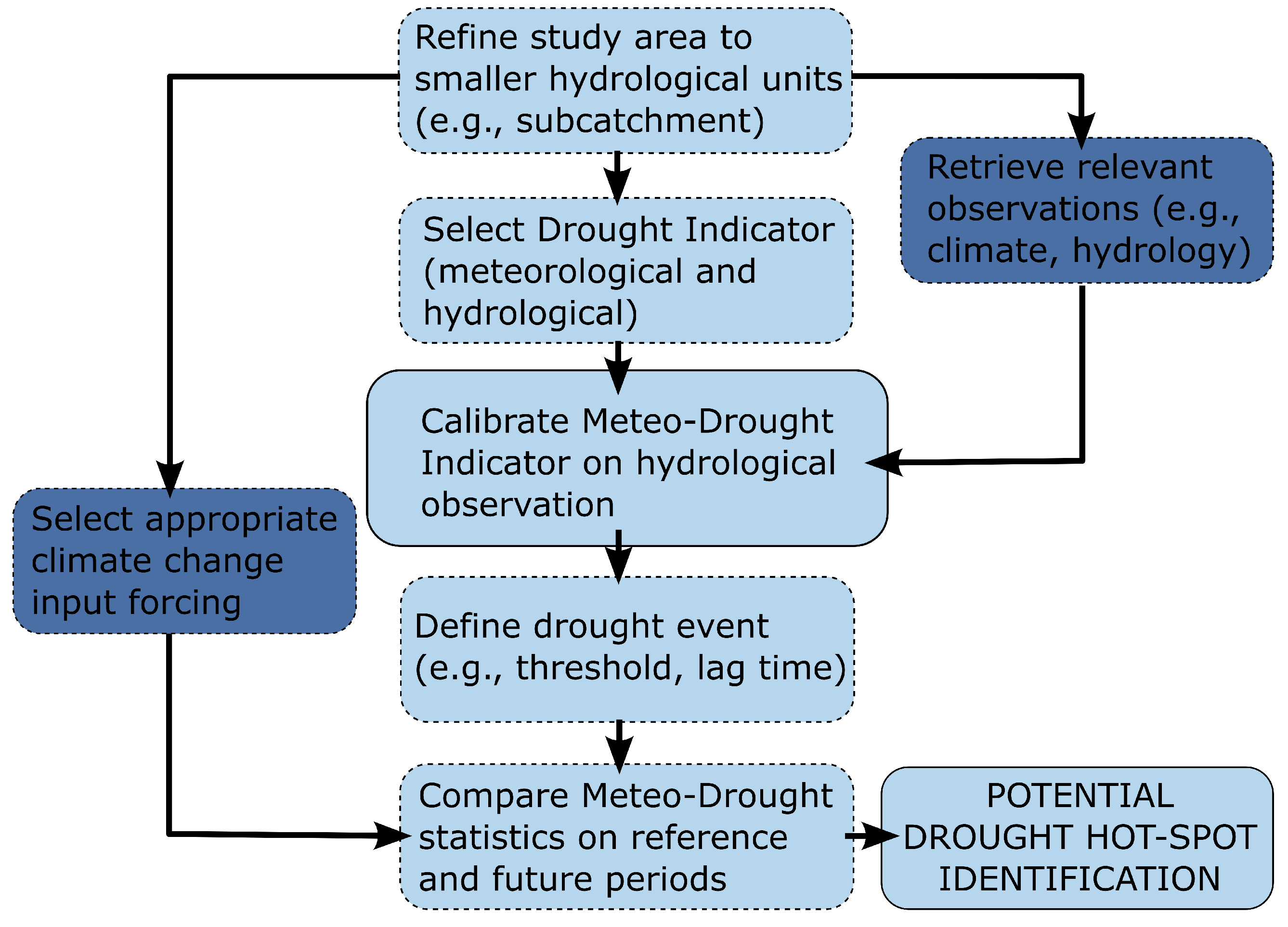
The framework adopted in our analysis is applied at the sub-catchment scale. First, the data are aggregated at the monthly time scale in each sub-catchment, as detailed in Section 3.3. The meteorological and hydrological drought indexes are then computed as detailed in Section 4.1 and Section 4.2, respectively. Subsequently, the meteorological drought index is associated with the hydrological response of each sub-catchment (i.e., streamflow time series), as detailed in Section 4.3. The meteorological drought index is then computed at each sub-catchment for the reference and future period. After defining proper thresholds for the identification of drought events, the variation in meteorological drought statistics between the future and reference periods is computed and adopted for hydrological drought hot-spot identification (as detailed in Section 4.5).
Details about the methodology are provided in the ensuing subsections whilst a graphical overview is depicted in Figure 3.
4.1. Meteorological Drought Index
The meteorological drought index adopted in this work is the Standardized Precipitation Evapotranspiration Index (SPEI) developed by Vicente-Serrano et al. [39]. The index is conceived as an extension of the widely applied Standardized Precipitation Index (SPI, ref. [38]): in SPEI, the input variable is provided by the normalized cumulative water deficit (D) as defined in Equation (1) in place of the normalized time series of cumulative precipitation used in the SPI. The SPEI is therefore designed to take into account both precipitation and potential evapotranspiration in determining the droughts and, contrary to SPI, it is able to capture the non-negligible impact of increased temperatures on the water budget.
In Equation (1), , and represent the deficit, precipitation, and potential evapotranspiration values during month i, respectively. Following the same procedure typically adopted for the SPI the calculated values are then aggregated over different timescales, :
where the summation indicates that at every i-th month, the preceding months (including the current one) are included in the computation of the aggregated water deficit. Depending on the target application, the timescales vary typically between 1 and 24 months. As an example, if the considered timescale is 3 months, the input value for January will consider the cumulative monthly water deficit of November, December, and January itself.
Standardization (i.e., normalization) of the water deficit variable (for a given timescale) is then performed independently for each month of the year by fitting the monthly deficit time series to a parametric cumulative distribution function (CDF) from which the non-exceeding probabilities are then transformed into a standard normal distribution (with mean and standard deviation ). This last transformation makes the SPEI easily interpretable, as its values represent the difference (in terms of multiples of standard deviations) between the current month and a reference value. The standardization procedure of the deficit values aggregated over a generic timescale () and the derivation of the corresponding SPEI index is exemplified in Figure 4. Several studies suggest the use of a log-logistic distribution [39] for fitting the water deficit time series, although a recent contribution suggests the generalized extreme values (GEV) distribution when referring to applications in Europe [59]. In this work we tested both distribution families with the Kolmogorov–Smirnov (KS) test and by computing the Akaike information criterion (AIC) to assess the most appropriate distribution for fitting the monthly water deficit time series. The results show that both distributions were not rejected from the KS test at a significance level of = 0.05 and that the log-logistic distribution presented the lowest average KS and AIC statistics (across all months and sub-catchments). In particular, for the monthly water deficit time series the KS average is 0.103 for GEV and 0.07 for log-logistic and the AIC average is 588.0 for GEV and 587.1 for log-logistic. Although the differences between GEV and log-logistic are small, the presented results justify the adoption of the latter as the distribution to adopt in our work. The parameters for each distribution were inferred using maximum likelihood estimation (MLE).
The interpretation of the SPEI time series depicted in Figure 4b attributes wetter-than-average conditions to SPEI values above the chosen threshold of 0 (highly positive values representing an extremely wetter month compared to the reference distribution for that month), whereas negative SPEI values represent dryer-than-average months.
4.2. Hydrological Drought Index
In this work, we also evaluated hydrological drought conditions of the investigated sub-catchment by computing the Standardized Streamflow Index (SSFI) [60,61]. Similarly to the SPEI, SSFI is also computed at the monthly time scale. The monthly streamflow time series were computed by averaging the observed daily streamflow time series available at the different gauging stations, as detailed in Section 3.3; standardization was then performed following the same procedure described for SPEI in Section 4.1. Furthermore, in this case, both log-logistic and GEV distributions were used as a fitting CDF for each month, with the former providing slightly better performances among all sub-catchments and months of the year. In particular, the KS average is 0.146 for GEV and 0.106 for log-logistic and the AIC average is 286.8 for GEV and 286.3 for log-logistic. Validation of the inference procedures was performed by means of the successful application of the Kolmogorov–Smirnov and Pearson tests. The SSFI time series were therefore computed considering a 1-month timescale, fitting a log-logistic distribution with MLE to each month’s average flows. The interpretation of the SSFI is similar to that of the SPEI, as positive values indicate higher-than-average streamflows, and vice versa.
4.3. Characteristic Timescale
For the purposes of our work, we introduce and adopt the concept of the characteristic timescale of a catchment. Indeed, meteorological drought indexes such as SPEI can be computed at any timescale; hence, their interpretation can vary widely (see, e.g., [23,39]). Our objective here is to link meteorological droughts to the hydrological drought conditions of a sub-catchment. In order to do so, we computed the SPEI at all timescales ranging between 1 and 12 months and the SSFI at the 1-month timescale; then, we selected as the characteristic timescale for a given sub-catchment the aggregation time for the SPEI leading to the highest linear correlation with the SSFI (computed with the Spearman rank correlation test [62]). This allows us to identify in a simplified way the hydrological response time of the sub-catchments, or, in other words, to estimate the average delay between the occurrence of the meteorological drought and reduced in-stream freshwater availability (i.e., hydrological drought).
SPEI was computed over the 1956–2013 time window based on precipitation and evapotranspiration data retrieved from the ADIGE dataset (cfr. Section 3.1), which was shown recently to provide the highest accuracy in reproducing the observed streamflow time series at selected gauging stations in the Adige river basin [48]. Similarly to the SPEI, SSFI was also computed over the 1956–2013 time window, based on monthly streamflow time series pertaining to each gauging station.
4.4. Identification and Definition of Drought Events
Once the characteristic timescale has been identified for each sub-catchment, drought events can be determined based on the monthly time series of SPEI values. The procedure is exemplified in Figure 4b. A drought event is considered to start whenever the SPEI value falls below a certain threshold and to end whenever the SPEI value goes back above it: the duration of a drought event is hence defined as the number of consecutive months during which the SPEI remains under the drought threshold. The intensity of the drought is the value of SPEI in a single month, while the severity of a drought event is the sum of the drought intensities within the duration of the event. The identification of the drought threshold is in principle arbitrary and can vary depending on the area under investigation and on the goals of the analysis, though most applications adopt values of 0 or −1. In this study we adopt 0 as the drought threshold value. Finally, the average frequency of drought events within a time window can be evaluated by computing the ratio between the total number of identified drought events and the period duration expressed in years.
4.5. Identification of Future Drought Hot-Spots
The screening for potential future drought hot-spots is performed by analyzing the variation of meteorological drought characteristics between the future (2041–2070) and reference (1981–2010) conditions. First, the median severity of drought events in both the reference and future time windows was computed, and then the two values were compared by computing their ratio, according to Equation (3):
where and represent the median of the severity values associated with drought events in the reference and future time windows, respectively. For the calculation of this index, the median severity was preferred over the mean: the drought event distribution indeed tends to be skewed towards extreme values; hence, the adoption of the median is preferable, as also suggested by other work on related topics (see, e.g., Barker et al. [63]).
Second, the number of dry months (i.e., months with SPEI lower than 0) in both the reference and future time windows was computed. Here, the comparison is shown in terms of percent variation over the whole period, computed according to Equation (4):
where and represent the number of months with SPEI values under the chosen threshold of 0 in the reference and future time windows, respectively, and 360 represents the number of months in each time window. Indeed, the severity and dry months are often used by local administrations and policymakers for drawing drought-response strategies. In this work, the identification of future drought hot-spots is indeed associated with the interpretation of the aforementioned indicators.
To this end, the characteristic timescales that have been identified for each sub-catchment using observational data (following the procedure described in Section 4.3) are here adopted for computing the SPEI index using the projections provided by the CORDEX datasets. The underlying hypothesis is that the hydrological response time to the meteorological droughts that was identified based on the observational datasets remains unchanged when applied to the future time window. This assumption is justified by the similarity between the observations and the climate model data in the reference period, as discussed in Section 3.2.
5. Results
5.1. Characteristic Timescale for Each Catchment
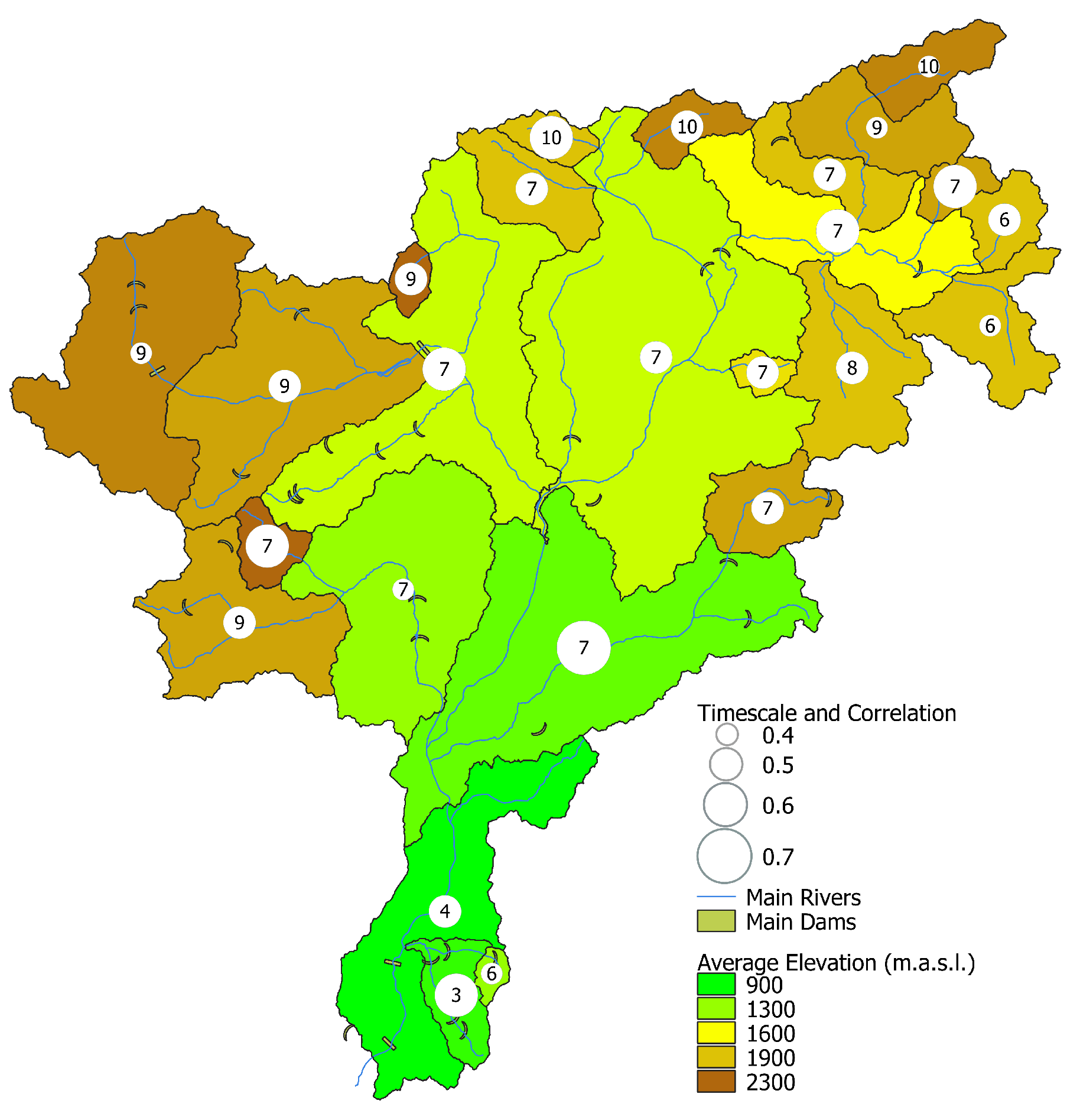
The characteristic timescales for each of the 25 sub-catchments investigated in this study were computed following the methodology described in Section 4.3: their values are summarized in Table 5 and visually presented in Figure 5. The timescales range between 6 and 10 months, with Spearman’s rank correlation scores ranging between 0.395 and 0.722. The correlation between SPEI and SSFI is statistically significant in all sub-catchments (p-values always lower than at a confidence level of 95%.
The results depicted in Figure 5 highlight that SPEI computed with a timescale of 7–9 months (here defined as long timescales) correlates better with SSFI in highly elevated sub-catchments, whereas the timescale of the highest correlation decreases moving towards downstream sub-catchments. However, visual inspection of Figure 5 also reveals some deviations in the spatial pattern followed by characteristic timescales and that some sub-catchments present relatively lower correlations (). We attribute this to two concurring, independent causes: first, the availability of observed streamflow time series, which can cover a limited timespan in some gauging stations, thus affecting the reliability of the rank-correlation computation; second, a stream-gauging station located immediately downstream of large anthropogenic water withdrawal or restitution infrastructure will inevitably record streamflow values that may be not representative of the natural hydrological response of a catchment.
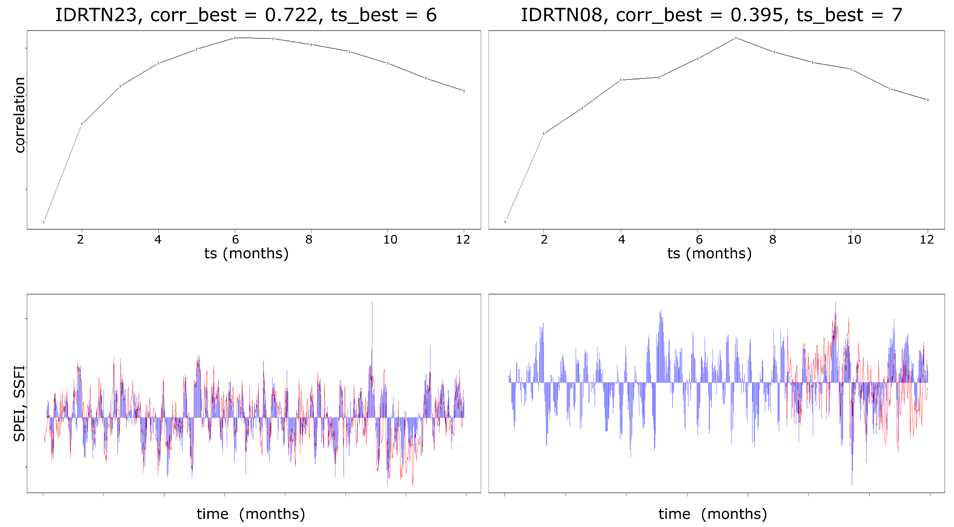
The correlation plots for the two sub-catchments presenting the highest (station IDRTN23) and lowest (station IDRTN27) Spearman’s rank correlation between SPEI and SSFI are displayed as an example in Figure 6. It is worth noting that for the IDRTN23 station the correlation exhibits a regular dependency with respect to changing timescales, benefiting from the availability of a long streamflow observation record. On the other hand, for the IDRTN27 station the correlation plot shows an irregular pattern, which can be attributed to the limited streamflow record (see the lower right inset of Figure 6). Furthermore, considering the temporal coverage of monthly time series and the recharge coefficient summarized in Table 1, it can be observed that low correlation values are often associated with a high degree of regulation (e.g., 05950PG, 19850PG, IDRTN08, IDRTN17, IDRTN21, and IDRTN27) or with reduced data availability (e.g., 43350PG, 51450PG, 57150PG, IDRTN17, IDRTN21, and IDRTN27). Finally, it should be noted that these two causes are most likely concurrent, with the former possibly influencing the latter in some cases.
5.2. Drought Hot-Spots
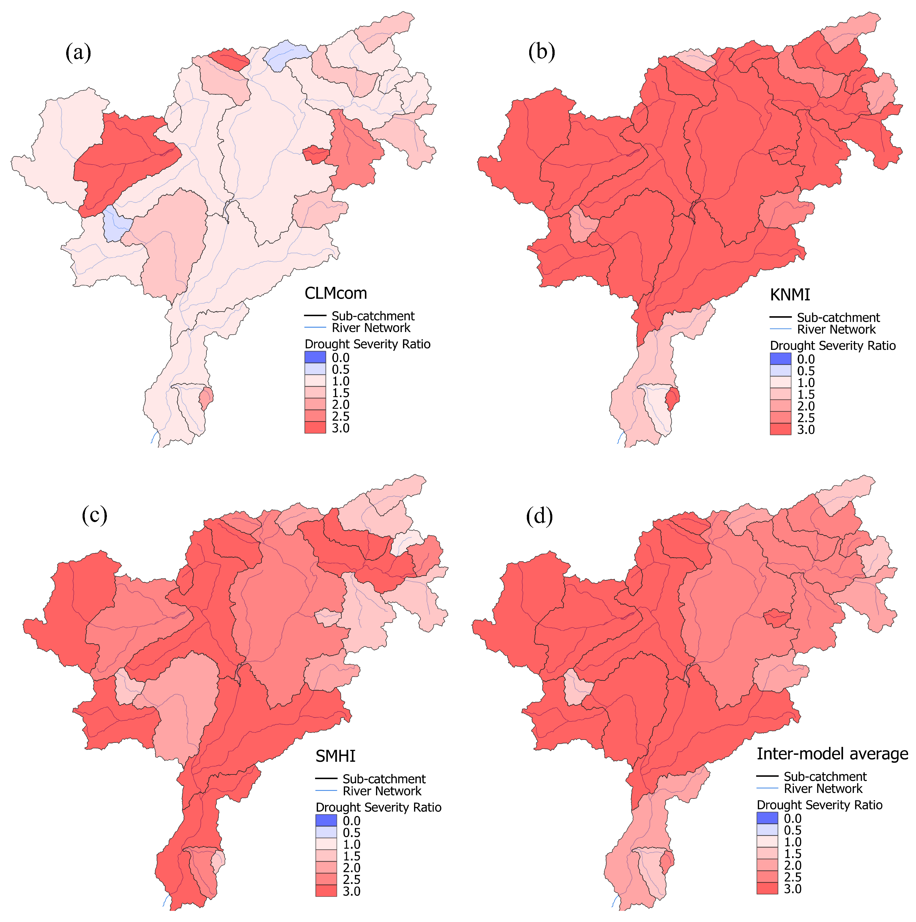
The characteristic timescales identified for each sub-catchment (see Table 5) were then employed to compute SPEI time series for each climate model simulation in the reference (1981–2010) and future (2041–2070) time windows. Based on these time series, the evolution of drought conditions was analyzed with reference to the drought severity and frequency indexes defined in Section 4.5.
The resulting values of the drought severity index for each climate model are displayed in Figure 7a–c, whereas panel (d) shows the inter-model average values. Moving from the reference time window to the future one, CLMcom projects the lowest increase in the average drought severity (, computed by averaging all the sub-catchments), with some sub-catchments facing a slight decrease (i.e., < 1, shaded in blue in Figure 7a); conversely, KNMI projects a widespread strong increase in drought severity in almost all of the considered sub-catchments () with respect to the reference time window. Finally, SMHI projects a larger-severity increase along Adige’s main stem, located in the central and north-western part of the river basin, whilst moderate increases of severity are observed in the upstream sub-catchments (). The inter-model average highlights that the north-western sub-catchments are more likely to face drought severity increases, according to all climate models.
As far as drought frequency is concerned, the results for the percentage variation in the total number of dry months are presented in Table 6. It can be observed that CLMcom shows a relatively large increase in the number of dry months (13% on average among all sub-catchments). KNMI projects the largest increase (17% average overall), whereas the SMHI projection concerning this index is the lowest overall (4%). Nevertheless, the inter-model average shows that an increase in dry months of 6–14% is to be expected among all sub-catchments.
6. Discussion
The main goal of this work is to provide a simple screening procedure to gauge potential threats to freshwater supplies posed by climate change. This is in line with the concept explored by Nayak et al. [64], with the difference that we do not rely on the use of a hydrological model to further reduce the complexity of the methodology and its inherent uncertainty. Indeed, relying on the use of a hydrological model to perform a thorough drought prediction involves the acquisition of reliable supporting information (e.g., land use, stressors to the water budget, etc.) and performing the simulation at a scale that can reliably simulate land-surface characteristics and small-scale processes in the atmosphere such as convection. As a consequence, the use of spatially-distributed hydrological models over large domains is often unfeasible. For this reason, our proposed framework exploits the information contained in measured streamflow time series to gauge the effects of meteorological forcing on the water budget [65] and allows us to calibrate the use of the SPEI for anticipating potential drought hot-spots based solely on meteorological projections provided by climate models.
6.1. Characteristic Timescales
The correlation analysis between SPEI and SSFI highlighted the timescale (at which SPEI is computed) that produces the highest correlation between the two indexes, termed the characteristic timescale of each sub-catchment. Noticeably, the results highlighted a dependency between the characteristic timescales and the average altitude of their respective sub-catchment. In particular, larger characteristic timescales (9–10 months) are observed in the high-elevation headwater sub-catchments, intermediate values (7–8 months) are found for the central and north-eastern part of the catchment, while the lowest characteristic timescales were found in the southern part of the catchment (3–7 months). Indeed, larger timescales are typically associated with a delayed hydrological response of glacier- and snow-dominated catchments (Eder et al. [66], Brauchli et al. [67]), whereas a shorter hydrological response to precipitation is more common in rainfall-dominated catchments (Soulsby et al. [68]). The spatial variability of the characteristic timescales among the sub-catchments resulting from our analysis is indeed in strong agreement with the findings of Larsen et al. [50], who categorized the hydrological regime of several reaches within the Adige catchment. Furthermore, López-Moreno et al. [69] highlighted that timescales of 6–10 months are characteristic of strongly regulated catchments, which is the case for the majority of the sub-catchments located in the northern part of the Adige basin as well as some side valleys in the southern part, as can be observed in Figure 5.
A similar practice of correlating SPEI with SSI (Standardized Streamflow Index, developed by Vicente-Serrano et al. [61], which shares many similarities with SSFI adopted in this work) was explored by Vicente-Serrano et al. [44] in the Iberian Peninsula. These authors also concluded that an informed use of the timescale parameter can explain the lag time between meteorological drought and the hydrological response and that the response time depends on the size and degree of regulation of a catchment, with large downstream catchments showing highest-correlating timescales at around 6 months. This latter result is indeed in strong agreement with our findings. The study of Wu et al. [46] also found that a non-linear relationship exists in the response time of hydrological drought to meteorological drought, highlighting that relevant dam operations caused a reduction in the hydrological drought severity and duration compared to the pre-existing natural conditions, although the delay time between meteorological and hydrological drought decreased significantly, similarly to what was found by Lorenzo-Lacruz et al. [45]. In the same study by Wu et al. [46], another interesting finding is the introduction of the propagation time concept (i.e., the lag time between the start of meteorological drought and the beginning of the related hydrological drought event). Such a concept is indeed similar to our concept of the characteristic time scale, though the propagation time is related to drought events obtained with a fixed accumulation time.
SPEI is commonly computed referring to canonical timescales (ranging from 1 to 12 months or above) and its values are linked to different types of hydrological response [39]. On the other hand, the concept of characteristic timescale adopted herein represents a shift in this paradigm, where the use of a meteorological drought index is calibrated against the observed response of a catchment (i.e., streamflow time series). The use of characteristic timescales in the computation of SPEI provides a simplified, yet reliable link between meteorological droughts and freshwater availability within each sub-catchment, indirectly accounting for all its related stressors. Despite our encouraging results, the interplay between rainfall and all of the natural and anthropogenic factors that underlie the hydrological response of a catchment is very complex and indeed calls for further investigation.
6.2. Drought Hot-Spots
Drought hot-spot identification was based on the comparison of aggregated drought severity and frequency indexes between the future and reference time windows. The projected variation in the drought severity ratio varies considerably among the climate models, each one presenting different spatial distribution and magnitude of the index. This result is indeed expected as the choice of the climate models we performed (see Vrzel et al. [57]) was aimed at preserving the maximum variability of the projections for the investigated case study. Indeed, mid-future (i.e., 2041–2070) precipitation anomalies over the Greater Alpine region vary considerably among all CORDEX models, as was also shown by Spinoni et al. [43]. In this sense, averaging the predictions of more climate models can provide further insight as to which areas can be confidently expected to become a drought hot-spot.
All climate model simulations project an increase in the number of dry months during the 2041–2070 time window compared to the reference period. The increase is evenly spread among all sub-catchments (see Table 6), and minor differences exist between the models, with KNMI projecting the largest increases and SMHI projecting the smallest. Linking this result with the projected large increases in severity (which is, de facto, the product of drought duration and its average intensity) leads to the conclusion that future dry spells might be more extreme while not necessarily more frequent. This result is in agreement with other studies conducted in the Italian Alpine region, which projected prolonged dry periods in the mid-future under RCP 4.5 emission scenario [14,43]. The authors attributed these results to widespread temperature increase and, to a minor extent, to the expected decrease in summer precipitation. It can also be noted that the dry-month variation projected by CLMcom come in slight opposition to what could be expected judging from Figure 7. Indeed, despite the projected severity only showing minor increases, the projected drought conditions will affect longer periods in the future.
We, therefore, argue that the joint evaluation of multiple drought event characteristics (i.e., drought severity and duration) is mandatory for a reliable prediction of future drought scenarios.
6.3. Strengths and Limitations of the Methodology
Drought prediction is a challenging task that requires complex modeling techniques and the availability of accurate input datasets. In this perspective, large-scale drought assessment often results in prohibitive computational demands. The proposed methodology aims to identify future drought hot-spots in a fast yet reliable manner, linking the interpretation of the SPEI index to the physical characteristics of each identified catchment by correlating it with observational streamflow and meteorological data. It is evident that the inherent drawback of such an approach is its reliance on high-quality data to ensure an accurate identification of the characteristic timescale. Indeed, we identified two pitfalls of our methodology when referring to stream-gauging stations in which streamflow time series are too short (Figure 6) and stations that are located close to significant alterations of the water budget (e.g., hydropower or agricultural water diversions, see, e.g., stations 05950PG, IDRTN08, and IDRTN17 in Figure 1). This can either lead to low correlation values or to less meaningful characteristic timescales (Table 5). Furthermore, it should also be noted that modifications to the storage capacity of the catchments (such as, e.g., variation in the effective storage capacities of hydropower reservoirs, changes in their operating policies or aquifer recharge management activities) could affect the characteristic response time of a catchment over a long time span. In this perspective, the hypothesis that the hydrological response time to the meteorological droughts remains constant in time might be substantial. On the other hand, water management in small storage reservoirs, as is the case for most systems present in the Adige, entails daily or weekly time scales, which are lower than the monthly time scales adopted in our framework and are therefore not affected by this kind of operation. Finally, we remark that our methodology should be considered a preliminary screening step of a more detailed drought assessment over large-scale watersheds, which typically require a wealth of information [51] and involve high computational effort [52] to set up a thorough hydrological modeling framework.
The framework presented in this paper aims to showcase the potentiality of a rapid screening procedure, although further research should be devoted to the identification of the most representative drought indexes, drought event definitions (threshold, lag-time, etc.), and statistical analyses aimed at the identification of drought hot-spots in order to generalize the presented framework. The selection is also strictly dependent on the area of investigation and on the personal decision of the modeler, and therefore, we decided to rely upon widely adopted drought indexes and definitions for the purposes of this work. Similar considerations might be drawn for the optimal selection of climate change scenarios and their related bias-adjustment techniques, the identification of which is, however, beyond the objectives of the present contribution.
7. Conclusions
In this work we propose a framework to quickly and reliably determine potential future drought hot-spots. The methodology is based on a novel interpretation of the SPEI index that is linked to the hydrological response of a catchment. This is achieved by correlating SPEI computed at several timescales (1 to 12 months) with the hydrological drought index SSFI: the timescale producing the highest correlation between the SPEI and SSFI monthly series is herein defined as the characteristic timescale of the catchment. To exemplify our approach we selected a well-instrumented watershed in the Italian Alpine region, the Adige river basin. The study area was subdivided into 25 sub-catchments and characteristic timescales were computed for each of them based on available meteorological and streamflow observations in the 1956–2013 time window. The characteristic timescales were then used to compute SPEI time series over a reference (1981–2010) and future (2041–2070) time window for three different climate model simulations under the RCP 4.5 emission scenario. The drought event statistics in these two periods and their inter-model average were then compared, highlighting which sub-catchments are more likely to face worsening drought conditions in the context of climate change.
This study also provides interesting insights at the regional scale. The evolution of drought statistics in the study area predicts widespread drying trends with variable intensities, which is in accordance with the findings of similar investigations. The spatial distribution of the resulting characteristic timescales exhibits a complex, yet clear dependence on the catchments’ hydrological regimes and the degree of streamflow regulation (i.e., reservoir storage) of each catchment. The spatial variability of characteristic timescales is in line with the findings of previous hydrological regionalization studies: glacial and/or highly regulated catchments tend to have longer characteristic timescales, as water is stored either in the form of ice or in reservoirs, whereas when moving toward the valleys the characteristic timescales tend to decrease, as rainfall becomes the dominant driver of the hydrological response compared to seasonal storage capabilities. This result branches off from the canonical interpretation of SPEI, where certain hydrological processes are associated in a simplistic way to specific timescales. Here, the index is computed at a single timescale that is assumed to be the most representative of the aggregate response of a catchment, indirectly accounting for all the processes that link precipitation to streamflow, achieved by calibrating the SPEI against the observed data.
Provided that sufficient and reliable observations are available, the present framework can be adopted as a preliminary screening phase of every large-scale drought assessment in order to focus the computational effort of the analysis only where drought hot-spots are identified. It should be noted that the framework can (and should) be modified in order to better suit different study areas or to meet different modeling goals.
Author Contributions
Conceptualization, A.G. and B.M.; methodology, A.G., G.F. and B.M.; software, A.G.; formal analysis, A.G.; resources, B.M.; data curation, A.G. and B.M.; writing—original draft preparation, A.G.; writing—review and editing, G.F. and B.M.; visualization, A.G; supervision, B.M.; project administration, B.M.; funding acquisition, B.M. All authors have read and agreed to the published version of the manuscript.
Funding
This research received financial support from the “Seasonal Hydrological-Econometric forecasting for hydropower optimization (SHE)” project within the call for projects “Research Südtirol/Alto Adige” 2019 Autonomous Province of Bozen/Bolzano, and from the “Monitoraggio della siccità: analisi storiche e proiezioni future” project funded by the Agency for Water Resources and Energy (APRIE) of the Autonomous Province of Trento. Bruno Majone also acknowledges support from the “iNEST (Interconnected Nord-Est Innovation Ecosystem)” project funded by the European Union under NextGenerationEU (PNRR, Mission 4.2, Investment 1.5, Project ID: ECS 00000043).
Data Availability Statement
The EURO-CORDEX datasets are available at https://www.euro-cordex.net/060378/index.php.en, accessed on 21 February 2022. (Earth System Grid Federation, 2022). The ADIGE dataset is available upon request from the corresponding author. Streamflow data are available upon request from the Hydrological Offices of the Autonomous Province of Trento (https://www.floods.it/public/index.php, last access: 11 October 2022) and Bolzano (https://meteo.provincia.bz.it/default.asp, last access: 11 October 2022).
Acknowledgments
The authors would like to thank APRIE in the persons of Serenella Saibanti and Stefano Cappelletti for the insightful discussions and feedback, which improved the implementation of the proposed methodology.
Conflicts of Interest
The authors declare no conflict of interest.
References
- Mastrotheodoros, T.; Pappas, C.; Molnar, P.; Burlando, P.; Manoli, G.; Parajka, J.; Rigon, R.; Széles, B.; Bottazzi, M.; Hadjidoukas, P.; et al. More green and less blue water in the Alps during warmer summers. Nat. Clim. Chang. 2020, 10, 155–161. [Google Scholar] [CrossRef]
- Agency, E.E.; Collins, R.; Thyssen, N.; Kristensen, P. Water Resources across Europe: Confronting Water Scarcity and Drought; Publications Office: Luxembourg, 2009. [Google Scholar] [CrossRef]
- Lutz, S.R.; Mallucci, S.; Diamantini, E.; Majone, B.; Bellin, A.; Merz, R. Hydroclimatic and water quality trends across three Mediterranean river basins. Sci. Total Environ. 2016, 571, 1392–1406. [Google Scholar] [CrossRef] [Green Version]
- Diamantini, E.; Lutz, S.R.; Mallucci, S.; Majone, B.; Merz, R.; Bellin, A. Driver detection of water quality trends in three large European river basins. Sci. Total Environ. 2018, 612, 49–62. [Google Scholar] [CrossRef]
- Smajgl, A.; Ward, J.; Pluschke, L. The water–food–energy Nexus—Realising a new paradigm. J. Hydrol. 2016, 533, 533–540. [Google Scholar] [CrossRef]
- Anghileri, D.; Botter, M.; Castelletti, A.; Weigt, H.; Burlando, P. A Comparative Assessment of the Impact of Climate Change and Energy Policies on Alpine Hydropower. Water Resour. Res. 2018, 54, 9144–9161. [Google Scholar] [CrossRef] [Green Version]
- Zhang, Y.; Zhai, X.; Zhao, T. Annual shifts of flow regime alteration: New insights from the Chaishitan Reservoir in China. Sci. Rep. 2018, 8, 1414. [Google Scholar] [CrossRef] [PubMed] [Green Version]
- Rajczak, J.; Pall, P.; Schär, C. Projections of extreme precipitation events in regional climate simulations for Europe and the Alpine Region. J. Geophys. Res. Atmos. 2013, 118, 3610–3626. [Google Scholar] [CrossRef]
- Auer, I.; Böhm, R.; Jurkovic, A.; Lipa, W.; Orlik, A.; Potzmann, R.; Schöner, W.; Ungersböck, M.; Matulla, C.; Briffa, K.; et al. HISTALP—Historical instrumental climatological surface time series of the Greater Alpine Region. Int. J. Climatol. 2007, 27, 17–46. [Google Scholar] [CrossRef]
- Gobiet, A.; Kotlarski, S.; Beniston, M.; Heinrich, G.; Rajczak, J.; Stoffel, M. 21st century climate change in the European Alps—A review. Sci. Total Environ. 2014, 493, 1138–1151. [Google Scholar] [CrossRef]
- Pepin, N.C.; Lundquist, J.D. Temperature trends at high elevations: Patterns across the globe. Geophys. Res. Lett. 2008, 35, L14701. [Google Scholar] [CrossRef] [Green Version]
- Scherrer, S.C.; Ceppi, P.; Croci-Maspoli, M.; Appenzeller, C. Snow-albedo feedback and Swiss spring temperature trends. Theor. Appl. Climatol. 2012, 110, 509–516. [Google Scholar] [CrossRef]
- Notarnicola, C. Overall negative trends for snow cover extent and duration in global mountain regions over 1982–2020. Sci. Rep. 2022, 12, 13731. [Google Scholar] [CrossRef] [PubMed]
- Baronetti, A.; Dubreuil, V.; Provenzale, A.; Simona, F. Future droughts in northern Italy: High-resolution projections using EURO-CORDEX and MED-CORDEX ensembles. Clim. Chang. 2022, 172, 22. [Google Scholar] [CrossRef]
- Van Loon, A.F.; Stahl, K.; Di Baldassarre, G.; Clark, J.; Rangecroft, S.; Wanders, N.; Gleeson, T.; Van Dijk, A.I.J.M.; Tallaksen, L.M.; Hannaford, J.; et al. Drought in a human-modified world: Reframing drought definitions, understanding, and analysis approaches. Hydrol. Earth Syst. Sci. 2016, 20, 3631–3650. [Google Scholar] [CrossRef] [Green Version]
- Destouni, G.; Jaramillo, F.; Prieto, C. Hydroclimatic shifts driven by human water use for food and energy production. Nat. Clim. Chang. 2013, 3, 213–217. [Google Scholar] [CrossRef]
- Bieber, N.; Ker, J.H.; Wang, X.; Triantafyllidis, C.; van Dam, K.H.; Koppelaar, R.H.; Shah, N. Sustainable planning of the energy-water-food nexus using decision making tools. Energy Policy 2018, 113, 584–607. [Google Scholar] [CrossRef]
- Vittoz, P.; Cherix, D.; Gonseth, Y.; Lubini, V.; Maggini, R.; Zbinden, N.; Zumbach, S. Climate change impacts on biodiversity in Switzerland: A review. J. Nat. Conserv. 2013, 21, 154–162. [Google Scholar] [CrossRef]
- Pütz, M.; Gallati, D.; Kytzia, S.; Elsasser, H.; Lardelli, C.; Teich, M.; Waltert, F.; Rixen, C. Winter Tourism, Climate Change, and Snowmaking in the Swiss Alps: Tourists’ Attitudes and Regional Economic Impacts. Mt. Res. Dev. 2011, 31, 357–362. [Google Scholar] [CrossRef]
- Gaudard, L.; Gilli, M.; Romerio, F. Climate Change Impacts on Hydropower Management. Water Resour. Manag. 2013, 27, 5143–5156. [Google Scholar] [CrossRef] [Green Version]
- Majone, B.; Villa, F.; Deidda, R.; Bellin, A. Impact of climate change and water use policies on hydropower potential in the south-eastern Alpine region. Sci. Total Environ. 2016, 543, 965–980, Special Issue on Climate Change, Water and Security in the Mediterranean. [Google Scholar] [CrossRef] [PubMed]
- Wagner, T.; Themeßl, M.; Schuppel, A.; Gobiet, A.; Stigler, H.; Birk, S. Impacts of climate change on stream flow and hydro power generation in the Alpine region. Environ. Earth Sci. 2016, 76, 4. [Google Scholar] [CrossRef] [Green Version]
- Vicente-Serrano, S.M.; Beguería, S.; Lorenzo-Lacruz, J.; Camarero, J.J.; López-Moreno, J.I.; Azorin-Molina, C.; Revuelto, J.; Morán-Tejeda, E.; Sanchez-Lorenzo, A. Performance of Drought Indices for Ecological, Agricultural, and Hydrological Applications. Earth Interact. 2012, 16, 1–27. [Google Scholar] [CrossRef] [Green Version]
- Mishra, A.K.; Singh, V.P. A review of drought concepts. J. Hydrol. 2010, 391, 202–216. [Google Scholar] [CrossRef]
- Heim, R.R.J. A Review of Twentieth-Century Drought Indices Used in the United States. Bull. Am. Meteorol. Soc. 2002, 83, 1149–1166. [Google Scholar] [CrossRef] [Green Version]
- Haslinger, K.; Blöschl, G. Space-Time Patterns of Meteorological Drought Events in the European Greater Alpine Region Over the Past 210 Years. Water Resour. Res. 2017, 53, 9807–9823. [Google Scholar] [CrossRef] [Green Version]
- Haslinger, K.; Schöner, W.; Anders, I. Future drought probabilities in the Greater Alpine Region based on COSMO-CLM experiments-Spatial patterns and driving forces. Meteorol. Z. 2015, 25, 137–148. [Google Scholar] [CrossRef]
- Burke, E.J.; Brown, S.J. Evaluating Uncertainties in the Projection of Future Drought. J. Hydrometeorol. 2008, 9, 292–299. [Google Scholar] [CrossRef]
- Heinrich, G.; Gobiet, A. The future of dry and wet spells in Europe: A comprehensive study based on the ENSEMBLES regional climate models. Int. J. Climatol. 2012, 32, 1951–1970. [Google Scholar] [CrossRef]
- Bowell, A.; Salakpi, E.; Guigma, K.; Mumina, J.; Mwangi, J.; Rowhani, P. Validating commonly used drought indicators in Kenya. Environ. Res. Lett. 2021, 16, 084066. [Google Scholar] [CrossRef]
- Stephan, R.; Erfurt, M.; Terzi, S.; Žun, M.; Kristan, B.; Haslinger, K.; Stahl, K. An inventory of Alpine drought impact reports to explore past droughts in a mountain region. Nat. Hazards Earth Syst. Sci. 2021, 21, 2485–2501. [Google Scholar] [CrossRef]
- Formetta, G.; Marra, F.; Dallan, E.; Zaramella, M.; Borga, M. Differential orographic impact on sub-hourly, hourly, and daily extreme precipitation. Adv. Water Resour. 2022, 159, 104085. [Google Scholar] [CrossRef]
- Kay, A.; Davies, H.; Lane, R.; Rudd, A.; Bell, V. Grid-based simulation of river flows in Northern Ireland: Model performance and future flow changes. J. Hydrol. Reg. Stud. 2021, 38, 100967. [Google Scholar] [CrossRef]
- Collet, L.; Harrigan, S.; Prudhomme, C.; Formetta, G.; Beevers, L. Future hot-spots for hydro-hazards in Great Britain: A probabilistic assessment. Hydrol. Earth Syst. Sci. 2018, 22, 5387–5401. [Google Scholar] [CrossRef] [Green Version]
- Visser-Quinn, A.; Beevers, L.; Collet, L.; Formetta, G.; Smith, K.; Wanders, N.; Thober, S.; Pan, M.; Kumar, R. Spatio-temporal analysis of compound hydro-hazard extremes across the UK. Adv. Water Resour. 2019, 130, 77–90. [Google Scholar] [CrossRef]
- Chaves, M.; Maroco, J.; Pereira, J. Understanding plant responses to drought—From genes to the whole plant. Funct. Plant Biol. 2003, 30, 239–264. [Google Scholar] [CrossRef]
- Lorenzo-Lacruz, J.; Vicente-Serrano, S.; López-Moreno, J.; Morán-Tejeda, E.; Zabalza, J. Recent trends in Iberian streamflows (1945–2005). J. Hydrol. 2012, 414-415, 463–475. [Google Scholar] [CrossRef]
- McKee, T.B.; Doesken, N.J.; Kleist, J.R. The Relationship of Drought Frequency and Duration to Time Scales; American Meteorological Society: Boston, MA, USA, 1993. [Google Scholar]
- Vicente-Serrano, S.M.; Beguería, S.; López-Moreno, J.I. A Multiscalar Drought Index Sensitive to Global Warming: The Standardized Precipitation Evapotranspiration Index. J. Clim. 2010, 23, 1696–1718. [Google Scholar] [CrossRef] [Green Version]
- Haslinger, K.; Holawe, F.; Blöschl, G. Spatial characteristics of precipitation shortfalls in the Greater Alpine Region—A data-based analysis from observations. Theor. Appl. Climatol. 2019, 136, 717–731. [Google Scholar] [CrossRef] [Green Version]
- Jabbi, F.F.; Li, Y.; Zhang, T.; Bin, W.; Hassan, W.; Songcai, Y. Impacts of Temperature Trends and SPEI on Yields of Major Cereal Crops in the Gambia. Sustainability 2021, 13, 12480. [Google Scholar] [CrossRef]
- Lee, S.H.; Yoo, S.H.; Choi, J.Y.; Bae, S. Assessment of the Impact of Climate Change on Drought Characteristics in the Hwanghae Plain, North Korea Using Time Series SPI and SPEI: 1981–2100. Water 2017, 9, 579. [Google Scholar] [CrossRef] [Green Version]
- Spinoni, J.; Vogt, J.V.; Naumann, G.; Barbosa, P.; Dosio, A. Will drought events become more frequent and severe in Europe? Int. J. Climatol. 2018, 38, 1718–1736. [Google Scholar] [CrossRef] [Green Version]
- Vicente-Serrano, S.; López-Moreno, J.; Beguería, S.; Lorenzo-Lacruz, J.; Sanchez-Lorenzo, A.; García-Ruiz, J.M.; Azorin-Molina, C.; Morán-Tejeda, E.; Revuelto, J.; Trigo, R.; et al. Evidence of Increasing Drought Severity Caused by Temperature Rise in Southern Europe. Environ. Res. Lett. 2014, 9, 044001. [Google Scholar] [CrossRef]
- Lorenzo-Lacruz, J.; Vicente-Serrano, S.; Gonzalez-Hidalgo, J.; López-Moreno, J.; Cortesi, N. Hydrological drought response to meteorological drought in the Iberian Peninsula. Clim. Res. 2013, 58, 117–131. [Google Scholar] [CrossRef] [Green Version]
- Wu, J.; Chen, X.; Yao, H.; Gao, L.; Chen, Y.; Liu, M. Non-linear relationship of hydrological drought responding to meteorological drought and impact of a large reservoir. J. Hydrol. 2017, 551, 495–507. [Google Scholar] [CrossRef]
- Bayer Altin, T.; Altin, B.N. Response of hydrological drought to meteorological drought in the eastern Mediterranean Basin of Turkey. J. Arid. Land 2021, 13, 470–486. [Google Scholar] [CrossRef]
- Laiti, L.; Mallucci, S.; Piccolroaz, S.; Bellin, A.; Zardi, D.; Fiori, A.; Nikulin, G.; Majone, B. Testing the Hydrological Coherence of High-Resolution Gridded Precipitation and Temperature Data Sets. Water Resour. Res. 2018, 54, 1999–2016. [Google Scholar] [CrossRef] [Green Version]
- Mallucci, S.; Majone, B.; Bellin, A. Detection and attribution of hydrological changes in a large Alpine river basin. J. Hydrol. 2019, 575, 1214–1229. [Google Scholar] [CrossRef]
- Larsen, S.; Majone, B.; Zulian, P.; Stella, E.; Bellin, A.; Bruno, M.C.; Zolezzi, G. Combining Hydrologic Simulations and Stream-network Models to Reveal Flow-ecology Relationships in a Large Alpine Catchment. Water Resour. Res. 2021, 57, e2020WR028496. [Google Scholar] [CrossRef]
- Galletti, A.; Avesani, D.; Bellin, A.; Majone, B. Detailed simulation of storage hydropower systems in large Alpine watersheds. J. Hydrol. 2021, 603, 127125. [Google Scholar] [CrossRef]
- Avesani, D.; Galletti, A.; Piccolroaz, S.; Bellin, A.; Majone, B. A dual-layer MPI continuous large-scale hydrological model including Human Systems. Environ. Model. Softw. 2021, 139, 105003. [Google Scholar] [CrossRef]
- Avesani, D.; Zanfei, A.; Di Marco, N.; Galletti, A.; Ravazzolo, F.; Righetti, M.; Majone, B. Short-term hydropower optimization driven by innovative time-adapting econometric model. Appl. Energy 2022, 310, 118510. [Google Scholar] [CrossRef]
- Goovaerts, P. Geostatistics for Natural Resource Evaluation; Oxford University Press: Oxford, UK, 1997; Volume 42, Chapter 8; pp. 388–390. [Google Scholar]
- Hargreaves, G.; Samani, Z. Estimating Potential Evapotranspiration. J. Irrig. Drain. Div. ASCE 1982, 108, 225–230. [Google Scholar] [CrossRef]
- Giorgi, F.; Jones, C.; Asrar, G.R. Addressing climate information needs at the regional level: The CORDEX framework. World Meteorol. Organ. (WMO) Bull. 2009, 58, 175. [Google Scholar]
- Vrzel, J.; Ludwig, R.; Gampe, D.; Ogrinc, N. Hydrological system behaviour of an alluvial aquifer under climate change. Sci. Total Environ. 2019, 649, 1179–1188. [Google Scholar] [CrossRef]
- Majone, B.; Avesani, D.; Zulian, P.; Fiori, A.; Bellin, A. Analysis of high streamflow extremes in climate change studies: How do we calibrate hydrological models? Hydrol. Earth Syst. Sci. 2022, 26, 3863–3883. [Google Scholar] [CrossRef]
- Stagge, J.H.; Tallaksen, L.M.; Gudmundsson, L.; Van Loon, A.F.; Stahl, K. Candidate Distributions for Climatological Drought Indices (SPI and SPEI). Int. J. Climatol. 2015, 35, 4027–4040. [Google Scholar] [CrossRef]
- Modarres, R. Streamflow drought time series forecasting. Stoch. Environ. Res. Risk Assess. 2007, 21, 223–233. [Google Scholar] [CrossRef]
- Vicente-Serrano, S.; López-Moreno, J.; Beguería, S.; Lorenzo-Lacruz, J.; Azorin-Molina, C.; Morán-Tejeda, E. Accurate Computation of a Streamflow Drought Index. J. Hydrol. Eng. 2012, 17, 318–332. [Google Scholar] [CrossRef] [Green Version]
- Spearman, C. The Proof and Measurement of Association between Two Things. Am. J. Psychol. 1987, 100, 441–471. [Google Scholar] [CrossRef] [PubMed]
- Barker, L.J.; Hannaford, J.; Chiverton, A.; Svensson, C. From meteorological to hydrological drought using standardised indicators. Hydrol. Earth Syst. Sci. 2016, 20, 2483–2505. [Google Scholar] [CrossRef] [Green Version]
- Nayak, A.; Biswal, B.; Sudheer, K. Drought hotspot maps and regional drought characteristics curves: Development of a novel framework and its application to an Indian River basin undergoing climatic changes. Sci. Total Environ. 2022, 807, 151083. [Google Scholar] [CrossRef]
- Dobriyal, P.; Badola, R.; Tuboi, C.; Hussain, S.A. A review of methods for monitoring streamflow for sustainable water resource management. Appl. Water Sci. 2017, 7, 2617–2628. [Google Scholar] [CrossRef] [Green Version]
- Eder, G.; Fuchs, M.; Nachtnebel, H.; Loibl, W. Semi-Distributed Modeling of the Monthly Water Balance in an Alpine Catchment. Hydrol. Process. 2005, 19, 2339–2360. [Google Scholar] [CrossRef]
- Brauchli, T.; Trujillo, E.; Huwald, H.; Lehning, M. Influence of Slope-Scale Snowmelt on Catchment Response Simulated With the Alpine3D Model. Water Resour. Res. 2017, 53, 10723–10739. [Google Scholar] [CrossRef] [Green Version]
- Soulsby, C.; Tetzlaff, D.; Rodgers, P.; Dunn, S.; Waldron, S. Runoff processes, stream water residence times and controlling landscape characteristics in a mesoscale catchment: An initial evaluation. J. Hydrol. 2006, 325, 197–221. [Google Scholar] [CrossRef]
- López-Moreno, J.; Vicente-Serrano, S.; Zabalza, J.; Beguería, S.; Lorenzo-Lacruz, J.; Azorin-Molina, C.; Morán-Tejeda, E. Hydrological response to climate variability at different time scales: A study in the Ebro basin. J. Hydrol. 2013, 477, 175–188. [Google Scholar] [CrossRef] [Green Version]
Figure 1.
Location within the Adige river basin of the 25 stream-gauging stations and the corresponding drainage sub-catchments, together with the main dams present in the basin. The inset shows the location of the Adige catchment within the Italian territory.
Figure 1.
Location within the Adige river basin of the 25 stream-gauging stations and the corresponding drainage sub-catchments, together with the main dams present in the basin. The inset shows the location of the Adige catchment within the Italian territory.

Figure 2.
Comparison between the ADIGE dataset and the three CORDEX datasets for (a) average monthly precipitation and (b) average monthly temperature over the reference time window 1981–2010. The IQR bars are also shown for each month (values shown in Table 3 and Table 4).


Figure 3.
Schematic overview of the proposed methodology.

Figure 4.
Exemplification of SPEI index computation: (a) derivation of the empirical CDF of the deficit values aggregated over a given timescale (), fitting with a log−logistic distribution to the sample, and transformation into a normal distribution from which SPEI values are extracted; (b) an example of SPEI time series that identifies multiple drought events and their associated intensity, duration, and severity.

Figure 5.
Characteristic timescale (in months) for each sub-catchment. The numbers within each circled marker represent the timescale producing the highest Spearman rank correlation between SPEI and SSFI, whereas the size of each marker represents the correlation magnitude. The shading color for each catchment is based on the average elevation of the catchment.

Figure 6.
Correlation plots in two analyzed sub-catchments. Top plots display the correlation between SPEI and SSFI in the selected sub-catchment as a function of the timescale adopted for computing the SPEI. The bottom plots show the time series of the SPEI presenting the highest Spearman’s correlation (blue bars) and of the SSFI (red lines).

Figure 7.
Drought severity ratio computed according to Equation (3) between the future (2041–2070) and reference (1981–2010) time windows. Subplots (a–c) display the drought severity ratio for each climate model simulation while the inter-model average is presented in subplot (d).
Figure 7.
Drought severity ratio computed according to Equation (3) between the future (2041–2070) and reference (1981–2010) time windows. Subplots (a–c) display the drought severity ratio for each climate model simulation while the inter-model average is presented in subplot (d).


Table 1.
Main characteristics of the sub-catchments analyzed in the present work: catchment area, cumulative effective reservoir storage (), long-term average streamflow (), coverage of the monthly average streamflow time series (), and recharge coefficient () computed as the ratio between cumulative effective storage and long-term average streamflow.
| Station | Area [km2] | VTOT [Mm3] | QAVG [m3/s] | QMON cov. [%] | RC [Days] |
|---|---|---|---|---|---|
| 05950PG | 831.74 | 122.00 | 12.31 | 49.43 | 114.71 |
| 19850PG | 1645.86 | 184.71 | 32.61 | 94.83 | 65.56 |
| 20750PG | 47.76 | 0.00 | 3.56 | 35.34 | 0.00 |
| 29850PG | 2726.27 | 241.74 | 54.88 | 95.69 | 50.98 |
| 31950PG | 73.85 | 0.00 | 3.03 | 98.28 | 0.00 |
| 33550PG | 107.98 | 0.00 | 4.06 | 41.38 | 0.00 |
| 36750PG | 207.77 | 0.00 | 7.56 | 48.28 | 0.00 |
| 43350PG | 265.73 | 0.00 | 5.36 | 52.73 | 0.00 |
| 45750PG | 118.13 | 0.00 | 2.48 | 56.32 | 0.00 |
| 48750PG | 70.42 | 0.00 | 1.98 | 48.28 | 0.00 |
| 51450PG | 155.57 | 0.00 | 6.08 | 46.55 | 0.00 |
| 57150PG | 418.87 | 0.00 | 14.60 | 51.72 | 0.00 |
| 59450PG | 607.93 | 15.34 | 20.85 | 56.90 | 8.52 |
| 64550PG | 392.62 | 0.00 | 8.09 | 76.44 | 0.00 |
| 67350PG | 1921.53 | 20.14 | 44.74 | 94.68 | 5.21 |
| 71550PG | 44.78 | 0.00 | 0.92 | 35.78 | 0.00 |
| 85550PG | 6920.82 | 265.68 | 147.18 | 93.10 | 20.89 |
| IDRTN06 | 467.15 | 28.91 | 10.96 | 32.90 | 30.53 |
| IDRTN08 | 1354.35 | 201.54 | 35.34 | 33.76 | 66.01 |
| IDRTN18 | 93.65 | 0.00 | 3.31 | 37.50 | 0.00 |
| IDRTN20 | 205.76 | 16.00 | 6.07 | 85.20 | 30.51 |
| IDRTN23 | 9793.21 | 531.26 | 198.72 | 100.00 | 30.94 |
| IDRTN21 | 29.63 | 0.17 | 0.27 | 33.19 | 7.29 |
| IDRTN17 | 174.29 | 12.39 | 4.48 | 33.62 | 32.01 |
| IDRTN27 | 10,650.81 | 543.65 | 107.36 | 32.90 | 58.61 |
Table 2.
GCM–RCM combinations adopted in the present study.
| RCM | GCM | Acronym |
|---|---|---|
| CLMcom-CCLM4-8-17 | EC-EARTH-r1 | CLMcom |
| KNMI-RACMO22E | EC-EARTH-r12 | KNMI |
| SMHI-RCA4 | HadGEM2-ES | SMHI |
Table 3.
Inter-quartile ranges (IQR) of the monthly precipitation totals and corresponding 25-th quantile (Q25) for the ADIGE dataset and the CORDEX models. The last rows display the average IQR among all months and the correlation ( coefficient) between average monthly value time series of ADIGE and those of corresponding values from CORDEX models (depicted in Figure 2a).
| Precipitation | ADIGE | CLM | KNMI | SMHI | ||||
|---|---|---|---|---|---|---|---|---|
| Q25 | IQR | Q25 | IQR | Q25 | IQR | Q25 | IQR | |
| January | 19.31 | 32.45 | 15.81 | 26.11 | 10.08 | 27.92 | 11.94 | 29.42 |
| February | 12.89 | 30.72 | 17.37 | 28.57 | 15.85 | 34.18 | 10.63 | 25.39 |
| March | 30.16 | 30.69 | 30.57 | 27.69 | 24.54 | 37.99 | 29.58 | 31.50 |
| April | 44.31 | 42.16 | 57.62 | 33.70 | 44.41 | 60.74 | 42.13 | 39.52 |
| May | 67.67 | 52.68 | 57.81 | 45.48 | 68.86 | 38.15 | 54.78 | 48.70 |
| June | 86.52 | 43.82 | 82.82 | 78.71 | 96.35 | 38.23 | 70.62 | 51.30 |
| July | 99.55 | 25.81 | 87.00 | 67.40 | 99.31 | 43.92 | 79.70 | 58.33 |
| August | 84.64 | 56.33 | 86.88 | 60.07 | 94.00 | 46.24 | 63.56 | 63.48 |
| September | 56.54 | 58.65 | 68.14 | 51.01 | 64.16 | 32.40 | 50.23 | 50.38 |
| October | 41.68 | 86.39 | 51.63 | 46.70 | 54.20 | 65.42 | 38.47 | 92.05 |
| November | 28.93 | 92.25 | 62.06 | 60.84 | 48.68 | 76.91 | 50.54 | 46.49 |
| December | 34.00 | 36.31 | 24.27 | 53.62 | 19.78 | 54.20 | 29.24 | 23.28 |
| 49.02 | 48.33 | 46.36 | 46.65 | |||||
| 0.9608 | 0.9657 | 0.9657 | ||||||
Table 4.
Inter-quartile ranges (IQR) of the monthly temperatures and corresponding 25-th quantile (Q25) for the ADIGE dataset and the CORDEX models. The last rows display the average IQR among all months and the correlation ( coefficient) between average monthly value time series of ADIGE and those of corresponding values from CORDEX models (depicted in Figure 2b).
| Temperature | ADIGE | CLM | KNMI | SMHI | ||||
|---|---|---|---|---|---|---|---|---|
| Q25 | IQR | Q25 | IQR | Q25 | IQR | Q25 | IQR | |
| January | −4.86 | 2.87 | −5.18 | 1.54 | −5.34 | 1.99 | −5.73 | 2.60 |
| February | −4.60 | 3.69 | −4.27 | 2.22 | −4.53 | 2.33 | −4.87 | 2.98 |
| March | −0.99 | 3.21 | −1.67 | 2.60 | −1.35 | 2.25 | −0.50 | 1.60 |
| April | 3.20 | 1.39 | 2.78 | 1.91 | 3.37 | 1.35 | 2.74 | 2.04 |
| May | 8.37 | 1.70 | 7.93 | 2.80 | 8.14 | 3.00 | 8.71 | 2.25 |
| June | 11.65 | 1.56 | 11.96 | 1.85 | 12.05 | 2.59 | 12.41 | 2.94 |
| July | 13.68 | 1.99 | 14.66 | 2.19 | 13.83 | 2.79 | 13.52 | 2.71 |
| August | 13.79 | 1.52 | 12.63 | 2.39 | 12.60 | 2.47 | 13.28 | 2.10 |
| September | 9.55 | 2.24 | 8.90 | 1.59 | 8.65 | 2.14 | 8.99 | 1.84 |
| October | 5.78 | 2.12 | 4.13 | 2.03 | 5.06 | 1.32 | 4.32 | 2.21 |
| November | 0.12 | 1.94 | −1.33 | 2.62 | −1.73 | 2.35 | −0.57 | 1.81 |
| December | −3.62 | 2.07 | −5.89 | 2.74 | −4.44 | 1.27 | −4.15 | 0.99 |
| 2.19 | 2.21 | 2.16 | 2.17 | |||||
| 0.9959 | 0.9964 | 0.9956 | ||||||
Table 5.
Maximum Spearman’s rank correlation score between SPEI (computed at timescales ranging from 1 to 12 months) and SSFI (1-month) at each sub-catchment. The SPEI timescale producing the highest correlation for each metric is shown in the last column.
Table 5.
Maximum Spearman’s rank correlation score between SPEI (computed at timescales ranging from 1 to 12 months) and SSFI (1-month) at each sub-catchment. The SPEI timescale producing the highest correlation for each metric is shown in the last column.
| Station ID | corrbest | tsbest |
|---|---|---|
| 05950PG | 0.416 | 9 |
| 19850PG | 0.513 | 9 |
| 20750PG | 0.564 | 9 |
| 29850PG | 0.655 | 7 |
| 36750PG | 0.565 | 7 |
| 31950PG | 0.696 | 10 |
| 33550PG | 0.509 | 10 |
| 51450PG | 0.409 | 10 |
| 57150PG | 0.481 | 9 |
| 59450PG | 0.581 | 7 |
| 48750PG | 0.623 | 7 |
| 45750PG | 0.579 | 6 |
| 43350PG | 0.519 | 6 |
| 64550PG | 0.578 | 8 |
| 67350PG | 0.678 | 7 |
| 71550PG | 0.584 | 7 |
| 85550PG | 0.660 | 7 |
| IDRTN06 | 0.544 | 9 |
| IDRTN08 | 0.395 | 7 |
| IDRTN18 | 0.609 | 7 |
| IDRTN20 | 0.559 | 7 |
| IDRTN23 | 0.722 | 6 |
| IDRTN21 | 0.432 | 6 |
| IDRTN17 | 0.692 | 3 |
| IDRTN27 | 0.533 | 4 |
Table 6.
Variation in the number of dry months between the future (2041–2070) and the reference (1981–2010) time windows for each sub-catchment and climate model simulation. Variations shown in this table are expressed as percentage values computed according to Equation (4).
Table 6.
Variation in the number of dry months between the future (2041–2070) and the reference (1981–2010) time windows for each sub-catchment and climate model simulation. Variations shown in this table are expressed as percentage values computed according to Equation (4).
| Station ID | CLMcom | KNMI | SMHI | Average |
|---|---|---|---|---|
| 05950PG | 1 | 14 | 2 | 6 |
| 19850PG | 7 | 18 | 6 | 10 |
| 20750PG | 13 | 17 | 12 | 14 |
| 29850PG | 11 | 18 | 8 | 12 |
| 31950PG | 17 | 11 | 6 | 12 |
| 33550PG | 10 | 18 | 1 | 10 |
| 36750PG | 16 | 17 | 7 | 13 |
| 43350PG | 14 | 17 | 1 | 11 |
| 45750PG | 11 | 14 | 2 | 9 |
| 48750PG | 14 | 15 | −4 | 8 |
| 51450PG | 6 | 20 | 4 | 10 |
| 57150PG | 8 | 21 | 4 | 11 |
| 59450PG | 11 | 17 | 0 | 9 |
| 64550PG | 21 | 16 | 4 | 14 |
| 67350PG | 16 | 18 | 1 | 11 |
| 71550PG | 20 | 10 | 2 | 11 |
| 85550PG | 16 | 17 | 5 | 13 |
| IDRTN06 | 10 | 27 | 9 | 15 |
| IDRTN08 | 17 | 23 | 7 | 15 |
| IDRTN17 | 10 | 9 | 5 | 8 |
| IDRTN18 | 10 | 23 | 2 | 12 |
| IDRTN20 | 20 | 19 | 4 | 14 |
| IDRTN21 | 18 | 17 | 8 | 14 |
| IDRTN23 | 18 | 15 | 5 | 13 |
| IDRTN27 | 13 | 15 | −5 | 8 |
Disclaimer/Publisher’s Note: The statements, opinions and data contained in all publications are solely those of the individual author(s) and contributor(s) and not of MDPI and/or the editor(s). MDPI and/or the editor(s) disclaim responsibility for any injury to people or property resulting from any ideas, methods, instructions or products referred to in the content. |
© 2023 by the authors. Licensee MDPI, Basel, Switzerland. This article is an open access article distributed under the terms and conditions of the Creative Commons Attribution (CC BY) license (https://creativecommons.org/licenses/by/4.0/).
Share and Cite
MDPI and ACS Style
Galletti, A.; Formetta, G.; Majone, B. A Screening Procedure for Identifying Drought Hot-Spots in a Changing Climate. Water 2023, 15, 1731. https://doi.org/10.3390/w15091731
AMA Style
Galletti A, Formetta G, Majone B. A Screening Procedure for Identifying Drought Hot-Spots in a Changing Climate. Water. 2023; 15(9):1731. https://doi.org/10.3390/w15091731
Chicago/Turabian StyleGalletti, Andrea, Giuseppe Formetta, and Bruno Majone. 2023. "A Screening Procedure for Identifying Drought Hot-Spots in a Changing Climate" Water 15, no. 9: 1731. https://doi.org/10.3390/w15091731
Note that from the first issue of 2016, this journal uses article numbers instead of page numbers. See further details here.