
Evaluating Statistical Machine Learning Algorithms for Classifying Dominant Algae in Juam Lake and Tamjin Lake, Republic of Korea
 ,
, 
Abstract
:1. Introduction
2. Materials and Methods
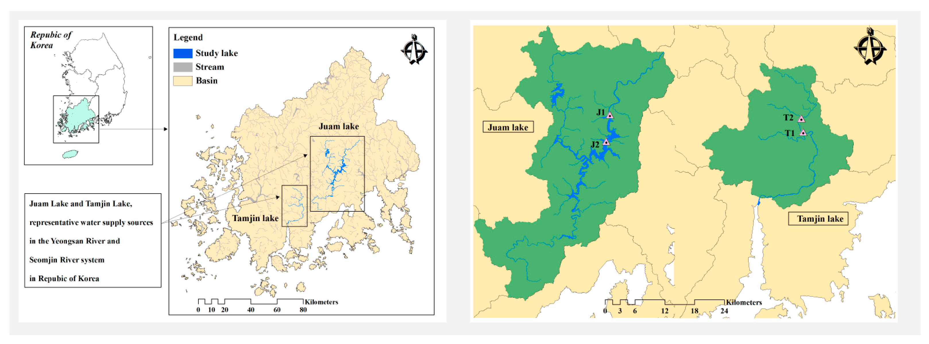
2.1. Study Area
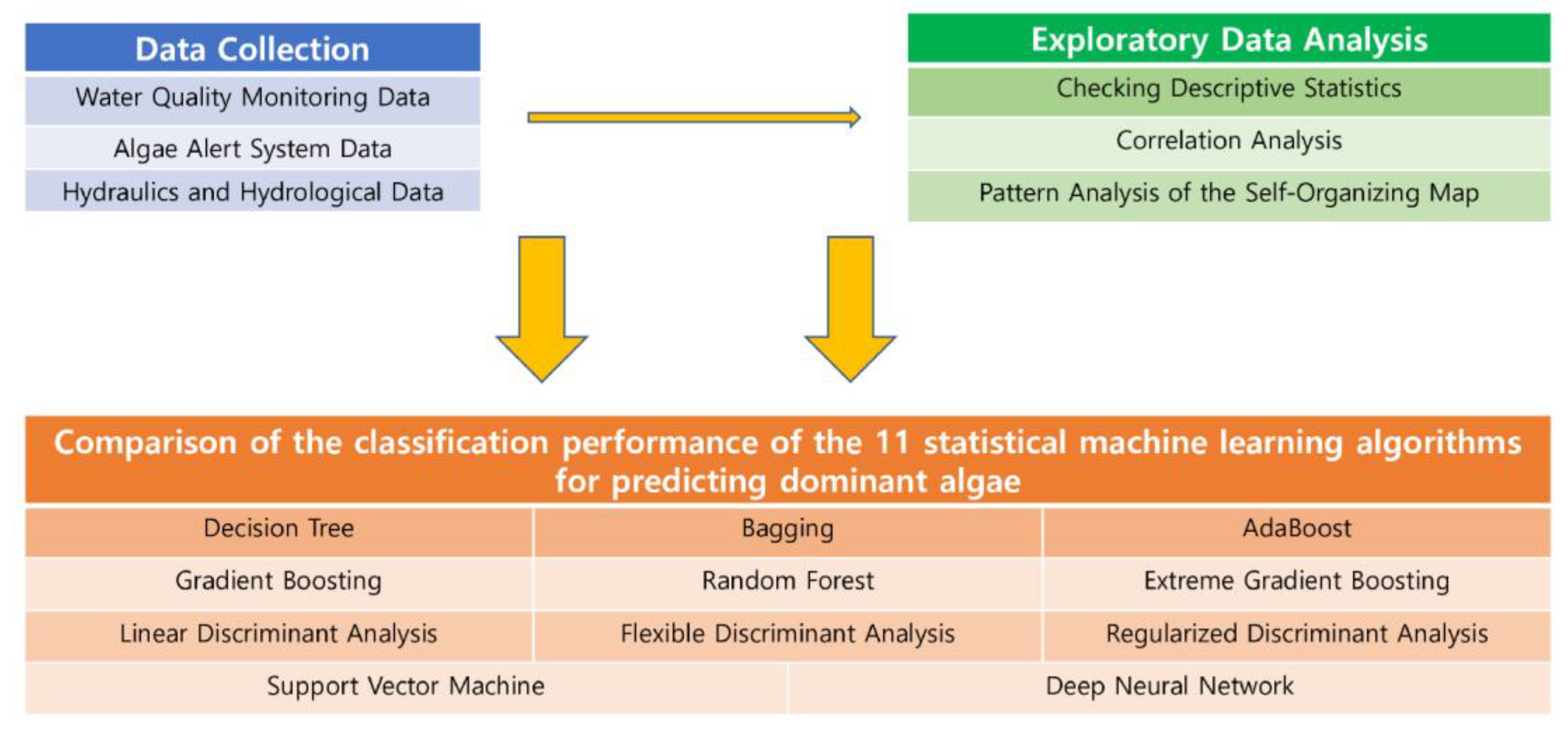
2.2. Data Collection
2.3. Data Analysis Methods
2.3.1. Exploratory Data Analysis
- Correlation analysis
- 2.
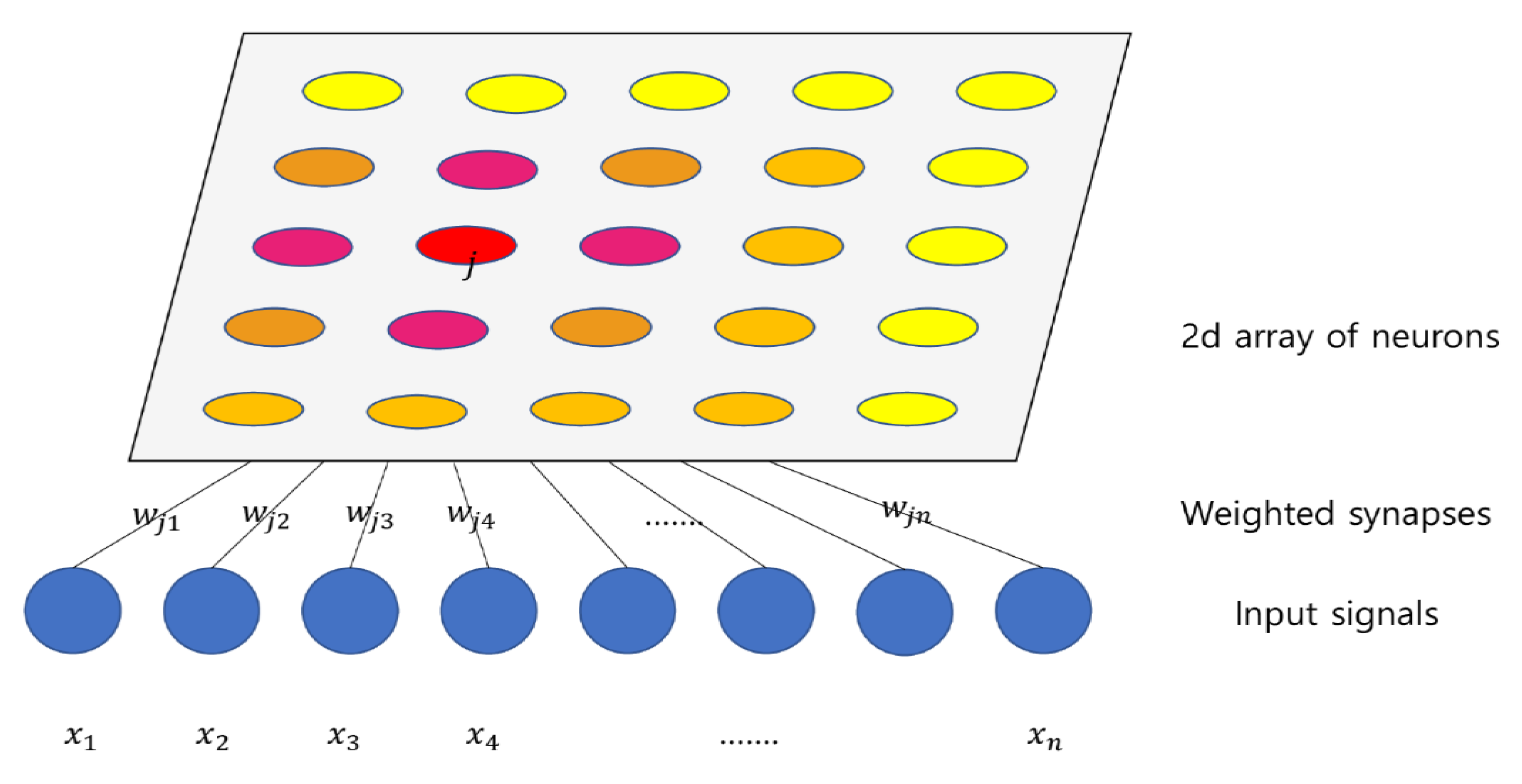
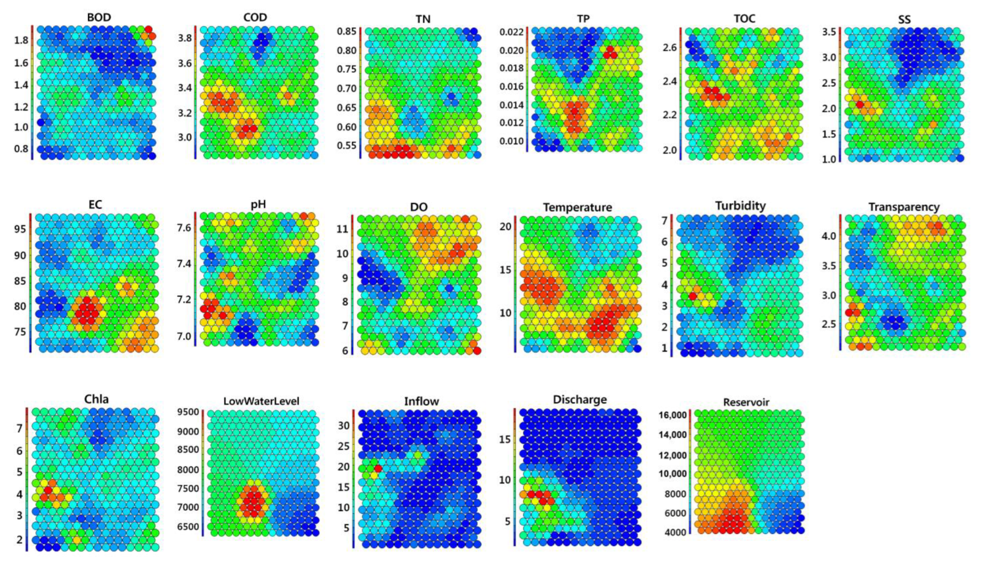
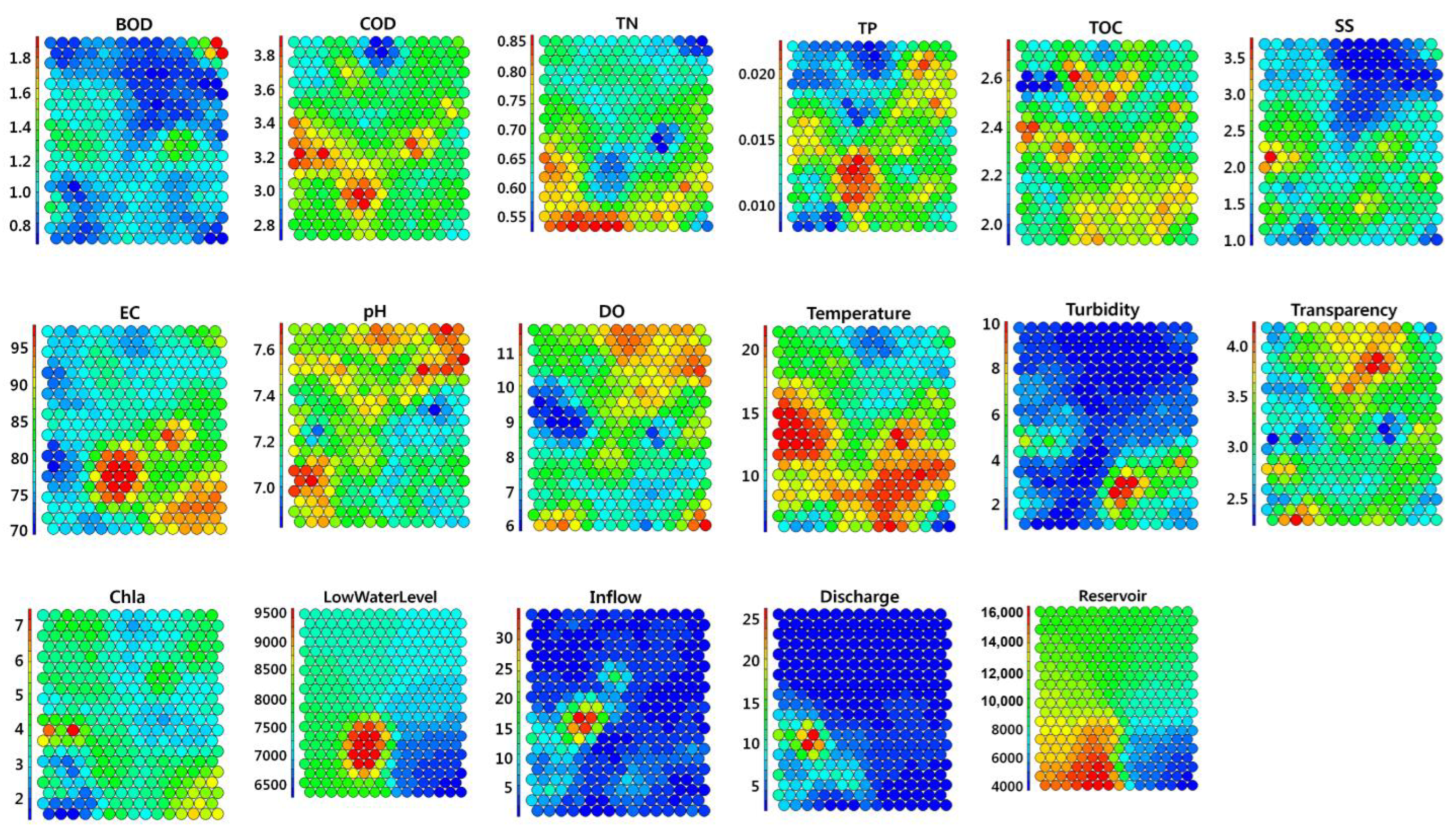
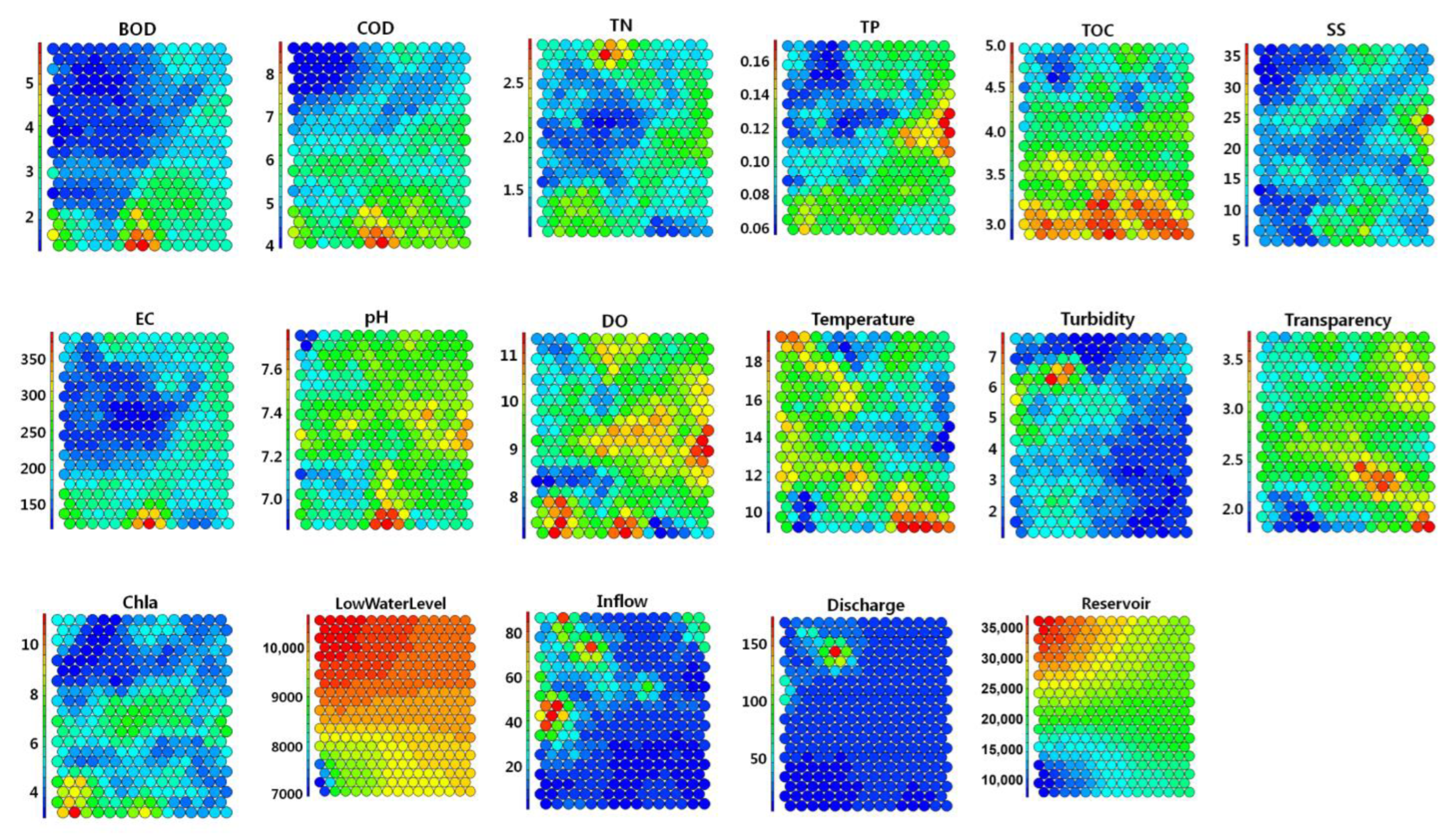
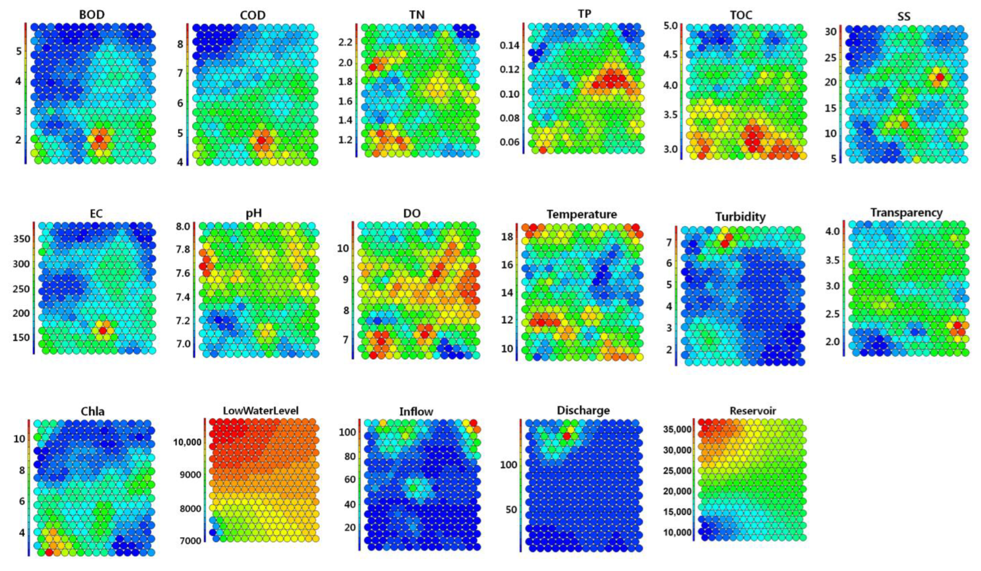
- Pattern analysis using SOM
2.3.2. Statistical Machine Learning Algorithms for Dominant Algal Classification
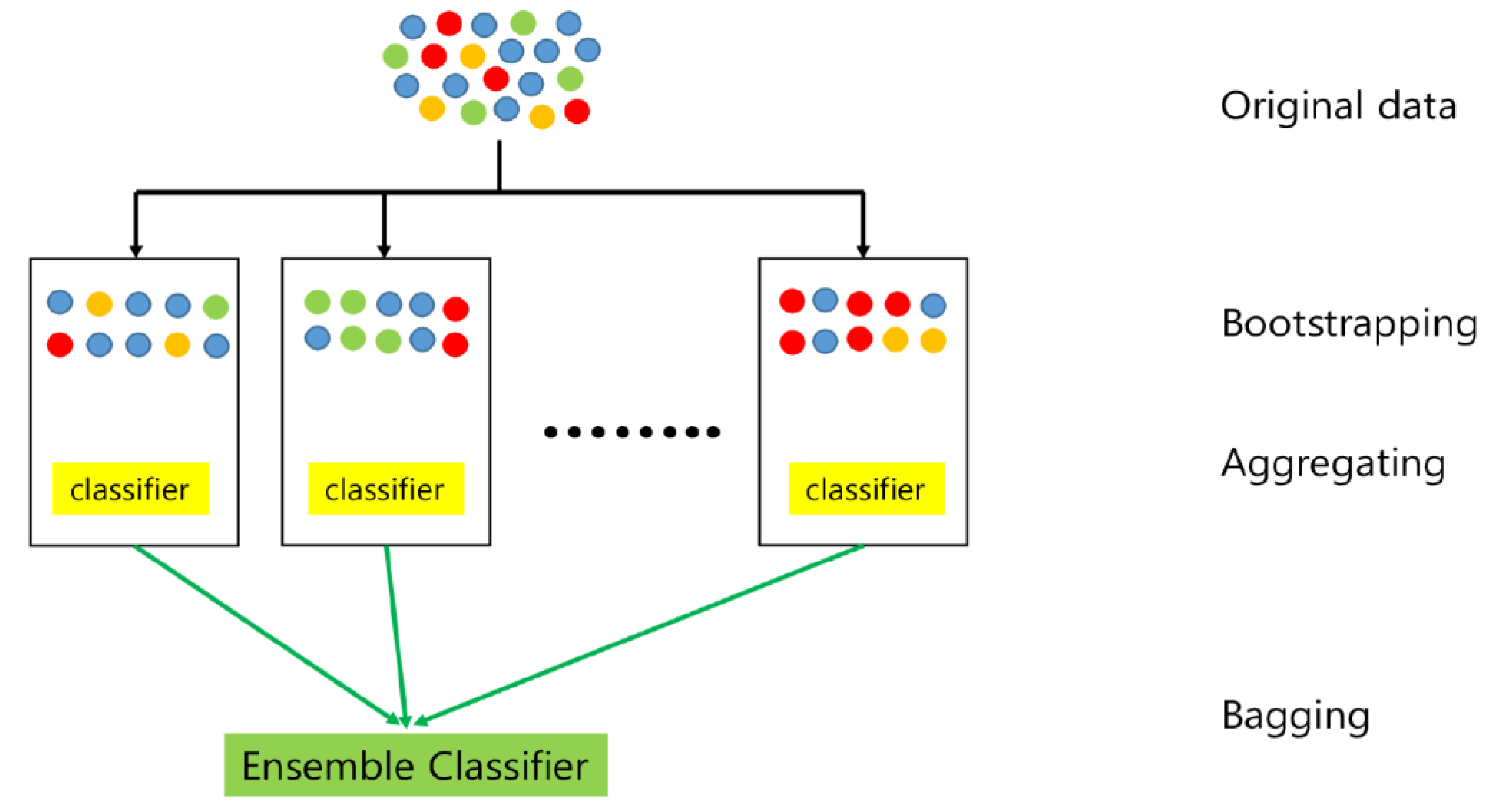
- Three tree-based methods
- 2.
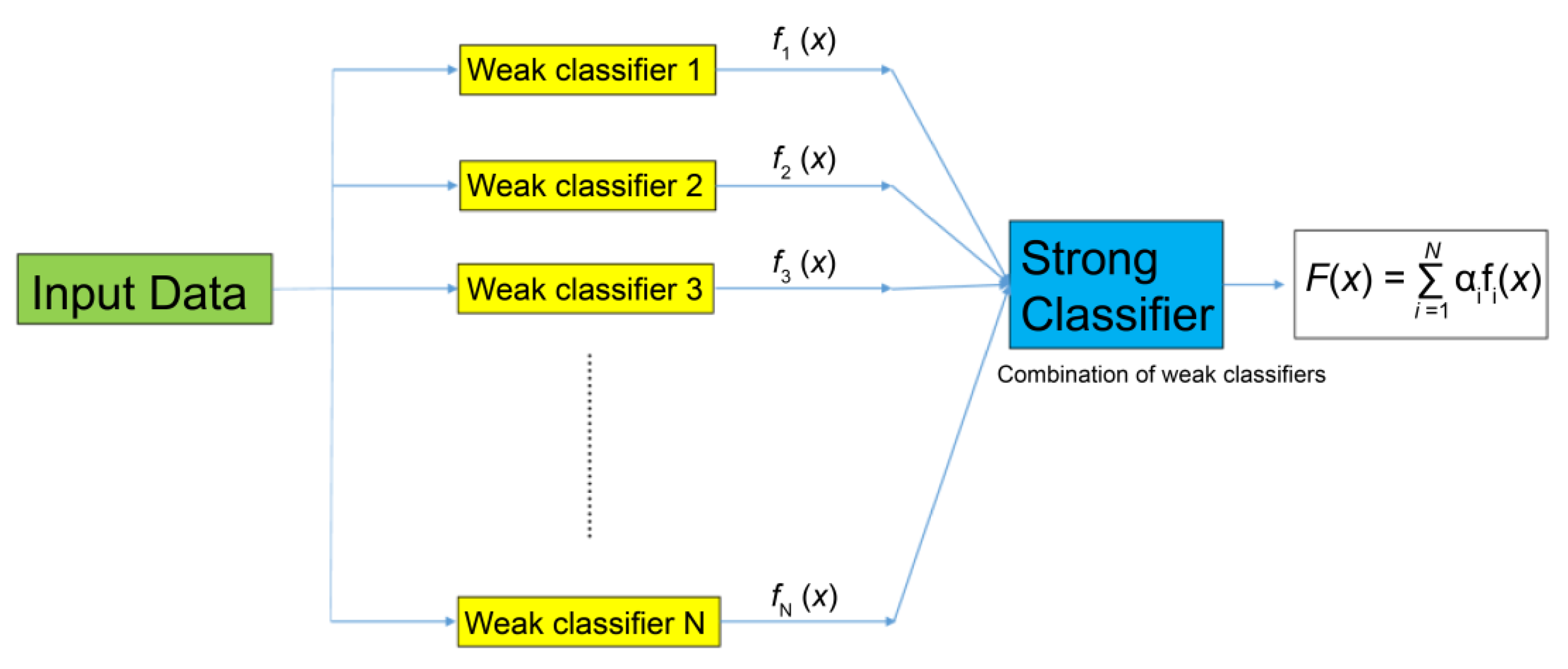
- AdaBoost (Ada)
- 3.
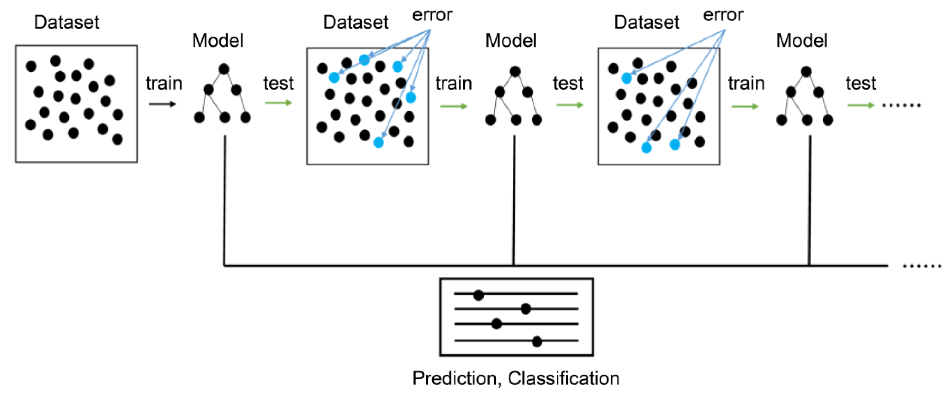
- Two gradient boosting methods
- 4.
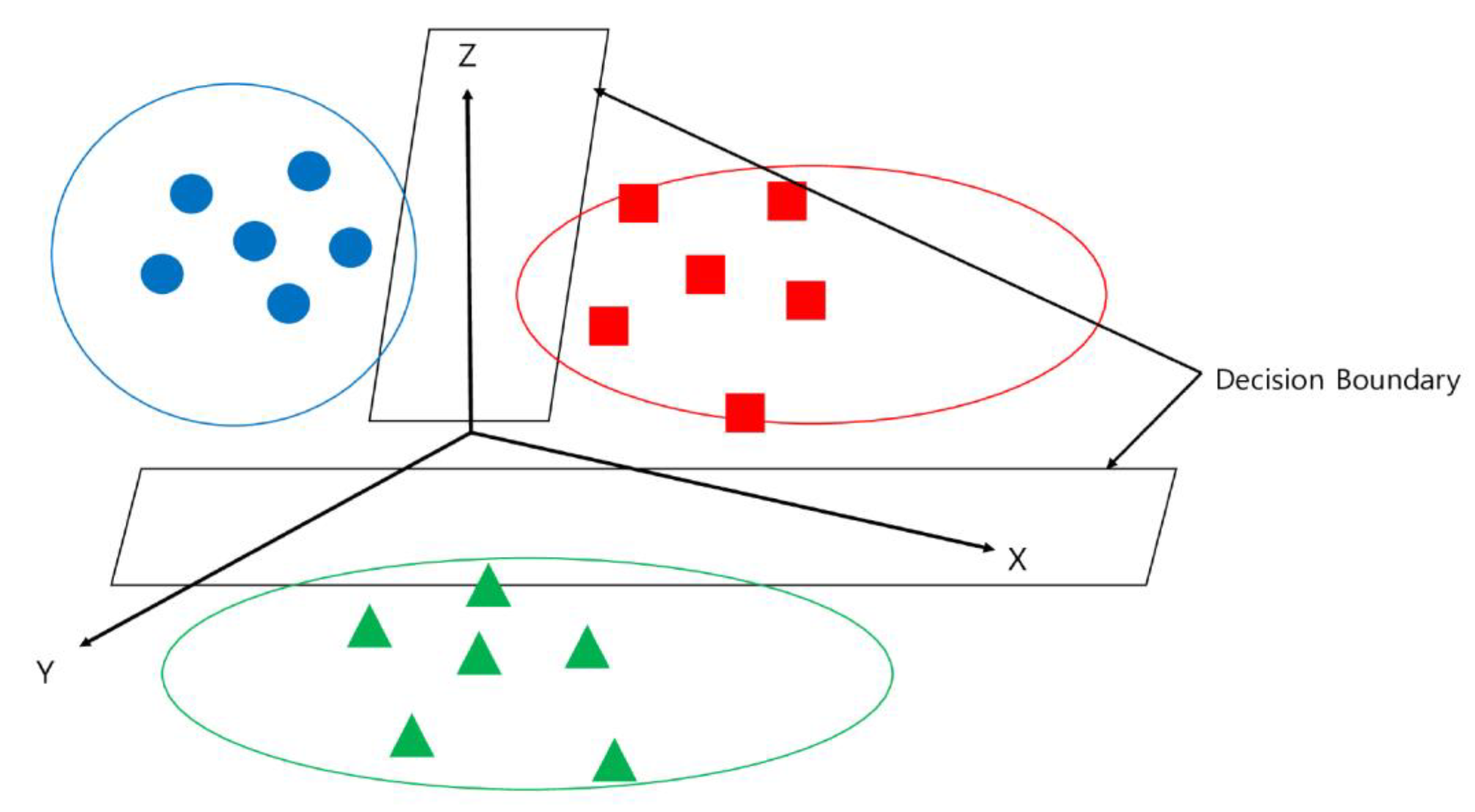
- Three discriminant analysis methods
- 5.
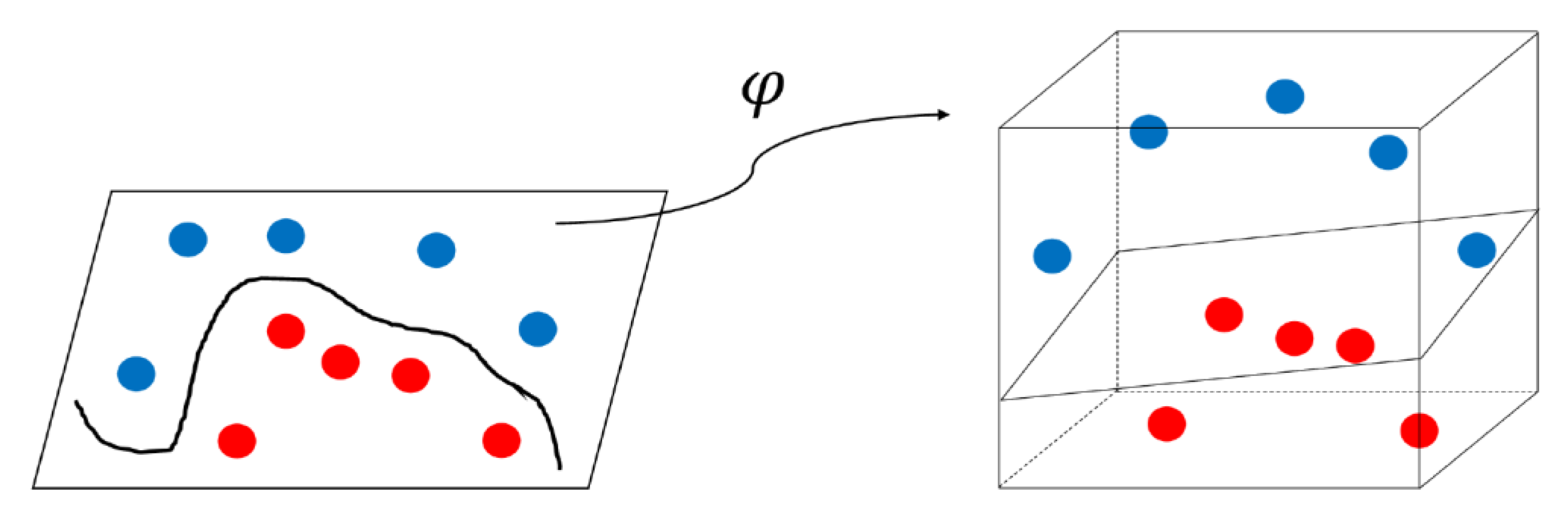
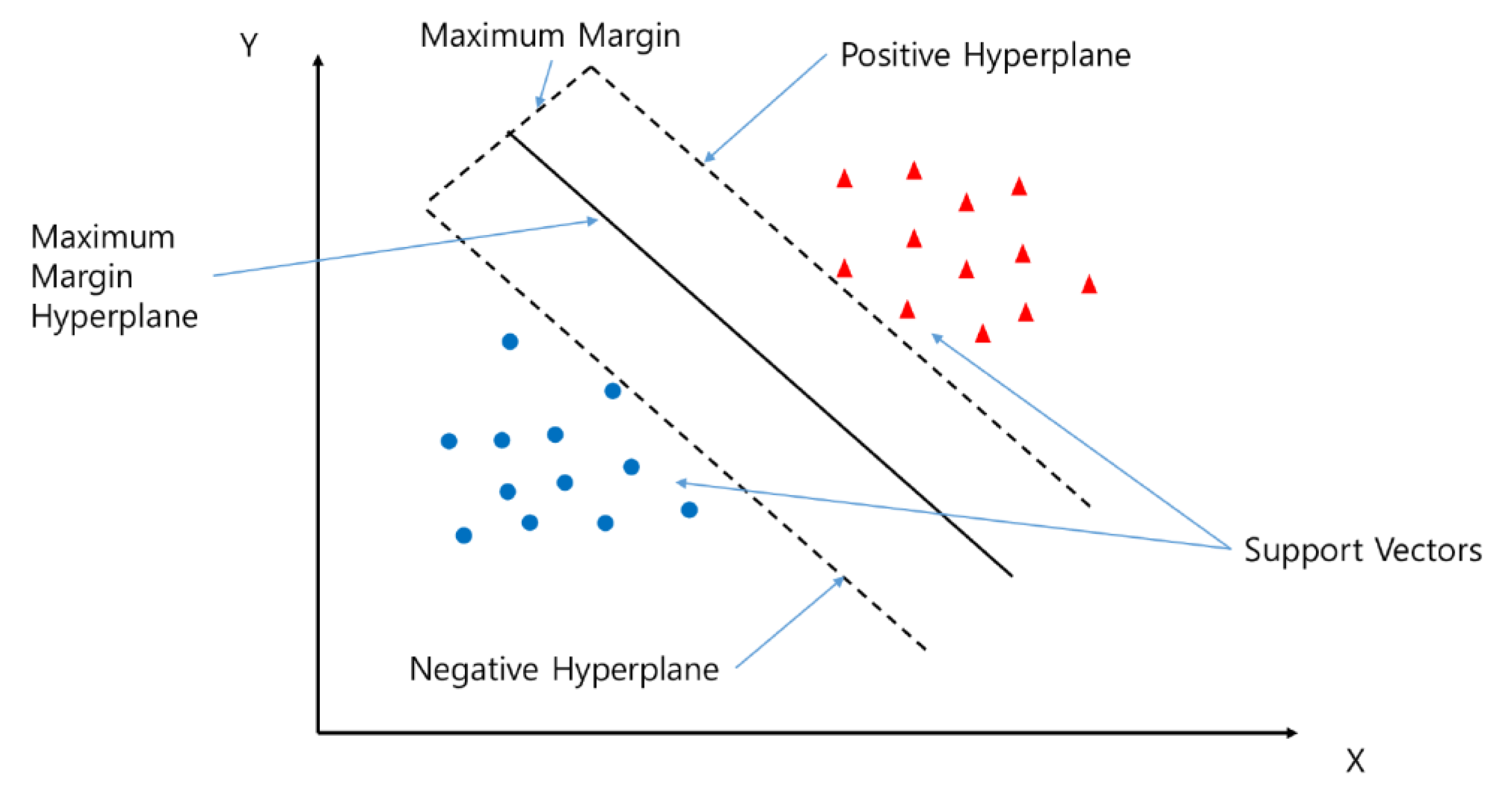
- Support Vector Machine (SVM)
- 6.
- Deep Neural Network (DNN)
2.3.3. Evaluation Indexes
3. Results
3.1. Data Analysis
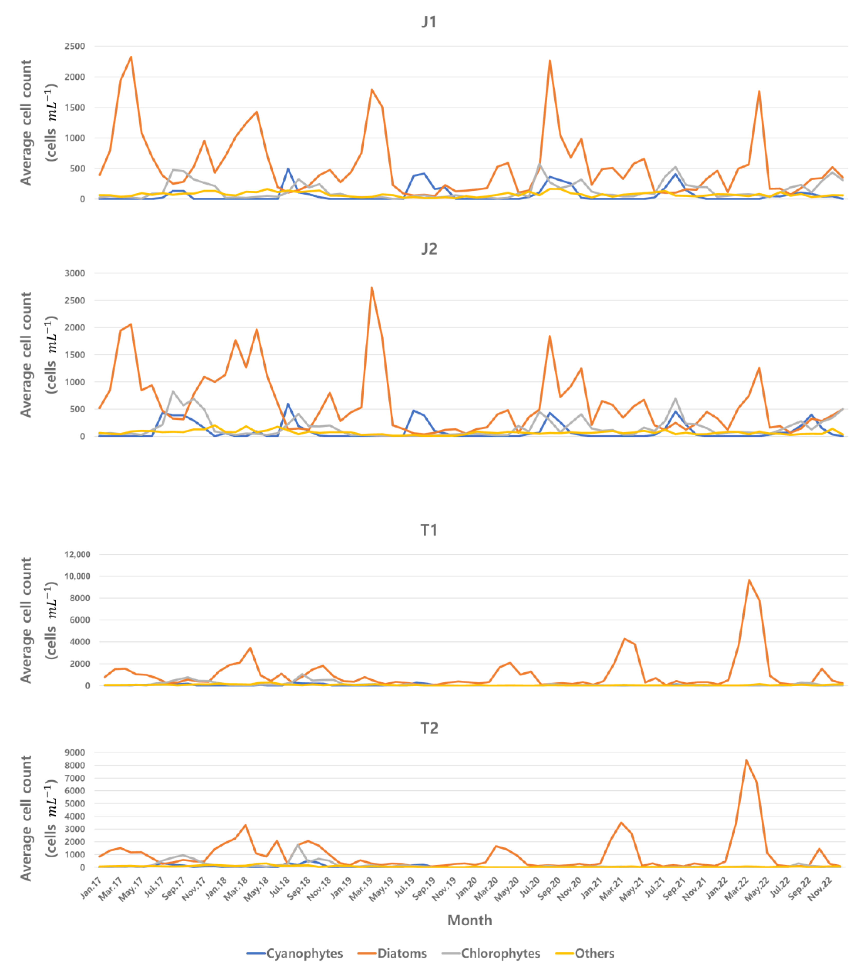
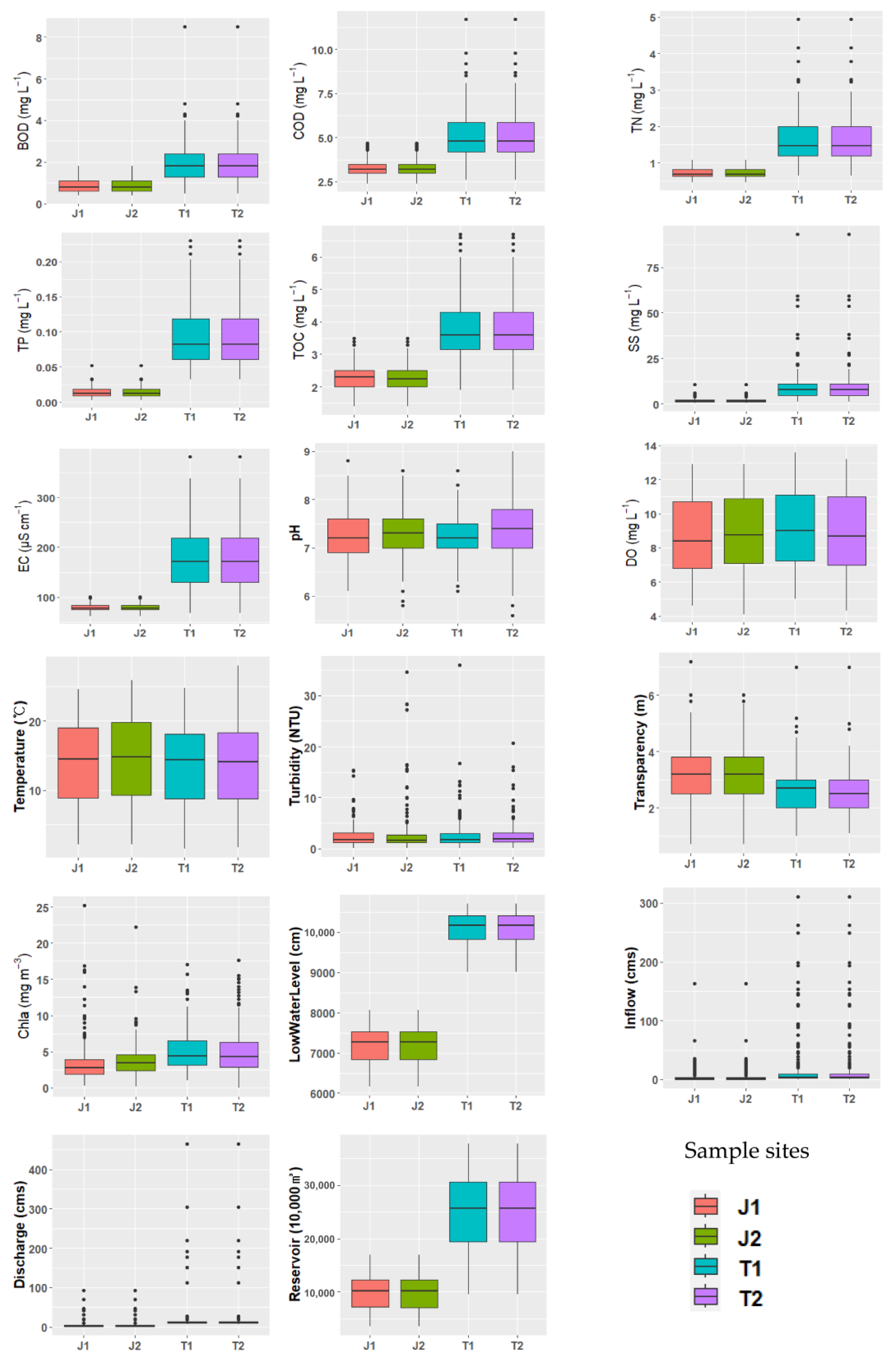
3.1.1. Exploratory Data Analysis for Monitoring Data
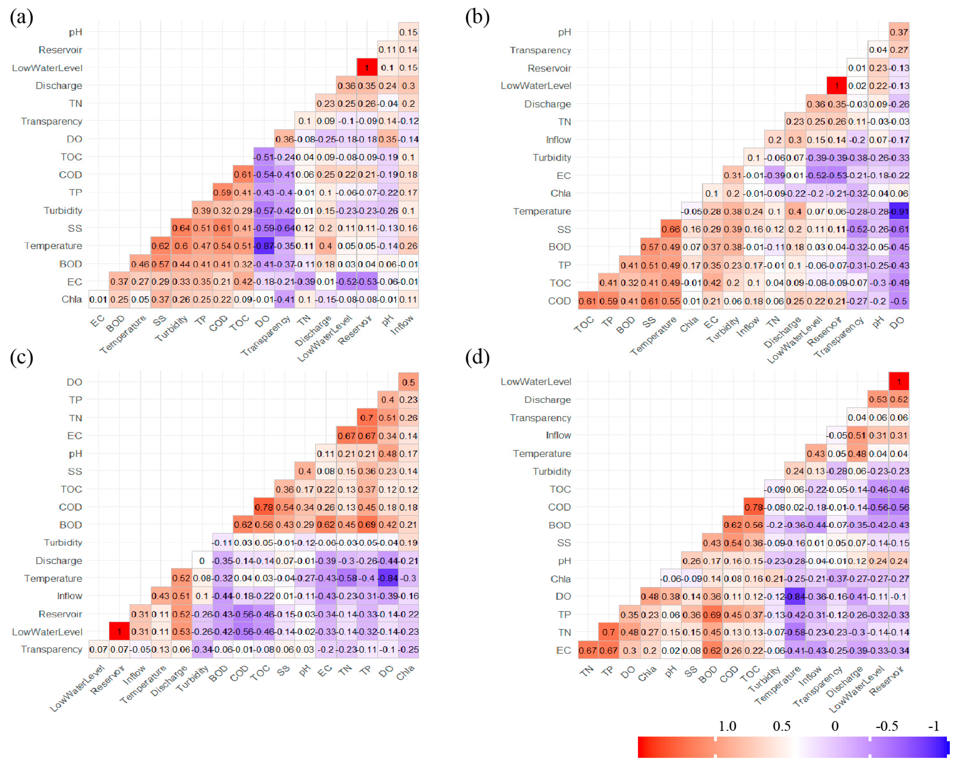
3.1.2. Correlation Analysis and SOM Pattern Analysis
3.2. Comparison of the Performance of the Statistical Machine Learning Algorithms
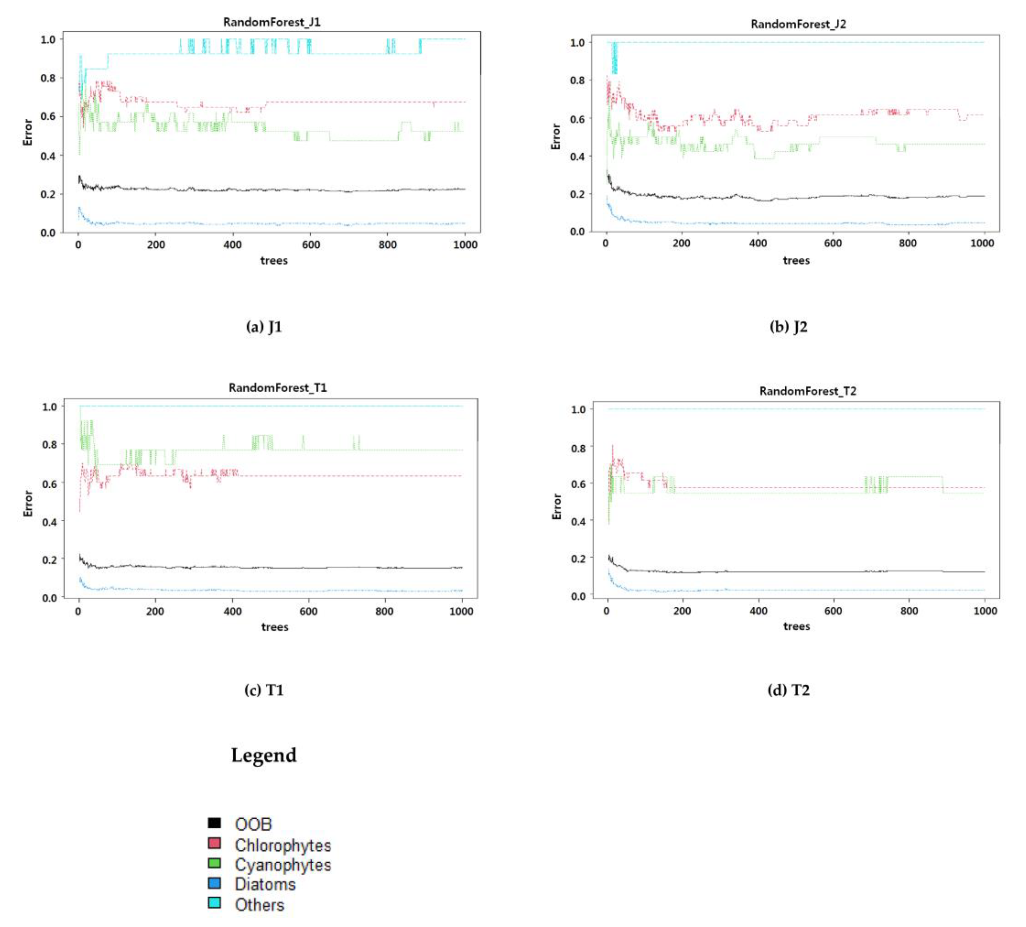
3.2.1. Tree-Based Algorithm for Assessing Variable Importance
3.2.2. Comparison of Algorithms Based on Four Criteria
4. Discussion
5. Conclusions
Author Contributions
Funding
Data Availability Statement
Acknowledgments
Conflicts of Interest
References
- Kim, S.G. Green algae and algae warning system. Water Future 2017, 50, 22–26. [Google Scholar]
- Kim, K.B.; Jung, M.K.; Tsang, Y.F.; Kwon, H.H. Stochastic modeling of chlorophyll-a for probabilistic assessment and monitoring of algae blooms in the Lower Nakdong River, South Korea. J. Hazard. Mater. 2020, 400, 123066. [Google Scholar] [CrossRef] [PubMed]
- Srivastava, A.; Ahn, C.Y.; Asthana, R.K.; Lee, H.G.; Oh, H.M. Status, alert system, and prediction of cyanobacterial bloom in South Korea. Biomed. Res. Int. 2015, 2015, 584696. [Google Scholar] [CrossRef] [PubMed] [Green Version]
- Falconer, I.R.; Humpage, A.R. Health risk assessment of cyanobacterial (blue-green algal) toxins in drinking water. Int. J. Environ. Res. Public Health 2005, 2, 43–50. [Google Scholar] [CrossRef] [Green Version]
- Fleming, L.E.; Rivero, C.; Burns, J.; Williams, C.; Bean, J.A.; Shea, K.A.; Stinn, J. Blue green algal (cyanobacterial) toxins, surface drinking water, and liver cancer in Florida. Harmful Algae 2002, 1, 157–168. [Google Scholar] [CrossRef]
- Kim, Y.H. Harmful Cyanobacterial Bloom and Application of Physical, Chemical and Biological Control Methods. Ph.D. Thesis, Hanyang University, Seoul, Republic of Korea, 2022. [Google Scholar]
- Joo, J.H. Field Application and Development of Biologically Derived Substances (BDSs) to Mitigate Freshwater Harmful Cyanobacterial Blooms. Ph.D. Thesis, Hanyang University, Seoul, Republic of Korea, 2017. [Google Scholar]
- Guillaume, M.C.; Dos Santos, F.B. Assessing and reducing phenotypic instability in cyanobacteria. Curr. Opin. Biotechnol. 2023, 80, 102899. [Google Scholar] [CrossRef]
- Kim, H.G. Prediction of Chlorophyll-A in the Middle Reach of the Nakdong River at Maegok Using Artificial Neural Networks. Master’s Thesis, Department of Integrated Biological Science, The Graduate School of Busan National University, Busan, Republic of Korea, 2017. [Google Scholar]
- Lee, S.M.; Park, K.D.; Kim, I.K. Comparison of machine learning algorithms for Chl-a prediction in the middle of Nakdong river (focusing on water quality and quantity factors). J. Korean Soc. Water Wastewater 2020, 34, 277–288. [Google Scholar] [CrossRef]
- Bui, D.T.; Khosravi, K.; Tiefenbacher, J.; Nguyen, H.; Kazakis, N. Improving prediction of water quality indices using novel hybrid machine-learning algorithms. Sci. Total Environ. 2020, 721, 137612. [Google Scholar] [CrossRef]
- Caissie, D.; Satish, M.G.; El-Jabi, N. Predicting water temperatures using a deterministic model: Application on Miramichi River catchments (New Brunswick, Canada). J. Hydrol. 2007, 336, 303–315. [Google Scholar] [CrossRef]
- Choi, D.H.; Jung, J.W.; Lee, K.S.; Choi, Y.J.; Yoon, K.S.; Cho, S.H.; Park, H.N.; Lim, B.J.; Chang, N.I. Estimation of pollutant load delivery ratio for flow duration using LQ equation from the Oenam-cheon watershed in Juam Lake. J. Environ. Sci. Int. 2012, 21, 31–39. [Google Scholar] [CrossRef]
- Park, H.G.; Kang, D.W.; Shin, K.H.; Ock, G.Y. Tracing source and concentration of riverine organic carbon transporting from Tamjin River to Gangjin Bay, Korea. KJEE 2017, 50, 422–431. [Google Scholar] [CrossRef]
- Seo, K.A.; Jung, S.J.; Park, J.H.; Hwang, K.S.; Lim, B.J. Relationships between the Characteristics of Algae Occurrence and Environmental Factors in Lake Juam, Korea. J. Korean Soc. Water Environ. 2013, 29, 317–328. [Google Scholar]
- Cox, V. Exploratory data analysis. In Translating Statistics to Make Decisions; Apress: Berkeley, CA, USA, 2017; pp. 47–74. [Google Scholar]
- Das, K.R.; Imon, A.H.M.R. A brief review of tests for normality. Am. J. Ther. Appl. Stat. 2016, 5, 5–12. [Google Scholar] [CrossRef] [Green Version]
- Thadewald, T.; Büning, H. Jarque–Bera test and its competitors for testing normality—A power comparison. J. Appl. Stat. 2007, 34, 87–105. [Google Scholar] [CrossRef]
- Kohonen, T. The self-organizing map. Proc. IEEE 1990, 78, 1464–1480. [Google Scholar] [CrossRef]
- Jung, K.Y.; Cho, S.H.; Hwang, S.Y.; Lee, Y.J.; Kim, K.H.; Na, E.H. Identification of High-Priority Tributaries for Water Quality Management in Nakdong River Using Neural Networks and Grade Classification. Sustainability 2020, 12, 9149. [Google Scholar] [CrossRef]
- James, G.; Witten, D.; Hastie, T.; Tibshirani, R. An Introduction to Statistical Learning; Springer: New York, NY, USA, 2013; Volume 112, p. 18. [Google Scholar]
- Sugiyama, M. Introduction to Statistical Machine Learning; Morgan Kaufmann: Burlington, MA, USA, 2015. [Google Scholar]
- Park, K.Y.; JW, K. A short guide to machine learning for economists. Korean J. Econ. 2019, 26, 367–408. [Google Scholar] [CrossRef]
- Han, S.W. A Study on Kernel Ridge Regression Using Ensemble Method. Master’s Thesis, Department of Statistics, The Graduate School of Hankuk University of Foreign Studies, Seoul, Republic of Korea, 2016. [Google Scholar]
- Hwang, S.Y. A Study on Efficiency of Kernel Ridge Logistic Regression Classification Using Ensemble Method. Master’s Thesis, Department of Statistics, The Graduate School of Hankuk University of Foreign Studies, Seoul, Republic of Korea, 2017. [Google Scholar]
- Cutler, A.; Cutler, D.R.; Stevens, J.R. Random forests. In Ensemble Machine Learning; Springer: Boston, MA, USA, 2012; pp. 157–175. [Google Scholar]
- Schapire, R.E. Explaining adaboost. In Empirical Inference; Springer: Berlin/Heidelberg, Germany, 2013; pp. 37–52. [Google Scholar]
- Natekin, A.; Knoll, A. Gradient boosting machines, a tutorial. Front. Neurorobot. 2013, 7, 21. [Google Scholar] [CrossRef] [Green Version]
- Chen, T.; He, T.; Benesty, M.; Khotilovich, V.; Tang, Y.; Cho, H.; Chen, K. Xgboost: Extreme Gradient Boosting, R Package Version 0.4-2. 2015, pp. 1–4. Available online: https://cran.microsoft.com/snapshot/2017-12-11/web/packages/xgboost/vignettes/xgboost.pdf (accessed on 10 January 2023).
- Izenman, A.J. Linear discriminant analysis. In Modern Multivariate Statistical Techniques; Springer: New York, NY, USA, 2013; pp. 237–280. [Google Scholar]
- Reynès, C.; Sabatier, R.; Molinari, N. Choice of B-splines with free parameters in the flexible discriminant analysis context. Comput. Stat. Data Anal. 2006, 51, 1765–1778. [Google Scholar] [CrossRef]
- Schölkopf, B.; Smola, A.J.; Williamson, R.C.; Bartlett, P.L. New support vector algorithms. Neural Comput. 2000, 12, 1207–1245. [Google Scholar] [CrossRef]
- Friedman, J.H. Regularized discriminant analysis. J. Am. Stat. Assoc. 1989, 84, 165–175. [Google Scholar] [CrossRef]
- Pisner, D.A.; Schnyer, D.M. Support vector machine. In Machine Learning; Academic Press: Cambridge, MA, USA, 2020; pp. 101–121. [Google Scholar]
- Montavon, G.; Samek, W.; Müller, K.R. Methods for interpreting and understanding deep neural networks. Digit Signal Process. 2018, 73, 1–15. [Google Scholar] [CrossRef]
- Parikh, R.; Mathai, A.; Parikh, S.; Sekhar, G.C.; Thomas, R. Understanding and using sensitivity, specificity and predictive values. Indian J. Ophthalmol. 2008, 56, 45. [Google Scholar] [CrossRef] [PubMed]
- Xu, J.; Zhang, Y.; Miao, D. Three-way confusion matrix for classification: A measure driven view. Inf. Sci. 2020, 507, 772–794. [Google Scholar] [CrossRef]
- Li, D.L.; Shen, F.; Yin, Y.; Peng, J.X.; Chen, P.Y. Weighted Youden index and its two-independent-sample comparison based on weighted sensitivity and specificity. Chin. Med. J. 2013, 126, 1150–1154. [Google Scholar]
- Trevethan, R. Sensitivity, specificity, and predictive values: Foundations, pliabilities, and pitfalls in research and practice. Front. Public Health 2017, 5, 307. [Google Scholar] [CrossRef]
- Jung, K.Y.; Lee, I.J.; Lee, K.L.; Cheon, S.U.; Hong, J.Y.; Ahn, J.M. Long-term trend analysis and exploratory data analysis of Geumho River based on seasonal Mann-Kendall test. J. Environ. Sci. Int. 2016, 25, 217–229. [Google Scholar] [CrossRef]
- Blanca, M.J.; Arnau, J.; López-Montiel, D.; Bono, R.; Bendayan, R. Skewness and kurtosis in real data samples. Methodology 2013, 9, 78–84. [Google Scholar] [CrossRef]
- De Winter, J.C.; Gosling, S.D.; Potter, J. Comparing the Pearson and Spearman correlation coefficients across distributions and sample sizes: A tutorial using simulations and empirical data. Psychol. Methods 2016, 21, 273. [Google Scholar] [CrossRef] [PubMed]
- Bai, J.; Ng, S. Tests for skewness, kurtosis, and normality for time series data. J. Bus. Econ. Stat. 2005, 23, 49–60. [Google Scholar] [CrossRef] [Green Version]
- Gregorutti, B.; Michel, B.; Saint-Pierre, P. Correlation and variable importance in random forests. Stat. Comput. 2017, 27, 659–678. [Google Scholar] [CrossRef] [Green Version]
- Genuer, R.; Poggi, J.M. Random forests. In Random Forests with R; Springer: Cham, Switzerland, 2020; pp. 33–55. [Google Scholar]
- Roelofs, R.; Shankar, V.; Recht, B.; Fridovich-Keil, S.; Hardt, M.; Miller, J.; Schmidt, L. A meta-analysis of overfitting in machine learning. In Proceedings of the Advances in Neural Information Processing Systems 32 (NeurIPS 2019), Vancouver, BC, Canada, 8–14 December 2019. [Google Scholar]
- Woo, C.Y.; Yun, S.L.; Kim, S.G.; Lee, W.T. Occurrence of Harmful Blue-green Algae at Algae Alert System and Water Quality Forecast System Sites in Daegu and Gyeongsangbuk-do between 2012 and 2019. J. Korean Soc. Environ. Eng. 2020, 42, 664–673. [Google Scholar] [CrossRef]
- Jung, K.Y.; Ahn, J.M.; Kim, K.; Lee, I.J.; Yang, D.S. Evaluation of water quality characteristics and water quality improvement grade classification of Geumho River tributaries. J. Environ. Sci. Int. 2016, 25, 767–787. [Google Scholar] [CrossRef]
- Sun, X.; Zhang, H.; Zhong, M.; Wang, Z.; Liang, X.; Huang, T.; Huang, H. Analyses on the temporal and spatial characteristics of water quality in a seagoing river using multivariate statistical techniques: A case study in the Duliujian River, China. Int. J. Environ. Res. Public Health 2019, 16, 1020. [Google Scholar] [CrossRef] [Green Version]


| Response Variable (Categorical) | Explanatory Variables (Continuous) | |
|---|---|---|
| Dominant Algae (Based on Total Cell Count) | Water Quality | Hydraulic/Hydrological |
| Cyanophytes Diatoms Chlorophytes Others | Biological Oxygen Demand (BOD), mg L−1 Chemical Oxygen Demand (COD), mg L−1 Total Nitrogen (TN), mg L−1 Total Phosphorus (TP), mg L−1 Total Organic Carbon (TOC), mg L−1 Suspended Solids (SS), mg L−1 Electrical Conductivity (EC), μS L−1 pH Dissolved Oxygen (DO), mg L−1 Temperature, °C Turbidity, NTU Transparency, m Chlorophyll a (Chla), mg m−3 | Low Water Level, cm Inflow Rate (Inflow), cms Discharge Rate (Discharge), cms Water Storage Capacity (Reservoir), 10,000 m3 |
| Cyanophytes | Diatoms | Chlorophytes | Others | |
|---|---|---|---|---|
| Normal | Harmful | |||
| Aphanocapsa Chroococcus Merismopedia Phormidium Pseudanabaena Worinochinia | Anabaena Aphanizomenon Microcystis Oscillatoria | Acanthoceras Achnanthes Asterionella Attheya Aulacoseira Coccoineis Cyclotella Cymbella Fragilaria Gomphonema Melosira Navicula Nitzschia Rhizosolenia Stephanodiscus Surirella Synedra | Actinastrum Ankistrodesmus Ankyra Chlamydomonas Chlorella Chodatella Closteriopsis Closterium Coelastrum Coenochloris Cosmarium Crucigenia Dictyosphaerium Dimorphococcus Elakatothrix Euastrum Eudorina Eunotia Gloeocystis Golenkinia Gonium Kirchnerionella Micractinium Monoraphidium Mougeotia Nephrocystium Oocystis Pandorina Pectodictyon Pediastrum Scenedesmus Schroederia Selenastrum Sphaerocystis Spondylosium Staurastrum Tetraedron Tetrastrum Treubaria | Ceratium Cryptomonas Dinobryon Euglena Kephyrion Mallomonas Peridinium Phacus Strombomonas Trachelomonas |
| Predicted | |||||
|---|---|---|---|---|---|
| Cyanophytes | Diatoms | Chlorophytes | Others | ||
| Actual | Cyanophytes | ||||
| Diatom | |||||
| Chlorophytes | |||||
| Others | |||||
| Predicted | |||
|---|---|---|---|
| Positive | Negative | ||
| Actual | Positive | True Positive (TP) | False Negative (FN) |
| Negative | False Positive (FP) | True Negative (TN) | |
| Survey Site | Statistics | BOD | COD | TN | TP | TOC | SS | EC | pH | DO | Temperature (°C) | Turbidity (NTU) | Transparency (m) | Chla | Low Water Level (cm) | Inflow (cms) | Discharge (cms) | Reservoir (10,000 m3) |
|---|---|---|---|---|---|---|---|---|---|---|---|---|---|---|---|---|---|---|
| J1 | mean | 0.9500 | 3.3000 | 0.6800 | 0.0100 | 2.3400 | 1.8000 | 81.8000 | 7.2600 | 8.6200 | 14.1600 | 2.3200 | 3.1700 | 3.3300 | 7260.4900 | 3.6100 | 4.1200 | 9945.4800 |
| sd | 0.3800 | 0.4300 | 0.1300 | 0.0100 | 0.4100 | 1.0400 | 8.8200 | 0.4300 | 2.2200 | 5.6300 | 2.0100 | 1.0000 | 2.6900 | 620.7500 | 11.3300 | 7.7000 | 3298.5100 | |
| median | 0.9000 | 3.3000 | 0.6600 | 0.0100 | 2.3000 | 1.5000 | 80.0000 | 7.2000 | 8.5000 | 14.7000 | 1.7000 | 3.2000 | 2.7000 | 7238.0000 | 0.8000 | 2.7000 | 9968.0000 | |
| min | 0.4000 | 2.4000 | 0.4400 | 0.0000 | 1.4000 | 0.5000 | 62.0000 | 6.1000 | 4.6000 | 2.1000 | 0.1000 | 0.7000 | 0.3000 | 6167.0000 | 0.0000 | 1.7000 | 3552.0000 | |
| max | 2.6000 | 4.7000 | 1.0800 | 0.0500 | 3.5000 | 10.6000 | 101.0000 | 8.8000 | 12.9000 | 24.6000 | 15.4000 | 7.2000 | 25.2000 | 9638.6200 | 162.6300 | 93.2100 | 16947.0000 | |
| skewness | 1.3100 | 0.5900 | 0.3800 | 1.1300 | 0.8600 | 3.1000 | 0.4500 | 0.1200 | 0.0700 | −0.0900 | 3.0800 | 0.2700 | 3.6000 | 1.4300 | 9.9200 | 8.2600 | 0.0500 | |
| kurtosis | 2.4400 | 0.1900 | −0.4500 | 2.4900 | 0.4700 | 17.9200 | −0.7600 | 0.0300 | −1.3300 | −1.3000 | 14.7300 | 0.4000 | 19.1600 | 4.0500 | 127.3000 | 78.2200 | −0.6800 | |
| JB test p-value | 0.0000 | 0.0001 | 0.0071 | 0.0000 | 0.0000 | 0.0000 | 0.0002 | 0.6839 | 0.0000 | 0.0000 | 0.0000 | 0.0517 | 0.0000 | 0.0000 | 0.0000 | 0.0000 | 0.0536 | |
| J2 | mean | 0.9500 | 3.3000 | 0.6800 | 0.0100 | 2.3400 | 1.8000 | 81.8000 | 7.3100 | 8.8000 | 14.8300 | 2.4300 | 3.1200 | 3.7200 | 7260.4900 | 3.6100 | 4.1200 | 9945.4800 |
| sd | 0.3800 | 0.4300 | 0.1300 | 0.0100 | 0.4100 | 1.0400 | 8.8200 | 0.4500 | 2.1700 | 6.0000 | 3.5800 | 0.9300 | 2.1600 | 620.7500 | 11.3300 | 7.7000 | 3298.5100 | |
| median | 0.9000 | 3.3000 | 0.6600 | 0.0100 | 2.3000 | 1.5000 | 80.0000 | 7.3000 | 8.8000 | 15.2000 | 1.6000 | 3.0000 | 3.4000 | 7238.0000 | 0.8000 | 2.7000 | 9968.0000 | |
| min | 0.4000 | 2.4000 | 0.4400 | 0.0000 | 1.4000 | 0.5000 | 62.0000 | 5.8000 | 4.1000 | 2.1000 | 0.1000 | 0.7000 | 0.2000 | 6167.0000 | 0.0000 | 1.7000 | 3552.0000 | |
| max | 2.6000 | 4.7000 | 1.0800 | 0.0500 | 3.5000 | 10.6000 | 101.0000 | 8.6000 | 12.9000 | 25.9000 | 34.6000 | 6.0000 | 22.2000 | 9638.6200 | 162.6300 | 93.2100 | 16947.0000 | |
| skewness | 1.3100 | 0.5900 | 0.3800 | 1.1300 | 0.8600 | 3.1000 | 0.4500 | −0.1600 | −0.0700 | −0.0800 | 5.6000 | 0.3400 | 2.9700 | 1.4300 | 9.9200 | 8.2600 | 0.0500 | |
| kurtosis | 2.4400 | 0.1900 | −0.4500 | 2.4900 | 0.4700 | 17.9200 | −0.7600 | 0.4200 | −1.1100 | −1.3100 | 38.0000 | 0.4300 | 18.6800 | 4.0500 | 127.3000 | 78.2200 | −0.6800 | |
| JB test p-value | 0.0000 | 0.0001 | 0.0071 | 0.0000 | 0.0000 | 0.0000 | 0.0002 | 0.1423 | 0.0004 | 0.0000 | 0.0000 | 0.0137 | 0.0000 | 0.0000 | 0.0000 | 0.0000 | 0.0536 | |
| T1 | mean | 2.2700 | 5.4100 | 1.6300 | 0.1000 | 3.8700 | 10.6300 | 185.9900 | 7.2700 | 9.1700 | 13.8100 | 2.4200 | 2.6300 | 5.1600 | 9908.6600 | 15.0100 | 17.0300 | 23247.5400 |
| sd | 1.3600 | 1.5700 | 0.6600 | 0.0400 | 1.0000 | 11.0200 | 65.1200 | 0.4200 | 2.1900 | 5.4700 | 2.8400 | 0.7300 | 2.9300 | 724.5500 | 39.1100 | 37.2400 | 8015.6200 | |
| median | 2.0000 | 5.0000 | 1.4700 | 0.0900 | 3.7000 | 8.4000 | 178.0000 | 7.3000 | 9.1000 | 14.5000 | 1.7000 | 2.6000 | 4.4000 | 10063.0000 | 3.7000 | 11.3800 | 23560.0000 | |
| min | 0.5000 | 2.6000 | 0.6400 | 0.0300 | 1.9000 | 1.3000 | 68.0000 | 6.1000 | 4.8000 | 1.5000 | 0.1000 | 1.0000 | 0.4000 | 6805.0000 | 0.0000 | 1.9400 | 7105.0000 | |
| max | 8.8000 | 13.0000 | 4.9400 | 0.2300 | 6.7000 | 93.2000 | 600.0000 | 8.6000 | 13.6000 | 24.8000 | 36.0000 | 7.0000 | 19.0000 | 10704.0000 | 310.6300 | 464.6000 | 37807.0000 | |
| skewness | 2.0100 | 1.3200 | 1.7500 | 0.9100 | 0.4900 | 4.0800 | 1.5300 | 0.1700 | 0.0300 | −0.1900 | 6.6500 | 1.0100 | 1.4100 | −2.5200 | 4.5800 | 8.5400 | −0.0800 | |
| kurtosis | 5.4200 | 2.5300 | 4.6100 | 0.1400 | −0.2500 | 20.9300 | 5.7900 | −0.0500 | −1.1300 | −1.0800 | 66.1100 | 3.8700 | 2.8500 | 8.1000 | 23.3700 | 83.5000 | −0.9600 | |
| JB test p-value | 0.0000 | 0.0000 | 0.0000 | 0.0000 | 0.0016 | 0.0000 | 0.0000 | 0.4793 | 0.0003 | 0.0003 | 0.0000 | 0.0000 | 0.0000 | 0.0000 | 0.0000 | 0.0000 | 0.0029 | |
| T2 | mean | 2.2700 | 5.4100 | 1.6300 | 0.1000 | 3.8700 | 10.6300 | 185.9900 | 7.3900 | 8.8400 | 13.7200 | 2.4100 | 2.5600 | 4.8700 | 9908.6600 | 15.0100 | 17.0300 | 23247.5400 |
| sd | 1.3600 | 1.5700 | 0.6600 | 0.0400 | 1.0000 | 11.0200 | 65.1200 | 0.5900 | 2.3400 | 5.5100 | 2.2400 | 0.7300 | 3.0400 | 724.5500 | 39.1100 | 37.2400 | 8015.6200 | |
| median | 2.0000 | 5.0000 | 1.4700 | 0.0900 | 3.7000 | 8.4000 | 178.0000 | 7.3000 | 8.7000 | 14.1500 | 1.8000 | 2.5000 | 4.1000 | 10063.0000 | 3.7000 | 11.3800 | 23560.0000 | |
| min | 0.5000 | 2.6000 | 0.6400 | 0.0300 | 1.9000 | 1.3000 | 68.0000 | 5.6000 | 4.1000 | 1.7000 | 0.1000 | 1.0000 | 0.0000 | 6805.0000 | 0.0000 | 1.9400 | 7105.0000 | |
| max | 8.8000 | 13.0000 | 4.9400 | 0.2300 | 6.7000 | 93.2000 | 600.0000 | 9.0000 | 13.2000 | 28.0000 | 20.7000 | 7.0000 | 17.6000 | 10704.0000 | 310.6300 | 464.6000 | 37807.0000 | |
| skewness | 2.0100 | 1.3200 | 1.7500 | 0.9100 | 0.4900 | 4.0800 | 1.5300 | −0.0100 | 0.0300 | −0.0400 | 4.0500 | 1.0900 | 1.2600 | −2.5200 | 4.5800 | 8.5400 | −0.0800 | |
| kurtosis | 5.4200 | 2.5300 | 4.6100 | 0.1400 | −0.2500 | 20.9300 | 5.7900 | 0.0300 | −1.1700 | −0.9600 | 23.3800 | 4.2200 | 1.7600 | 8.1000 | 23.3700 | 83.5000 | −0.9600 | |
| JB test p-value | 0.0000 | 0.0000 | 0.0000 | 0.0000 | 0.0016 | 0.0000 | 0.0000 | 0.9832 | 0.0002 | 0.0033 | 0.0000 | 0.0000 | 0.0000 | 0.0000 | 0.0000 | 0.0000 | 0.0029 |
| Survey Site | Cyanophytes | Diatoms | Chlorophytes | Others |
|---|---|---|---|---|
| J1 | 23 | 215 | 52 | 17 |
| J2 | 31 | 218 | 49 | 9 |
| T1 | 14 | 250 | 36 | 4 |
| T2 | 12 | 250 | 33 | 9 |
| Algorithm | Bagging | AdaBoost | Gradient Boosting | Random Forest | ||||||||||||
|---|---|---|---|---|---|---|---|---|---|---|---|---|---|---|---|---|
| Site | J1 | J2 | T1 | T2 | J1 | J2 | T1 | T2 | J1 | J2 | T1 | T2 | J1 | J2 | T1 | T2 |
| BOD | 1.5151 | 1.2076 | 1.4199 | 10.9415 | 5.3688 | 2.3051 | 3.2752 | 6.1182 | 4.4015 | 3.5559 | 3.6883 | 8.5063 | 5.9707 | 4.3431 | 3.6987 | 5.0601 |
| COD | 3.9329 | 0.6218 | 3.3253 | 0.9804 | 3.8681 | 4.3541 | 5.9501 | 6.1057 | 3.4951 | 2.4247 | 2.3878 | 3.2978 | 4.6970 | 3.5746 | 3.0373 | 2.7818 |
| TN | 7.6162 | 3.3504 | 4.7121 | 6.3081 | 7.1730 | 7.1124 | 4.8650 | 12.1125 | 6.8504 | 4.5037 | 3.9922 | 7.0974 | 6.9187 | 4.7123 | 5.0819 | 7.0660 |
| TP | 1.4593 | 0.9727 | 1.4096 | 1.7724 | 5.2335 | 5.1272 | 4.5811 | 5.5618 | 3.4535 | 2.7191 | 2.9967 | 3.0749 | 5.2055 | 4.1090 | 3.5175 | 3.0822 |
| TOC | 1.5957 | 1.0353 | 3.9916 | 2.2245 | 2.9938 | 3.6203 | 3.6343 | 5.8841 | 2.1803 | 2.9575 | 3.4477 | 4.5815 | 3.9918 | 4.1497 | 3.5106 | 3.6138 |
| SS | 1.7521 | 1.6342 | 2.6280 | 3.3955 | 6.5863 | 5.8286 | 7.2618 | 5.5634 | 4.9319 | 3.1961 | 5.3275 | 8.4605 | 6.3064 | 3.9993 | 3.9027 | 4.3123 |
| EC | 4.7823 | 3.7292 | 4.7572 | 2.3607 | 5.4583 | 4.9772 | 8.4684 | 6.4223 | 4.1840 | 3.5315 | 5.1276 | 4.0014 | 6.4564 | 4.5444 | 4.7248 | 3.4153 |
| pH | 4.7826 | 4.8354 | 0.6660 | 0.5151 | 4.7689 | 9.6268 | 3.5256 | 5.3030 | 5.3392 | 5.3432 | 1.4144 | 1.7538 | 5.1586 | 5.6326 | 2.6790 | 3.1063 |
| DO | 28.3646 | 3.9285 | 37.4578 | 1.2421 | 10.3830 | 7.9277 | 9.3204 | 3.2858 | 18.9131 | 11.9789 | 22.1672 | 3.7293 | 14.9578 | 12.9253 | 10.5199 | 4.7113 |
| Temperature | 26.6748 | 57.0166 | 4.5654 | 40.1099 | 8.7429 | 15.3805 | 11.5727 | 8.2058 | 15.4682 | 29.3555 | 8.6348 | 24.7510 | 14.2645 | 20.5988 | 6.3262 | 9.8519 |
| Turbidity | 1.3844 | 5.6681 | 1.8321 | 1.0291 | 5.9557 | 4.3917 | 7.1061 | 7.4450 | 3.7155 | 5.8834 | 3.8942 | 2.7514 | 5.3849 | 6.3450 | 3.1732 | 3.5382 |
| Transparency | 0.9296 | 0.8488 | 0.6438 | 6.6063 | 4.8024 | 3.5518 | 2.8340 | 3.3015 | 2.6789 | 1.4298 | 2.2568 | 3.0288 | 3.8831 | 3.3025 | 2.1322 | 2.5311 |
| Chla | 2.9024 | 2.9814 | 2.5859 | 10.6339 | 6.1437 | 6.5267 | 7.3452 | 11.5679 | 4.5390 | 5.3894 | 8.4450 | 8.2374 | 5.5247 | 4.8334 | 4.2982 | 5.5031 |
| Low Water Level | 5.4858 | 8.8656 | 24.4891 | 6.2134 | 8.3114 | 8.8755 | 6.2390 | 4.1642 | 6.4153 | 7.5803 | 11.3711 | 5.7199 | 6.4287 | 7.0199 | 6.3847 | 4.3711 |
| Inflow | 2.6177 | 1.5479 | 1.4467 | 1.2481 | 6.6966 | 5.5075 | 8.0738 | 3.6056 | 6.0363 | 5.1891 | 5.8343 | 3.6946 | 5.3530 | 4.3713 | 4.1482 | 2.3601 |
| Discharge | 3.9374 | 1.7066 | 2.8512 | 4.3660 | 7.0177 | 4.7818 | 5.0124 | 5.2433 | 6.4306 | 2.5860 | 7.2105 | 6.5851 | 7.6860 | 5.9045 | 5.4156 | 4.0187 |
| Reservoir | 0.2672 | 0.0500 | 1.2183 | 0.0531 | 0.4960 | 0.1051 | 0.9349 | 0.1097 | 0.9672 | 2.3757 | 1.8039 | 0.7290 | 6.6168 | 6.8222 | 6.0186 | 4.5432 |
| Method | Gain | Cover | Frequency | |||||||||
|---|---|---|---|---|---|---|---|---|---|---|---|---|
| Site | J1 | J2 | T1 | T2 | J1 | J2 | T1 | T2 | J1 | J2 | T1 | T2 |
| BOD | 0.0437 | 0.0191 | 0.0168 | 0.0817 | 0.0409 | 0.0394 | 0.0100 | 0.0332 | 0.0501 | 0.0487 | 0.0365 | 0.0601 |
| COD | 0.0447 | 0.0168 | 0.0361 | 0.0549 | 0.0324 | 0.0096 | 0.0621 | 0.1455 | 0.0537 | 0.0254 | 0.0547 | 0.1148 |
| TN | 0.0623 | 0.0515 | 0.0527 | 0.0951 | 0.0569 | 0.0350 | 0.0502 | 0.1691 | 0.0590 | 0.0742 | 0.0833 | 0.1257 |
| TP | 0.0284 | 0.0217 | 0.0264 | 0.0380 | 0.0747 | 0.0108 | 0.0259 | 0.0222 | 0.0555 | 0.0318 | 0.0547 | 0.0437 |
| TOC | 0.0201 | 0.0199 | 0.0669 | 0.0731 | 0.0240 | 0.0188 | 0.0936 | 0.0384 | 0.0358 | 0.0424 | 0.0781 | 0.0738 |
| SS | 0.0460 | 0.0276 | 0.0190 | 0.0604 | 0.0625 | 0.0251 | 0.0198 | 0.1181 | 0.0537 | 0.0403 | 0.0469 | 0.0902 |
| EC | 0.0546 | 0.0592 | 0.0774 | 0.0411 | 0.0445 | 0.0328 | 0.1580 | 0.0173 | 0.0644 | 0.0657 | 0.1016 | 0.0574 |
| pH | 0.0613 | 0.0626 | 0.0333 | 0.0130 | 0.0857 | 0.1221 | 0.0202 | 0.0580 | 0.0698 | 0.0869 | 0.0443 | 0.0410 |
| DO | 0.2037 | 0.1009 | 0.2566 | 0.0059 | 0.1660 | 0.1083 | 0.2462 | 0.0034 | 0.1002 | 0.1102 | 0.1224 | 0.0164 |
| Temperature | 0.1870 | 0.3645 | 0.0880 | 0.2813 | 0.1396 | 0.1797 | 0.0584 | 0.2365 | 0.1091 | 0.0890 | 0.0599 | 0.1175 |
| Turbidity | 0.0416 | 0.0593 | 0.0236 | 0.0304 | 0.0210 | 0.0682 | 0.0328 | 0.0185 | 0.0519 | 0.0678 | 0.0469 | 0.0492 |
| Transparency | 0.0196 | 0.0125 | 0.0097 | 0.0341 | 0.0193 | 0.0465 | 0.0061 | 0.0168 | 0.0358 | 0.0318 | 0.0234 | 0.0301 |
| Chla | 0.0247 | 0.0586 | 0.0516 | 0.1026 | 0.0462 | 0.0809 | 0.0441 | 0.0550 | 0.0465 | 0.1017 | 0.0677 | 0.0984 |
| Low Water Level | 0.0650 | 0.0693 | 0.1378 | 0.0090 | 0.0500 | 0.1382 | 0.0480 | 0.0093 | 0.0751 | 0.0742 | 0.0443 | 0.0164 |
| Inflow | 0.0304 | 0.0306 | 0.0602 | 0.0148 | 0.0460 | 0.0305 | 0.0569 | 0.0110 | 0.0608 | 0.0508 | 0.0833 | 0.0219 |
| Discharge | 0.0581 | 0.0258 | 0.0203 | 0.0644 | 0.0809 | 0.0541 | 0.0354 | 0.0478 | 0.0680 | 0.0593 | 0.0339 | 0.0437 |
| Reservoir | 0.0089 | 0.0000 | 0.0234 | 0.0000 | 0.0092 | 0.0000 | 0.0323 | 0.0000 | 0.0107 | 0.0000 | 0.0182 | 0.0000 |
| Site | Criterion | Algorithm | ||||||||||
|---|---|---|---|---|---|---|---|---|---|---|---|---|
| DT | Bag | Ada | GB | RF | XGB | LDA | FDA | RDA | SVM | DNN | ||
| J1 | Accuracy | 0.7000 | 0.6200 | 0.6000 | 0.5400 | 0.6200 | 0.6200 | 0.4000 | 0.4000 | 0.4200 | 0.6600 | 0.5800 |
| Weighted Sensitivity | 0.7000 | 0.6200 | 0.6000 | 0.5400 | 0.6200 | 0.6200 | 0.4000 | 0.4000 | 0.4200 | 0.6600 | 0.5800 | |
| Weighted Specificity | 0.6239 | 0.6431 | 0.6949 | 0.7010 | 0.6699 | 0.6948 | 0.8791 | 0.8791 | 0.9046 | 0.6257 | 0.4200 | |
| G mean | 0.6609 | 0.6314 | 0.6462 | 0.6153 | 0.6445 | 0.6563 | 0.5930 | 0.5930 | 0.6164 | 0.6426 | 0.4936 | |
| J2 | Accuracy | 0.5800 | 0.5400 | 0.5400 | 0.5200 | 0.6600 | 0.5600 | 0.5800 | 0.5800 | 0.5400 | 0.6200 | 0.5400 |
| Weighted Sensitivity | 0.5800 | 0.5400 | 0.5400 | 0.5200 | 0.6600 | 0.5600 | 0.5800 | 0.5800 | 0.5400 | 0.6200 | 0.5400 | |
| Weighted Specificity | 0.7620 | 0.7385 | 0.7046 | 0.7087 | 0.7179 | 0.8067 | 0.7131 | 0.7131 | 0.4600 | 0.6583 | 0.4600 | |
| G mean | 0.6648 | 0.6315 | 0.6168 | 0.6071 | 0.6883 | 0.6721 | 0.6431 | 0.6431 | 0.4984 | 0.6389 | 0.4984 | |
| T1 | Accuracy | 0.7551 | 0.8163 | 0.8367 | 0.8776 | 0.9184 | 0.7959 | 0.5918 | 0.5918 | 0.8367 | 0.8980 | 0.8367 |
| Weighted Sensitivity | 0.7551 | 0.8164 | 0.8368 | 0.8775 | 0.9184 | 0.7960 | 0.5919 | 0.5919 | 0.8367 | 0.8980 | 0.8367 | |
| Weighted Specificity | 0.8641 | 0.7709 | 0.7762 | 0.7843 | 0.6834 | 0.8698 | 0.8801 | 0.8801 | 0.1633 | 0.7823 | 0.1633 | |
| G mean | 0.8078 | 0.7933 | 0.8059 | 0.8296 | 0.7922 | 0.8321 | 0.7218 | 0.7218 | 0.3696 | 0.8382 | 0.3696 | |
| T2 | Accuracy | 0.7551 | 0.7551 | 0.7551 | 0.7755 | 0.7551 | 0.7551 | 0.7143 | 0.7143 | 0.7551 | 0.7551 | 0.7551 |
| Weighted Sensitivity | 0.7552 | 0.7552 | 0.7552 | 0.7756 | 0.7552 | 0.7552 | 0.7143 | 0.7143 | 0.7552 | 0.7552 | 0.7552 | |
| Weighted Specificity | 0.2448 | 0.2448 | 0.3043 | 0.3673 | 0.2448 | 0.3698 | 0.2439 | 0.2439 | 0.2448 | 0.2448 | 0.2448 | |
| G mean | 0.4300 | 0.4300 | 0.4794 | 0.5337 | 0.4300 | 0.5285 | 0.4174 | 0.4174 | 0.4300 | 0.4300 | 0.4300 | |
Disclaimer/Publisher’s Note: The statements, opinions and data contained in all publications are solely those of the individual author(s) and contributor(s) and not of MDPI and/or the editor(s). MDPI and/or the editor(s) disclaim responsibility for any injury to people or property resulting from any ideas, methods, instructions or products referred to in the content. |
© 2023 by the authors. Licensee MDPI, Basel, Switzerland. This article is an open access article distributed under the terms and conditions of the Creative Commons Attribution (CC BY) license (https://creativecommons.org/licenses/by/4.0/).
Share and Cite
Hwang, S.-Y.; Choi, B.-W.; Park, J.-H.; Shin, D.-S.; Chung, H.-S.; Son, M.-S.; Lim, C.-H.; Chae, H.-M.; Ha, D.-W.; Jung, K.-Y. Evaluating Statistical Machine Learning Algorithms for Classifying Dominant Algae in Juam Lake and Tamjin Lake, Republic of Korea. Water 2023, 15, 1738. https://doi.org/10.3390/w15091738
Hwang S-Y, Choi B-W, Park J-H, Shin D-S, Chung H-S, Son M-S, Lim C-H, Chae H-M, Ha D-W, Jung K-Y. Evaluating Statistical Machine Learning Algorithms for Classifying Dominant Algae in Juam Lake and Tamjin Lake, Republic of Korea. Water. 2023; 15(9):1738. https://doi.org/10.3390/w15091738
Chicago/Turabian StyleHwang, Seong-Yun, Byung-Woong Choi, Jong-Hwan Park, Dong-Seok Shin, Hyeon-Su Chung, Mi-Sun Son, Chae-Hong Lim, Hyeon-Mi Chae, Don-Woo Ha, and Kang-Young Jung. 2023. "Evaluating Statistical Machine Learning Algorithms for Classifying Dominant Algae in Juam Lake and Tamjin Lake, Republic of Korea" Water 15, no. 9: 1738. https://doi.org/10.3390/w15091738