
Numerical Analyses of Slope Stability Considering Grading and Seepage Prevention

1
School of Resource and Safety Engineering, Central South University, Changsha 410083, China
2
Zhejiang Jining Expressway Co., Ltd., Huzhou 313300, China
*
Author to whom correspondence should be addressed.
Water 2023, 15(9), 1745; https://doi.org/10.3390/w15091745
Submission received: 10 March 2023
/
Revised: 22 April 2023
/
Accepted: 25 April 2023
/
Published: 1 May 2023
(This article belongs to the Section Hydraulics and Hydrodynamics)
Abstract
:The normal operation of the Yulangpei tailings reservoir is affected by landslide stability. In this paper, taking the main and side slopes near the dam bank of the Yulangpei ditch as an example, the water–soil coupling theory is applied to comprehensively evaluate the reliability of the side slopes of the tailings reservoir. Grading and seepage prevention (GSP) measures and the suction of the substrate are considered, as well as the infiltration of different rainfall and reservoir water levels. We numerically simulate the typical three forms of side slopes under the coupling conditions and conduct a reliable and comprehensive evaluation of the tailings reservoir side slopes. This study shows that the analysis of condition 1 indicates that the factor of safety (FS) of the bank slope shows a lag effect and that GSP can improve the FS of the slope, but not significantly for the main slope. The analysis of condition 2 shows that the weakening effect increases with the intensity of rainfall during the rainfall process, while the FS rebounds when the rainfall stops. The initial stability of the bank slope under different conditions improves after the GSP measures, but the main slope is more sensitive to the changes in rainfall and water level. The analysis of condition 3 shows that the overall trend of FS and displacement of the main slope shows a small decrease followed by a sharp increase. The FS of the side slope is negatively correlated with the change in total displacement, with a general trend of a slight increase followed by a sharp increase. After GSP, the overall FS of the main slope increases by about 3% and the total displacement decreases by about 87%, and the overall FS of the side slope increases by about 41%, while the total displacement decreases by about 66%.
1. Introduction
Reservoir landslide disaster is a common geological hazard in the regions around tailings ponds. Long-term water level changes and heavy rainfall cause hydrological changes inside bank slopes, which change the slope saturation state and the geomechanical and physical properties of the groundwater table and, finally, reduce the stability of the bank slope [1,2]. They may cause landslides in young slopes and reactivate ancient landslides. Therefore, monitoring the water level changes and heavy rainfall is important for estimating and preventing geo-hazards in tailings bank slopes. Most slope instability is caused by pore water pressure (PWP) change. Due to the periodic changes in reservoir water levels and rainfall, bank slope soil is influenced by the following processes: (1) water content variation [3], (2) the wet and dry cycle [4], (3) groundwater seepage [5,6], and (4) the hydrochemistry process [7,8]. Traditionally, bank slope stability is evaluated at a single time, which cannot reflect the real situation of the slope. Therefore, extracting the temporal change in the bank slope stability is important.
Many efforts have been made to analyze bank slope stability under the influence of excavation [9,10,11,12], earthquakes [13,14,15], seismic activity [16], rainfall [17,18,19,20], and freeze–thaw effects [21,22], especially the reservoir water level change [23,24]. But very few studies have compared the stability before and after GSP. Water level change has a great influence on bank slope stability. Most studies only consider the steady-state saturated flow, ignoring the influence of matrix suction on landslide stability [25]. The groundwater level is generally below the surface, so the PWP of the soil above the groundwater level is negative and suction occurs. Suction increases the stability of the slope on unsaturated soils [26]. Kitamura and Sako [27] reviewed the studies on slope failure caused by rainfall over the past 50 years and emphasize the importance of unsaturated soil mechanics in elucidating the failure mechanism. Two physical mechanisms cause soil suction: the physical and chemical forces between particles and capillary forces between particles. When soil is approaching saturation, the suction stress is greatly reduced. This might be the physical mechanism behind many shallow landslides under heavy rainfall conditions [28]. Many researchers have not paid sufficient attention to the dynamic changes in soil pressure distribution [16]. Water–soil coupling is of great significance in landslide stability assessments.
In this study, we propose to perform a numerical simulation of the bank slope stability under the coupling conditions of pond water level changes and continuous rainfall according to the Morgenstern-Price method. We selected a tailing pond of the Pulang copper mine, located in northwest China, to validate the proposed method. We present simulation experiments under three different conditions to analyze the effects of the water level drop rate and rainfall on the FS of main and side slopes, as well as the changes in FS and the total displacement of main and side slopes after GSP measures. To do so, we comprehensively evaluated the stability of the bank slope by simulating the coupled effects of real rainfall and reservoir water level on the stability of the bank slope and comparing the factor of safety (FS), saturation distribution, and bank slope displacement before and after GSP.
2. Method and Theory
2.1. Theoretical Model Construction
We used the SEEP/W module in Geo-studio to simulate the seepage process. The saturated–unsaturated seepage theory is used for numerical simulation, in which the rainfall infiltration is considered as a variable flow boundary in the unsaturated zone, according to the principle of mass conservation [29]. The fitting equation in the Van Genuchten model [30] was adopted to describe the water characteristic curve and unsaturated permeability coefficient. By applying the Galerkin method with a weighted margin to the governing equation, we could obtain the finite element format of the two-dimensional seepage equation:
where is the gradient matrix; is the element permeability coefficient matrix; is the node head vector; is the interpolation function vector; is the unit flow across the element boundary; is the element thickness; is time; is the storage term; are equal to the transient downstream current; and and are the summation signs on the element area and element boundary length, respectively.
In the axisymmetric analysis, the equivalent element thickness is the hoop distance at radius, , which is relative to the axis of symmetry. The complete hoop distance is multiplied by . As SEEP/W in Geo-studio is derived for a 1-radian surface, the equivalent thickness is .
Unlike the thickness, , in the two-dimensional analysis, the distance of radial, , in a unit is not a constant, and that the radial, , changes within the integrand. The finite element seepage equation can be simplified to:
where is the element feature matrix, is the element mass matrix, and is the flow vector applied on the element. Equation (2) is a general-purpose finite element equation used for transient seepage analysis in Geo-studio SEEP/W.
Based on the limit equilibrium theory, SLOPE/W uses the Morgenstern–Price method to calculate the FS. This method satisfies the force balance and torque balance and has high accuracy.
2.2. The Numerical Calculation Model
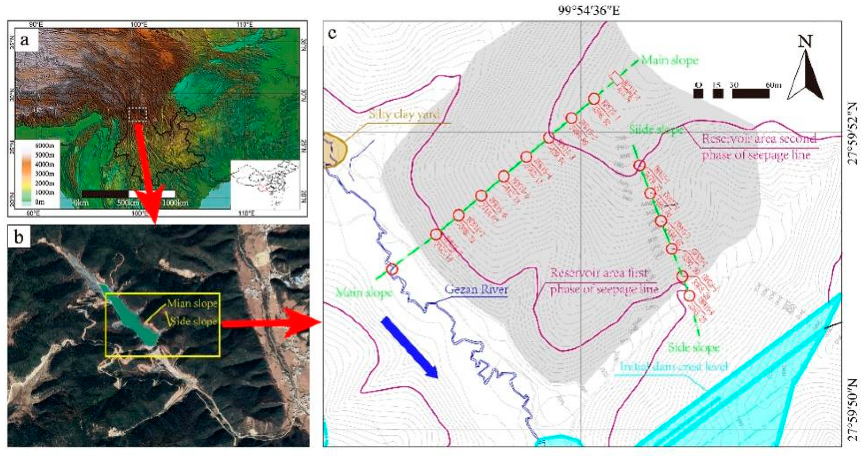
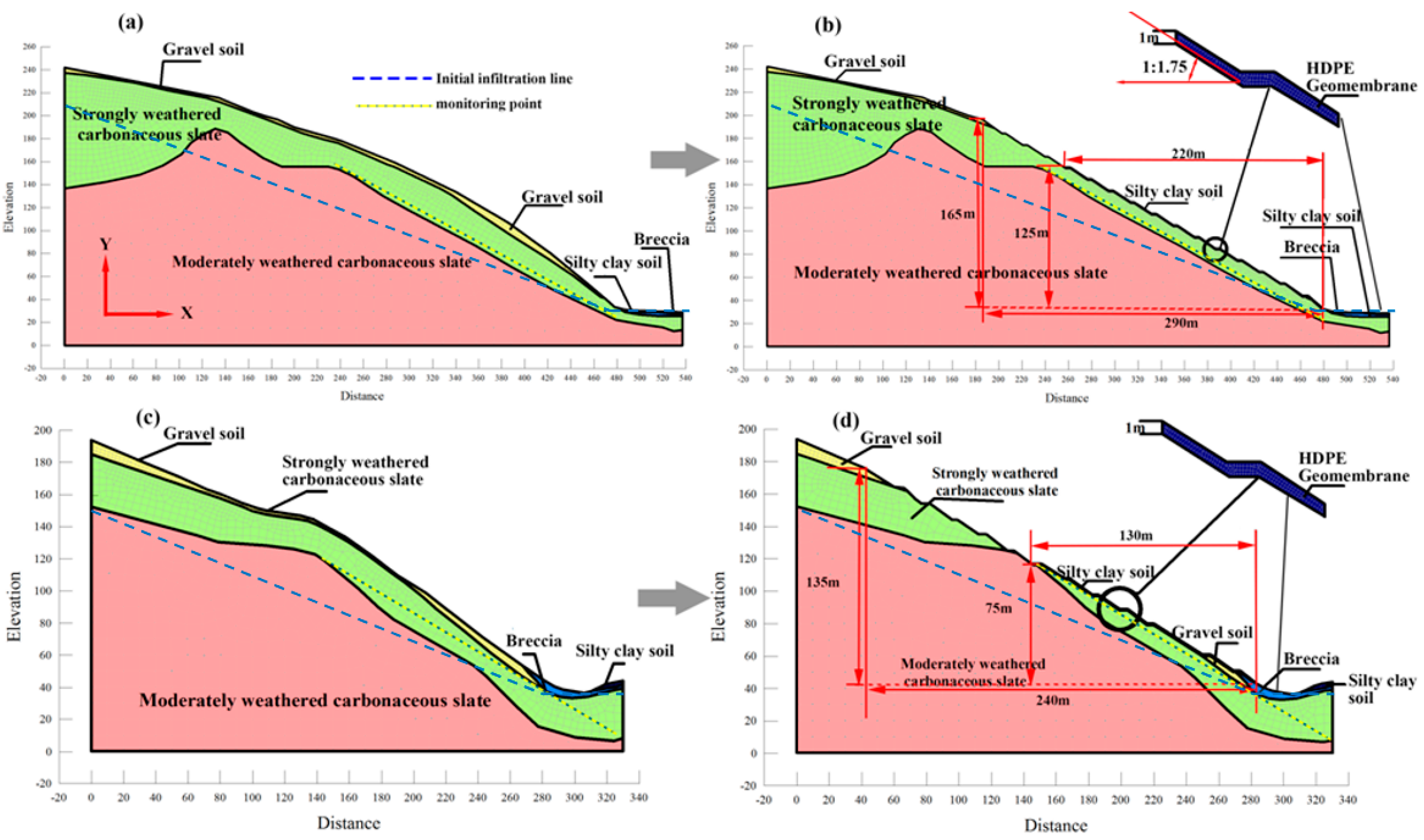
The Pulang copper mine, located in Yunnan Province, China (Figure 1), is one of the largest underground copper mines in the country. The selected bank slopes are near the rockfill dam of its tailings pond, the Yulangpei tailings pond. In the numerical calculation model, the X (538 m) direction of the main slope is perpendicular to the surface runoff, and the Y (242 m) direction runs vertically upwards, as shown in Figure 2a; the X (328 m) direction of the side slope is almost parallel to the surface runoff, and the Y (196 m) direction runs vertically upwards, as shown in Figure 2c. The sizes of the slope and model after GSP remain unchanged. The height of the main slope is about 165 m, and the length is about 290 m (Figure 2b). The height and length of the side slope are roughly 135 and 240 m, respectively (Figure 2d). For the numerical simulation, we set 59 monitoring points on the main slope and 66 monitoring points on the side slope. The slopes were covered by the geomembrane with a thickness of 0.5–2 mm, which has an actual permeability coefficient value of 10–13 cm/s. To simulate the geomembrane, the total volume of seepage flow is constant, according to the equivalent principle of seepage. Therefore, the equivalent permeability coefficient, , and the equivalent thickness, , can be expressed as:
Cen et al. [31] reported that the equivalent thickness 1000 mm (1 m) has the equivalent permeability coefficient of 10–13 cm/s and the optimized numerical simulation effect. The height and length of the geomembrane on the main slope are 125 and 220 m, respectively (Figure 2c), and the corresponding values on the side slope are 75 and 130 m (Figure 2d).
2.3. Calculation Parameters
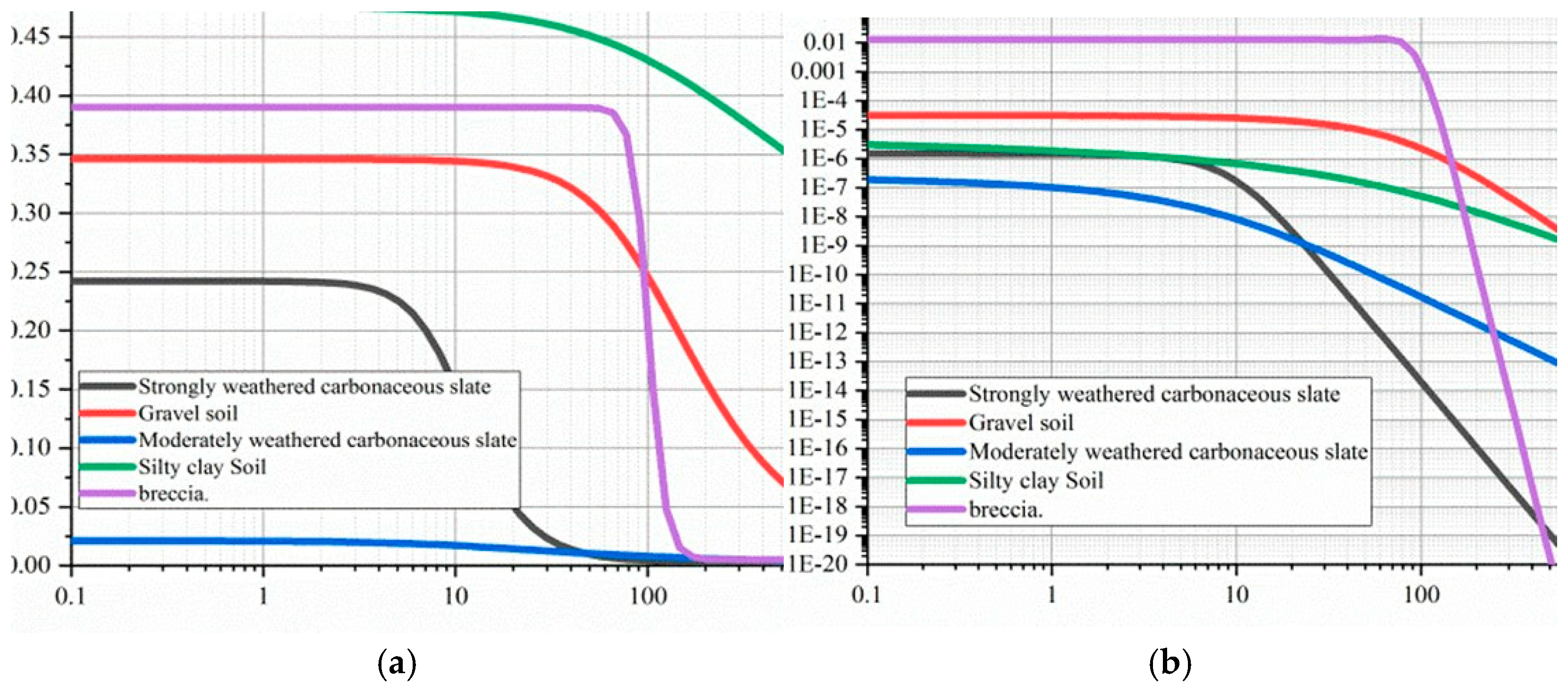
The rock and soil constitutive model follows the Mohr–Coulomb model, and the FS was calculated by the Morgenstern–Price method. Table 1 lists the rock and soil layer parameters of the bank slope, which are from quality surveys and laboratory tests. The parameters of the water retention curve were determined by the Van Genuchten model parameter sensitivity analysis and the literature [32] (Table 2). The relationship (Figure 3) between the volumetric water content, permeability coefficient, and matrix suction in the soil–water characteristic curve was determined by geological survey data and equation derivation.
2.4. Model Boundary Conditions
According to hydrogeological records, the initial water level at the far bank of the main slope is approximately 210 m, and that of the near-shore groundwater head is roughly 30 m. The initial water level at the side slope is fixed, about 150 m. The near-shore end groundwater head is approximately 40 m, allowing the model to seep naturally for 600 days, and therefore the seepage-to-matrix suction is stable. The simulated period is 120 days. The numerical simulation considers three dynamic boundary conditions and their time-varying properties, which are defined as follows:
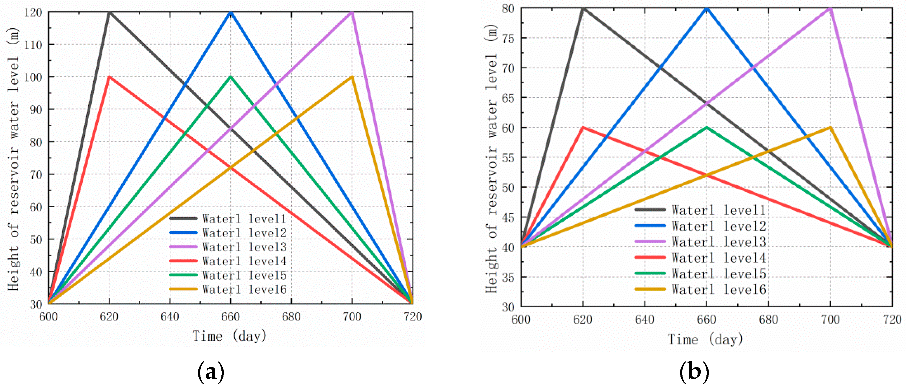
Condition 1: Different reservoir water levels and different rising and falling rates. We assume that the water level has linear change modes (Figure 4): mode 1, fast rising and slow falling (water levels 1 and 4); mode 2, moderate rising and falling (water levels 2 and 5); and mode 3, slow rising and fast falling (water level 3 and 6). There are six cases in each category, as shown in Figure 4.
Condition 2: Rainfall infiltration boundary. We simulate a 5-day consecutive rainfall with nine intensities: 1 mm/h, 3 mm/h, 5 mm/h, 7 mm/h, 9 mm/h, 11 mm/h, 13 mm/h, 15 mm/h, and 17 mm/h. After the rain stops, the stability of the bank slope seepage condition without rainfall for 5 days is simulated.
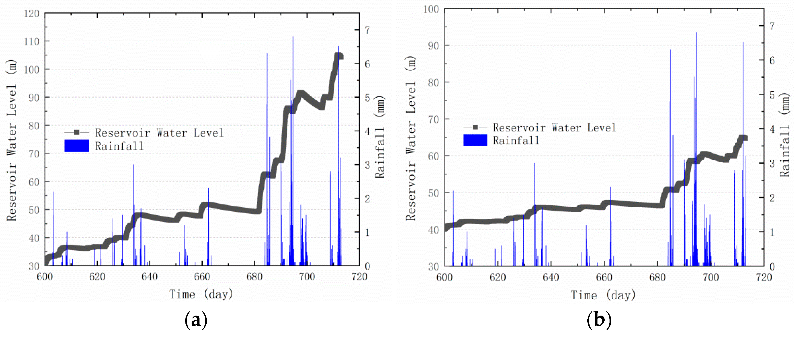
Condition 3: Simulate the coupling influence of real rainfall and reservoir water level on bank slope stability using the real-time rainfall data and reservoir water level from 24:00 on 1 March 2019 to 24:00 on 27 July 2019, as shown in Figure 5.
3. Simulation Analysis
3.1. Simulation Analysis 1
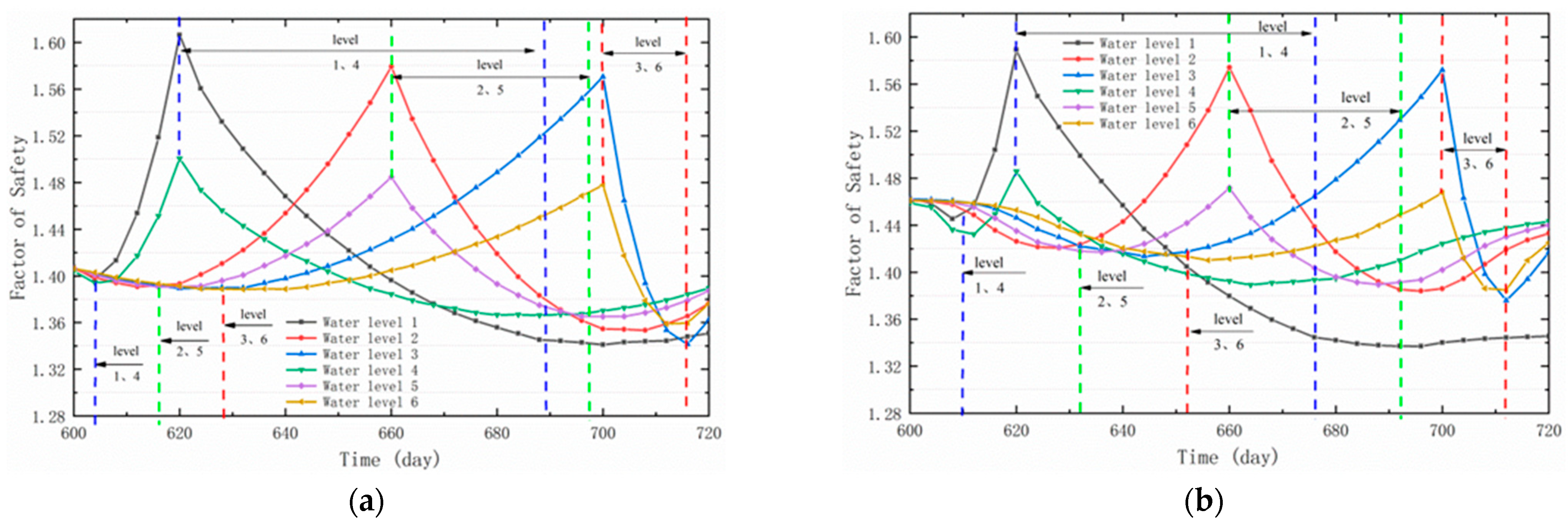
Figure 6 and Figure 7 show the FS of the bank slopes under condition 1. If the water level rises slowly, whether the reservoir water level rises or falls, the valley of the factor of safety (VFS) appears only once. Therefore, there is no peak of the factor of safety (PFS). If the rise is fast, the VFS appears twice, thus a PFS presents. The faster and higher the water level rises, the more a PFS appears.
The bank slope FS change is positively related to the variation of the water level. When the water level rises fast, the FS also increases. This is because the PWP in the slope grows slower than water pressure on the main slope [33], resulting in reverse pressure on the slope foot, which slows the transformation of the slope body from unsaturation to saturation. The negative pressure zone decelerates, resulting in an increase in the bank slope FS. On the other hand, the faster the reservoir water level decreases, the faster the FS decreases. This is because the slope’s groundwater level declines after the reservoir water level, and the PWP decreases slower than the water pressure on the main slope. Consequently, excess PWP and water pressure are generated outside the slope. There is a lag between the FS change and the water level change; that is, the smallest FS does not appear when the water level is the highest but some time later [34]. This lag is most obvious for water level 1 in mode 1, and it is least obvious for water level 6 in mode 3. For the main slope, the VFS appeared the latest in mode 3 (water levels 3 and 6) and the earliest in mode 1 (water levels 1 and 4) (Figure 6).
After GSP, the bank slope stability improves, and the FS changes similarly to that of before GSP. Furthermore, the side slope lag is enhanced, but that of the main slope is weakened. The main slope VFS appears later. The side slope FS is clearly improved, yet that of the main slope is not significantly improved. The main slope PFS decreases, and that of the side slope increases significantly.
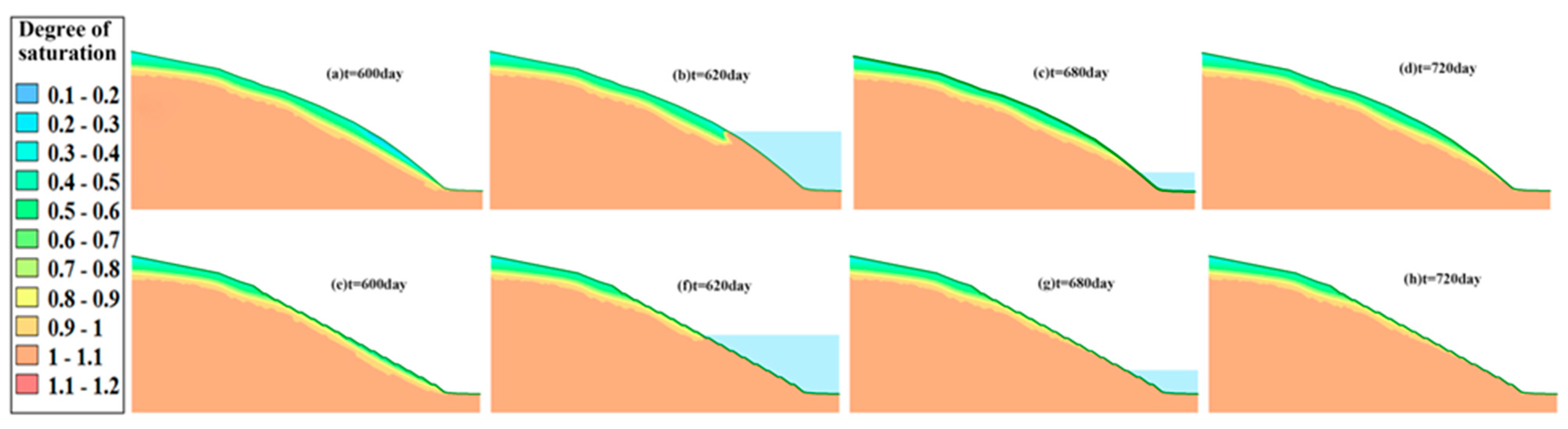
Figure 8 and Figure 9 show the progressive saturation and horizontal displacement of the slope at water level 1. Initially, the saturation above the water level is inversely proportional to the elevation; that is, the further from the water level, the smaller the saturation degree. The initial horizontal displacement is zero. After 20 days of the water level rising, the slope internal saturation degree rises. The water level rises faster than the slope infiltration line, resulting in a concave saturation curve. The soil shear strength is low, and the horizontal displacement is large under the soil–water coupling effect. After 60 days, the water level and infiltration line both drop. As the infiltration line goes down, the slope saturation degree decreases, and the slope seeps outwards, which in turn generates dynamic water pressure and excess PWP. Consequently, the slope’s horizontal displacement is intensified. After another 40 days, the water level drops further. Although the water level at this point has returned to its initial height, the soil saturation degree is higher than its initial state, as it is soaked in water. In such a case, the displacement increases slowly. After grading, the unsaturated area of the slope decreases, and the slope’s saturation and horizontal displacement are more sensitive to water level changes. The horizontal displacement area increases, and the maximum displacement area approaches the slope foot.
3.2. Simulation Analysis 2
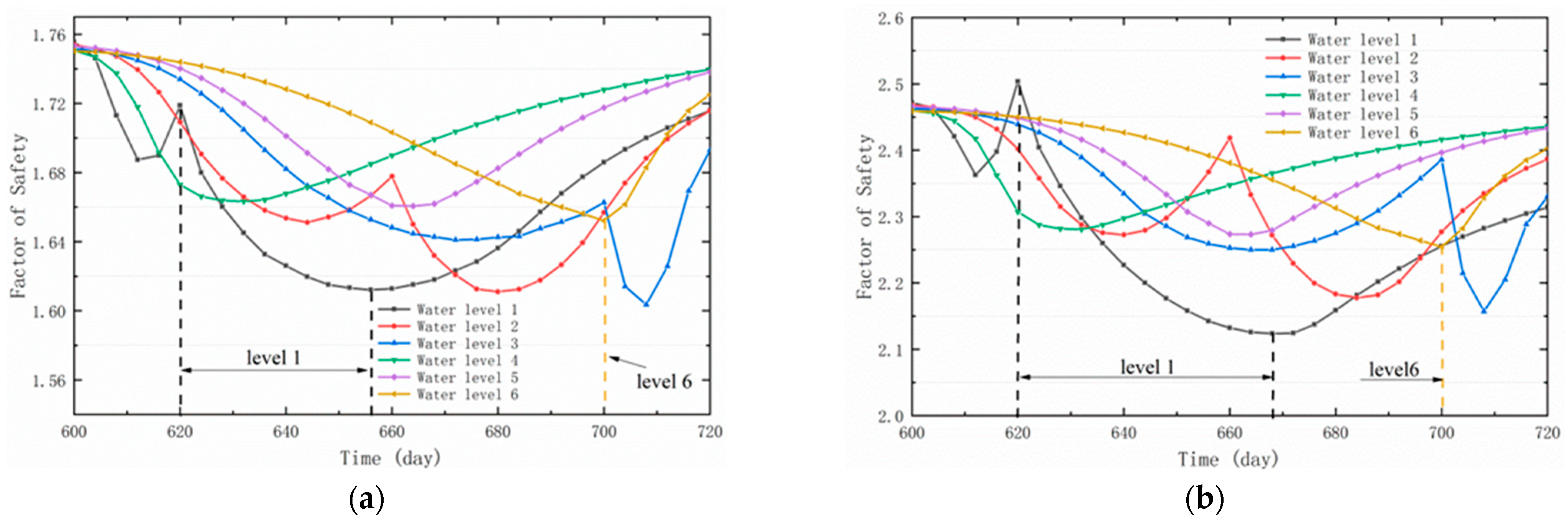
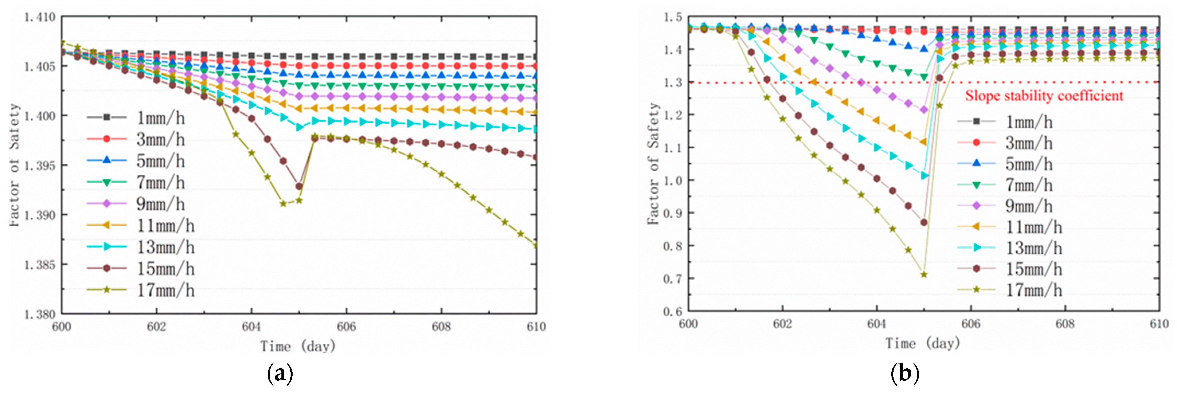
As Figure 10 and Figure 11 show, the stronger the rainfall, the smaller the FS. When the rainfall stops, the FS rebounds. Before GSP, during a heavy rainfall period, the slope FS decreases twice. The first drop occurs during rainfall. After a short and intensive rainfall, a strong outward tilting water pressure is generated inside the slope, which decreases the slope stability [35]. The second drop occurs after the rain stops. As the mine drainage lags behind the rainfall, a large amount of water is stored in the pond. When the rainfall stops, the drainage Increases and the slope continues seeping and produces a strong outward water pressure, decreasing the slope stability.
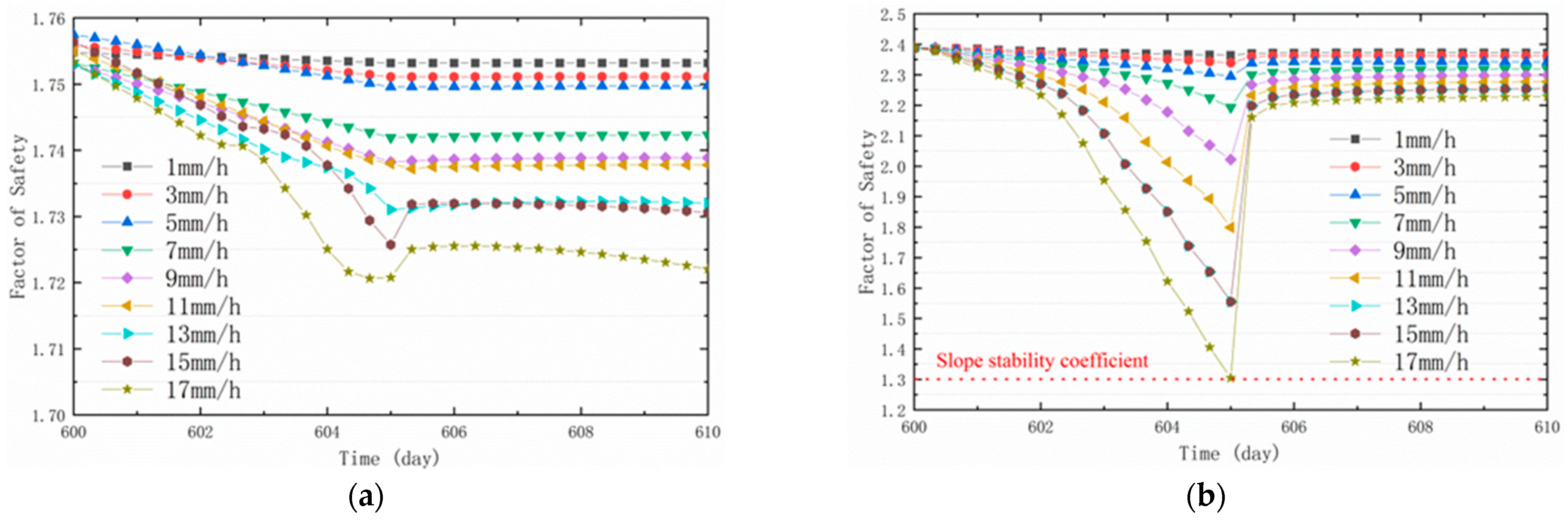
According to the Technical Specification for Construction Slope Engineering (GB50330-2013), the stability coefficient of the bank slope is 1.3, as shown in Figure 10b. After GSP, the initial and final FS of the main slope are enhanced, and the sensitivity to rainfall is also improved. But during rainfall with an intensity greater than 7 mm/h, the FS reduces to smaller than 1.3, indicating that the main slope needs further protection. After GSP, the initial and final FS of the side slopes are significantly improved. If the rainfall intensity is not greater than 9 mm/h, the sensitivity to rainfall is reduced. When the rainfall intensity exceeds 13 mm/h, the FS reduces but remains in a stable state, as shown in Figure 11b. Considering the single-day maximum rainfall intensity in the study area is 8 mm/h, the side slope GSP is safe and reliable.
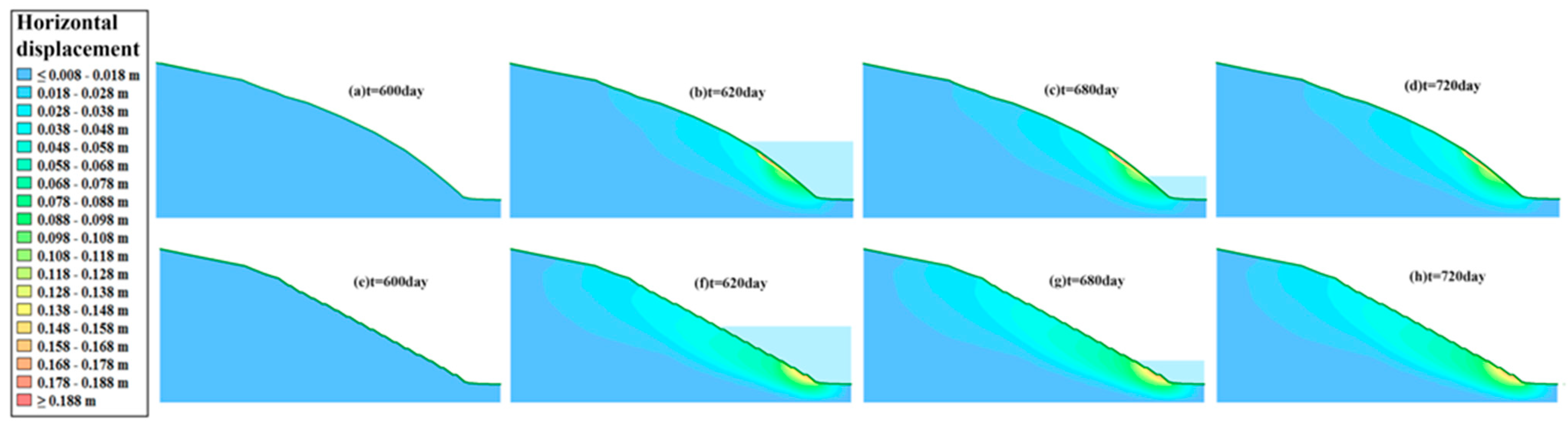
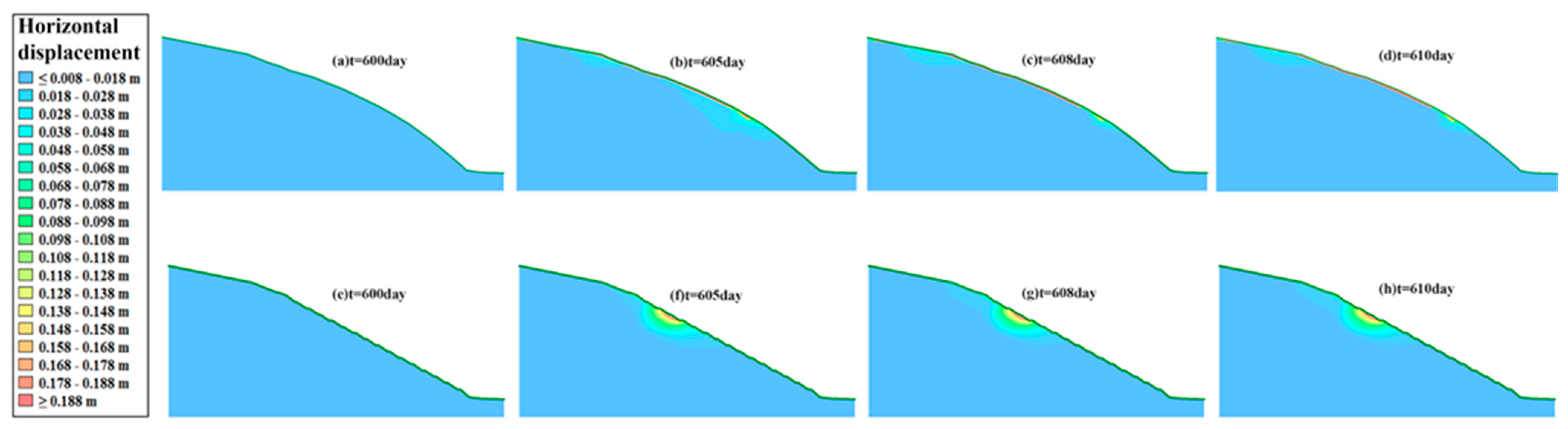
Figure 12 and Figure 13 show the progressive saturation and horizontal displacement of the main slope under the rainfall intensity of 17 mm/h. After a 5-day heavy rainfall, the saturation degree of the slope surface increases sharply, and so does the horizontal displacement. Three days after the rain, the surface water infiltrates into the slope, decreasing the slope surface saturation degree and the horizontal displacement. Five days after the rain, the surface water infiltration continues, increasing both the saturation zone and the horizontal displacement slowly. After GSP, the impervious layer slows the water outflow, and the middle and lower parts of the slope draw close to saturation. The horizontal displacement area instigated by heavy rainfall is increased.
3.3. Simulation Analysis 3
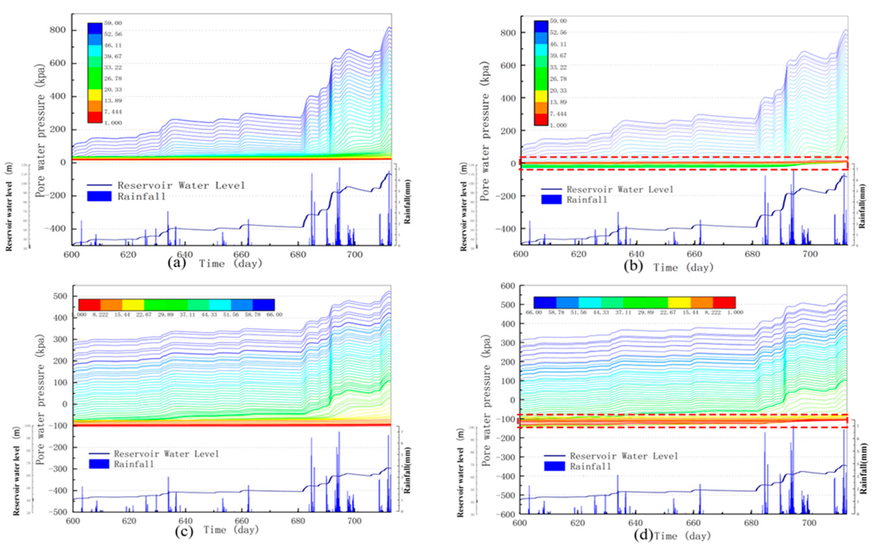
Figure 14 shows the PWP changes in the 59 monitoring points on the main slope and the 66 monitoring points on the side slope. The smaller the monitoring point number, the higher the altitude. For the monitoring points above the highest water level, the PWP is only affected by the changes in the water level. The farther the monitoring point from the highest water level, the smaller the PWP, and it eventually reaches a fixed value. For the monitoring points below the highest reservoir water level, the PWP has a similar variation trend with the reservoir water level. Furthermore, the closer the monitoring point to the slope bottom, the greater the PWP change. After GSP, a negative pressure zone appears in the middle of the main slope, and that in the lower and middle parts of the side slope increases, which is indicated by the red dotted area.
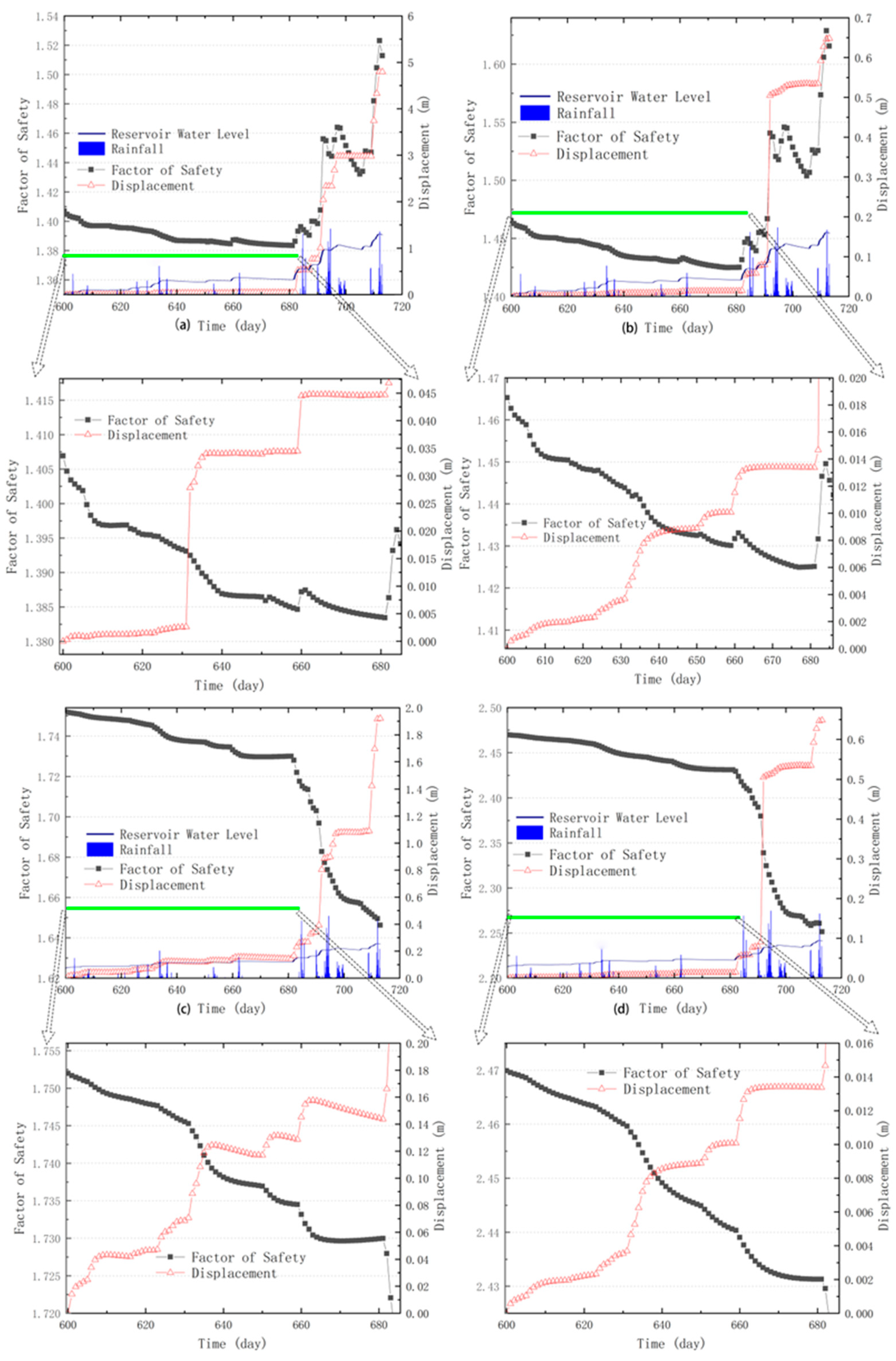
Figure 15a shows the FS and displacement of the main slope from 1 March to 27 July. The overall change trend shows a small decline followed by a sharp rise. This is correlated with increased rainfall intensity, faster water level rise, and occurrence in the rainy season. The displacement is the sum of all monitoring points, which increases steadily. As the rainfall intensity increases and the water level rises, the displacement increases. After GSP, the overall FS increases by about 3%, and the total displacement reduces by about 87%. Figure 15b shows the corresponding values of the side slope. From 1 March to 27 July, the FS is negatively correlated with the change in total displacement. The overall trend shows a slight rise followed by a sharp rise. This is related to the increased rainfall intensity and fast water level rise in the rainy season. After GSP, the overall FS of the side slope increases by approximately 41%, and the total displacement decreases by about 66%. When the rainfall intensity is greater than 4 mm/h, the total displacement increases significantly.
4. Conclusions
In this paper, the slope stability of the Yulangpei tailings pond is investigated considering grading and seepage prevention. Under three common hydraulic boundary conditions, SEEP/W is applied to analyze the finite element unsaturated seepage on the bank slope, and the SLOPE/W software implements the Morgenstern–Price method to analyze the bank slope stability by solving for the FS. Finally, the SIGMA/W software is used to investigate the horizontal displacement, based on the soil–water coupling theory. The following conclusions can be drawn:
- Under the combined effects of two reservoir water levels and three different rising and falling speeds, the change in the bank slope FS occurs later than the water level change. Such a lag expands as the water level rises faster and higher, and slower water level declines occur. Meanwhile, the PFS of the three water level modes increases when the water level rises faster and higher.
- When there is rainfall, the FS decreases faster with higher rainfall intensity. In addition, the FS increases after the rainfall stops. The initial stability of the bank slope under different conditions was improved after the GSP measures, but the main slope was more sensitive to the changes in rainfall and water level.
- Under the coupling effects of real rainfall infiltration and reservoir water fluctuation from 1 to 27 July 2019, the PWP changed. The farther the monitoring point from the highest water level, the lower the PWP, and vice versa. The displacement is positively correlated with the rainfall intensity and concentration.
- Simulations for all three conditions indicate that GSP improves the FS of the slopes with no significant improvement to the main slopes but a significant improvement to their total displacement.
Author Contributions
Conceptualization, Y.F. and F.Y.; formal analysis, L.W. and T.L.; writing—original draft, Y.F. and F.Y.; and writing—review and editing, L.W., G.L. and T.L. All authors have read and agreed to the published version of the manuscript.
Funding
This work was financially supported by the National Natural Science Foundation of China under Grant No. 41974148 and No. 52004327; the Hunan Provincial Key Research and Development Program, Grant No. 2020SK2135; the Natural Resources Research Project of Hunan Province, Grant No. 2021-15; and the Science and Technology Project of Hunan Provincial Department of Transportation, Grant No. 202012.
Data Availability Statement
The source data can be obtained from the article.
Conflicts of Interest
The authors declare no conflict of interest.
References
- Fourniadis, I.G.; Liu, J.G.; Mason, P. Regional assessment of landslide impact in the Three Gorges area, China, using ASTER data: Wushan-Zigui. Landslides 2007, 4, 267–278. [Google Scholar] [CrossRef]
- Cojean, R.; Caï, Y. Analysis and Modeling of Slope Stability in the Three-Gorges Dam Reservoir (China)—The Case of Huangtupo Landslide. J. Mt. Sci.-Engl. 2011, 8, 166–175. [Google Scholar] [CrossRef]
- Acharya, K.P.; Bhandary, N.P.; Dahal, R.K.; Yatabe, R. Numerical analysis on influence of principal parameters of topography on hillslope instability in a small catchment. Environ. Earth Sci. 2015, 73, 5643–5656. [Google Scholar] [CrossRef]
- Reid, I.; Parkinson, R.J. The wetting and drying of a grazed and ungrazed clay soil. Eur. J. Soil Sci. 1984, 35, 607–614. [Google Scholar] [CrossRef]
- Take, W.A.; Beddoe, R.A.; Davoodi-Bilesavar, R.; Phillips, R. Effect of antecedent groundwater conditions on the triggering of static liquefaction landslides. Landslides 2015, 12, 469–479. [Google Scholar] [CrossRef]
- Pender, M.J.; Orense, R.P.; Wotherspoon, L.M.; Storie, L.B. Effect of permeability on the cyclic generation and dissipation of pore pressures in saturated gravel layers. Géotechnique 2016, 66, 313–322. [Google Scholar] [CrossRef]
- Wei, Z.; Yin, G.; Wang, J.; Wan, L.; Jin, L. Stability analysis and supporting system design of a high-steep cut soil slope on an ancient landslide during highway construction of Tehran–Chalus. Environ. Earth Sci. 2012, 67, 1651–1662. [Google Scholar] [CrossRef]
- Wen, B.-P.; He, L. Influence of lixiviation by irrigation water on residual shear strength of weathered red mudstone in Northwest China: Implication for its role in landslides’ reactivation. Eng. Geol. 2012, 151, 56–63. [Google Scholar] [CrossRef]
- Chen, J.D.; Ge, X.R.; Song, D.Q.; Cai, J. Deformation and mechanical characteristics of bedding rock slope in tunnel excavation. J. Water Resour. Archit. Eng. 2018, 16, 149–154. (In Chinese) [Google Scholar]
- Ran, T.; Liu, D.A.; Mei, S.H.; Wang, W.; Tan, L. Intelligent feedback analysis on a deep excavation for the gravity anchorage foundation of a super suspension bridge. Chin. J. Rock Mech. Eng. 2019, 38, 2898–2912. (In Chinese) [Google Scholar]
- Singh, J.; Banka, H.; Verma, A. Analysis of slope stability and detection of critical failure surface using gravitational search algorithm. In Proceedings of the 2018 4th International Conference on Recent Advances in Information Technology (RAIT) 2018, Dhanbad, India, 15–17 March 2018; pp. 1–6. [Google Scholar]
- Kang, Z.J.; Tan, Y.; Deng, G.; Bin, W. Impact of Soil Reinforcement in Passive Zone on the Deformation Behaviors of Deep Excavation. J. Yangtze River Sci. Res. Inst. 2017, 34, 119–123. [Google Scholar]
- Zhou, Z.; Wang, X.-Q.; Wei, Y.-F.; Shen, J.-H.; Shen, M. Simulation study of the void space gas effect on slope instability triggered by an earthquake. J. Mt. Sci. 2019, 16, 1300–1317. [Google Scholar] [CrossRef]
- Javdanian, H.; Pradhan, B. Assessment of earthquake-induced slope deformation of earth dams using soft computing techniques. Landslides 2018, 16, 91–103. [Google Scholar] [CrossRef]
- Gomberg, J. Cascadia Onshore-Offshore Site-Response, Submarine Sediment Mobilization, and Earthquake Recurrence. J. Geophys. Res. Solid Earth 2018, 123, 1381–1404. (In Chinese) [Google Scholar] [CrossRef]
- Tang, H.; Hu, X.; Xu, C.; Li, C.; Yong, R.; Wang, L. A novel approach for determining landslide pushing force based on landslide-pile interactions. Eng. Geol. 2014, 182, 15–24. [Google Scholar] [CrossRef]
- VanWoert, N.D.; Rowe, D.B.; Andresen, J.A.; Rugh, C.L.; Fernandez, R.T.; Xiao, L. Green Roof Stormwater Retention: Effects of Roof Surface, Slope, and Media Depth. J. Environ. Qual. 2005, 34, 1036–1044. [Google Scholar] [CrossRef]
- Zhuang, X.; Wang, W.; Ma, Y.; Huang, X.; Lei, T. Spatial distribution of sheet flow velocity along slope under simulated rainfall conditions. Geoderma 2018, 321, 1–7. [Google Scholar] [CrossRef]
- Zhao, L.; Hou, R.; Wu, F.; Keesstra, S. Effect of soil surface roughness on infiltration water, ponding and runoff on tilled soils under rainfall simulation experiments. Soil Tillage Res. 2018, 179, 47–53. [Google Scholar] [CrossRef]
- Fu, X.T. Characteristics of flow pattern and sediment transport processes on loessal soil slope in western Shanxi Province. J. Hydraul. Eng. 2017, 48, 738–747. [Google Scholar]
- Fan, H.M.; Huang, D.H.; Zhou, L.L.; Jin, L. Effects of Seasonal Freeze-thaw Action on Phosphorus Loss of Slope in Black Soil. J. Soil Water Conserv. 2014, 28, 151–152. [Google Scholar]
- Cheng, Y.T.; Li, P.; Xu, G.C.; Li, G.; Zhanbin, W.T. Effect of soil erodibility on nitrogen and phosphorus loss under condition of freeze-thaw. Trans. Chin. Soc. Agric. Eng. 2017, 33, 141–149. [Google Scholar]
- Mandal, A.K.; Li, X.; Shrestha, R. Influence of Water Level Rise on the Bank of Reservoir on Slope Stability: A Case Study of Dagangshan Hydropower Project. Geotech. Geol. Eng. 2019, 37, 5187–5198. [Google Scholar] [CrossRef]
- Sun, G.; Zheng, H.; Tang, H.; Dai, F. Huangtupo landslide stability under water level fluctuations of the Three Gorges reservoir. Landslides 2015, 13, 1167–1179. [Google Scholar] [CrossRef]
- Wei, J.; Deng, J.; Tham, L.; Lee, C.F. Unsaturated seepage analysis for a reservoir landslide during impounding. In Landslides and Engineered Slopes. From the Past to the Future; CRC Press: Boca Raton, FL, USA, 2008; pp. 999–1004. [Google Scholar]
- Xiong, Y.; Bao, X.; Ye, B.; Zhang, F. Soil–water–air fully coupling finite element analysis of slope failure in unsaturated ground. Soils Found. 2014, 54, 377–395. [Google Scholar] [CrossRef]
- Kitamura, R.; Sako, K. Contribution of “Soils and Foundations” to Studies on Rainfall-Induced Slope Failure. Soils Found. 2010, 50, 955–964. [Google Scholar] [CrossRef]
- Lu, N.; Godt, J. Infinite Slope Stability under Steady Unsaturated Seepage Conditions. Water Resour. Res. 2008, 44, 63–75. [Google Scholar] [CrossRef]
- GEO-SLOPE International Ltd. Seepage Modeling with SEEP/W 2007; GEO-SLOPE International Ltd.: Calgary, AB, Canada, 2010; pp. 1–207. [Google Scholar]
- Genuchten, V.M. A Closed-form Equation for Predicting the Hydraulic Conductivity of Unsaturated Soils. Soil Sci. Soc. Am. J. 1980, 44, 892–898. [Google Scholar] [CrossRef]
- Cen, W.J.; Wang, M.; Yang, Z.X. Partial saturated seepage properties of(composite) geomembrane earthrock dams. Adv. Sci. Technol. Water Resour. 2012, 32, 6–9. (In Chinese) [Google Scholar]
- Chen, Y.-F.; Yu, H.; Ma, H.-Z.; Li, X.; Hu, R.; Yang, Z. Inverse modeling of saturated-unsaturated flow in site-scale fractured rocks using the continuum approach: A case study at Baihetan dam site, Southwest China. J. Hydrol. 2020, 584, 124693. [Google Scholar] [CrossRef]
- Wu, Y.; Miao, F.; Li, L.; Xie, Y.; Chang, B. Time-varying reliability analysis of Huangtupo Riverside No.2 Landslide in the Three Gorges Reservoir based on water-soil coupling. Eng. Geol. 2017, 226, 267–276. [Google Scholar] [CrossRef]
- Jiao, Y.-Y.; Zhang, H.-Q.; Tang, H.-M.; Zhang, X.-L.; Adoko, A.C.; Tian, H.-N. Simulating the process of reservoir-impoundment-induced landslide using the extended DDA method. Eng. Geol. 2014, 182, 37–48. [Google Scholar] [CrossRef]
- Zhang, D.; Jian, W.B.; Ye, Q.; Lin, W. A time-varying analytic model of tailings slope and its application. Yantu Lixue/Rock Soil Mech. 2014, 35, 835–840. [Google Scholar] [CrossRef]
Figure 1.
(a) Location of the study site in the northwestern Yunnan Province, China. (b) Google Earth image of the study site. (c) Topographical map of the bank slopes near the dam.
Figure 1.
(a) Location of the study site in the northwestern Yunnan Province, China. (b) Google Earth image of the study site. (c) Topographical map of the bank slopes near the dam.

Figure 2.
The numerical simulation models of the slopes. (a) Grid model of the main slope before GSP. (b) Grid model of the main slope after GSP. (c) Grid model of the side slope before GSP. (d) Grid model of the side slope after GSP.
Figure 2.
The numerical simulation models of the slopes. (a) Grid model of the main slope before GSP. (b) Grid model of the main slope after GSP. (c) Grid model of the side slope before GSP. (d) Grid model of the side slope after GSP.

Figure 3.
Water retention (a) and hydraulic conductivity (b) curves for different slope layers.

Figure 4.
Water level changes in the (a) main and (b) side slopes.

Figure 5.
Water level changes and rainfall of (a) main slope and (b) side slope.

Figure 6.
The FS of the main slope under different reservoir water level modes (a) before and (b) after GSP.
Figure 6.
The FS of the main slope under different reservoir water level modes (a) before and (b) after GSP.

Figure 7.
The side slope FS under different reservoir water level modes (a) before and (b) after GSP.
Figure 7.
The side slope FS under different reservoir water level modes (a) before and (b) after GSP.

Figure 8.
Variation of the saturation of the main slope (a–d) before GSP and (e–h) after GSP.

Figure 9.
Variation of the horizontal displacement of the main slope (a–d) before GSP and (e–h) after GSP.
Figure 9.
Variation of the horizontal displacement of the main slope (a–d) before GSP and (e–h) after GSP.

Figure 10.
Variation of the main slope FS under different reservoir water level modes (a) before and (b) after GSP.
Figure 10.
Variation of the main slope FS under different reservoir water level modes (a) before and (b) after GSP.

Figure 11.
Variation of the FS of the side slope under different reservoir water level modes (a) before GSP and (b) after GSP.
Figure 11.
Variation of the FS of the side slope under different reservoir water level modes (a) before GSP and (b) after GSP.

Figure 12.
Saturation of the main slope under a rainfall intensity of 17 mm/h (a–d) before and (e–h) after GSP.
Figure 12.
Saturation of the main slope under a rainfall intensity of 17 mm/h (a–d) before and (e–h) after GSP.

Figure 13.
Horizontal displacement of the main slope under a rainfall intensity of 17 mm/h (a–d) before and (e–h) after GSP.
Figure 13.
Horizontal displacement of the main slope under a rainfall intensity of 17 mm/h (a–d) before and (e–h) after GSP.

Figure 14.
The PWP of (a) the 59 monitoring points of the main slope before GSP. (b) the 59 monitoring points of the main slope after GSP, (c) the 66 monitoring points on the side slope before GSP and (d) at the 66 monitoring points on the side slope after GSP.
Figure 14.
The PWP of (a) the 59 monitoring points of the main slope before GSP. (b) the 59 monitoring points of the main slope after GSP, (c) the 66 monitoring points on the side slope before GSP and (d) at the 66 monitoring points on the side slope after GSP.

Figure 15.
Variation of the FS and displacement under condition 3 for (a) main slope before GSP, (b) main slope after GSP, (c) side slope before GSP, and (d) side slope after GSP.
Figure 15.
Variation of the FS and displacement under condition 3 for (a) main slope before GSP, (b) main slope after GSP, (c) side slope before GSP, and (d) side slope after GSP.


Table 1.
Parameters of slope layers.
| Materials | Elastic Modulus (MPa) | Poisson Ratio | Unit Weight (kN/m3) | Cohesion (kPa) | Friction Angle (°) |
|---|---|---|---|---|---|
| Gravel soil | 261.6 | 0.4 | 20.5 | 15 | 32 |
| Strongly weathered carbonaceous slate | 2644.9 | 0.38 | 22.4 | 93.6 | 33.3 |
| Moderately weathered carbonaceous slate | 5561 | 0.35 | 26.5 | 120 | 35 |
| Silty clay soil | 179.8 | 0.42 | 18.5 | 35 | 15 |
| Breccia | 222.7 | 0.42 | 20 | 15 | 30 |
Table 2.
Parameters of the water retention curve of slope layers.
| Materials | SWCC Parameters | Hydraulic Conduction Coefficient | ||||
|---|---|---|---|---|---|---|
| a/kPa | m | n | θs | θr | kx (m/s) | |
| Gravel soil | 100 | 0.5 | 2 | 0.346 | 0.005 | 3.14 × 10⁻³ |
| Strongly weathered carbonaceous slate | 10 | 0.31 | 1.45 | 0.242 | 0.001 | 8.08 × 10⁻⁵ |
| Moderately weathered carbonaceous slate | 10 | 0.31 | 1.45 | 0.021 | 0.001 | 2.47 × 10⁻⁶ |
| Silty clay soil | 100 | 0.145 | 1.17 | 0.476 | 0.001 | 6.51 × 10⁻⁶ |
| Breccia | 100 | 0.5 | 2 | 0.39 | 0.005 | 1.28 × 10⁻² |
| HDPE geomembrane | 1 × 10⁻¹⁵ |
Disclaimer/Publisher’s Note: The statements, opinions and data contained in all publications are solely those of the individual author(s) and contributor(s) and not of MDPI and/or the editor(s). MDPI and/or the editor(s) disclaim responsibility for any injury to people or property resulting from any ideas, methods, instructions or products referred to in the content. |
© 2023 by the authors. Licensee MDPI, Basel, Switzerland. This article is an open access article distributed under the terms and conditions of the Creative Commons Attribution (CC BY) license (https://creativecommons.org/licenses/by/4.0/).
Share and Cite
MDPI and ACS Style
Feng, Y.; Yan, F.; Wu, L.; Lu, G.; Liu, T. Numerical Analyses of Slope Stability Considering Grading and Seepage Prevention. Water 2023, 15, 1745. https://doi.org/10.3390/w15091745
AMA Style
Feng Y, Yan F, Wu L, Lu G, Liu T. Numerical Analyses of Slope Stability Considering Grading and Seepage Prevention. Water. 2023; 15(9):1745. https://doi.org/10.3390/w15091745
Chicago/Turabian StyleFeng, Yuting, Fuyu Yan, Lianrong Wu, Guangyin Lu, and Taoying Liu. 2023. "Numerical Analyses of Slope Stability Considering Grading and Seepage Prevention" Water 15, no. 9: 1745. https://doi.org/10.3390/w15091745
Note that from the first issue of 2016, this journal uses article numbers instead of page numbers. See further details here.