
Application of Artificial Neural Networks for Predicting Small Urban-Reservoir Volumes: The Case of Torregrotta Town (Italy)

Department of Engineering, University of Messina, 98166 Messina, Italy
*
Author to whom correspondence should be addressed.
Water 2023, 15(9), 1747; https://doi.org/10.3390/w15091747
Submission received: 29 March 2023
/
Revised: 26 April 2023
/
Accepted: 28 April 2023
/
Published: 1 May 2023
(This article belongs to the Special Issue Application of Artificial Intelligence in Hydraulic Engineering)
Abstract
:In the hydraulic construction field, approximated formulations have been widely used for calculating tank volumes. Identifying the proper water reservoir volumes is of crucial importance in order to not only satisfy water demand but also to avoid unnecessary waste in the construction phase. In this perspective, the planning and management of small reservoirs may have a positive impact on their spatial distribution and storage capacities. The purpose of this study is, therefore, to suggest an alternative approach to estimate the optimal volume of small urban reservoirs. In particular, an artificial neural network (ANN) is proposed to predict future water consumption as a function of certain environmental parameters, such as rainy days, temperature and the number of inhabitants. As the water demand is strongly influenced by such quantities, their future trend is recovered by means of the Copernicus Climate Change Service (C3S) over the next 10 years. Finally, based on ANN prediction of the future consumption requirements, the continuity equation applied to tanks was resolved through integral-discretization obtaining the time-series volume variation and the total number of crisis events.
1. Introduction
Among the topics of sustainable development, water resources and the services they provide are indicated as the driving forces to create social, economic and financial equity and, in turn, contribute to alleviate land exploitation and poverty and to improve health, food and energy production and environmental preservation [1]. In this perspective, reservoirs assume a key role in water management due to their functions in water supply, irrigation and soil conservation; industrial and hydropower use; as well as flood protection and control [2].
Focusing on municipal water use, in the literature, there are several examples of tank volume calculations that estimate the capacity as the sum of multiple rates [3]. In particular, water supply systems have been traditionally designed according to deterministic approaches, specifying tank components for balancing incoming and outcoming flow, fire protection and emergency storage due to potential interruptions of the supply lines [4]. Most of the available formulations for water storage determination depend on the inhabitant number and are based on the hypothesis that each user consumes a fixed water quantity [5].
Water demand, on the other hand, is highly variable, and it is influenced by a large number of factors due to its dependence on several environmental parameters [6], including weather conditions and anthropogenic aspects [7,8,9]. For example, [10] observed that rainfall, roof area, number of residents as well as rainwater demand strongly influence tank sizing. It must be considered that, in order to estimate water demand, time series affected by both weekly and yearly periodicity can be employed [7]. The annual periodicity strongly relates to weather conditions, while the weekly or seasonal trend can be related to the fluctuation of non-resident inhabitants.
Empirical approaches have been frequently adopted to determine the reliability of water resources for a municipal water supply system in the light of future demand needs [11]. As well, stochastic methods have been successfully applied to describe the real-time dynamics in reservoirs [12] or for analyzing the reliability of municipal storage tanks [4]. Among such approaches, Monte Carlo methods have been frequently used to tackle uncertainty analysis in complex environmental systems.
As indicated by [13], these approaches fully respect the physical constraints, evaluating the operation constraints in probabilistic terms and allowing the distribution functions and statistics to be derived through Monte Carlo simulation. Recently, ref. [14] used a Monte Carlo method to estimate the uncertainty of average monthly streamflow discharge from a hydrological model in the reservoir system, but other applications can also be found in sewage systems with optimal pumping requirements [15].
On the other hand, conceptual or physically-based models have been adopted to determine tank volume and its management rules [16]. For example, ref. [17] developed a mathematical model for assessing operative policies for a reservoir system based on a computationally efficient optimization procedure. Modern advancements in computer technology have led to the development of complex simulation models widely used in professional practice (i.e., HEC-ResSim [18,19], the WEAP model [20,21] and the CalSim model [22,23]).
Such models present mathematical bases for estimating tank outflow and storage combined with empirical operation rule curves based on historical hydrological data, which are particularly effective in water management tasks [24]. However, such approaches require professional expertise and high-resolution data about watershed characteristics and environmental parameters, and these can fail when multiple complex factors or nonlinear problems have to be faced.
Recently, the advancement in artificial intelligence (AI) has led data-driven models to become popular tools for defining reservoir operations [25]. AI models, compared to physically based ones, show significantly faster response, great learning abilities and better performance in modeling complex formulations. Among AI and machine-learning algorithms, artificial neural networks (ANNs) are black-box models, widely used in several research areas, including hydrology and hydraulics, and they are applied when it is difficult to identify the functional relationships between variables [26].
In the literature, several works deal with the application of ANN to water consumption [27,28,29]. For instance, Walker et al. performed an interesting study using ANN training for investigating hot water consumption [30]. Ref. [31] applied recurrent neural networks to simulate the operation of three multi-purpose reservoirs under different flow regimes—in particular, under extreme floods and droughts—demonstrating their potential applicability in practical water management, particularly for real-time reservoir operations.
Ref. [32] predicted reservoir volumes using several AI techniques, i.e., (ANN), support vector regression (SVR) and long short-term memory (LSTM), applying the aforementioned algorithms to two reservoirs in Turkey and obtaining better performances with ANN and LSTM models. In addition, ref. [33] compared different soft computing models with conventional approaches to forecast water consumption using real datasets from South Africa to understand the effects of the input parameters on the water consumption forecast.
From what is mentioned above, it is clear that the use of ANNs requires a considerable amount of data both for training and testing. The present study reports the application of an ANN to a case study in order to estimate the future consumption of the small town of Torregrotta in Sicily (Italy), using measurements of the consumption flow rate conducted with the aid of a non-remote flow meter. The main aim of this work was to recover the optimal volume to be assigned to small urban reservoirs in order to satisfy future water demand in such a way to also positively impact both the tank spatial distribution and storage capacities.
The paper is organized as follows. In Section 2, we demonstrate that the consumption trends depend on the rain events and temperature tendencies. These occurrences are related to the high percentage of houses with gardens. Due to the lack of a clear trend between the environmental parameters and the water consumption, we deemed it necessary to use an ANN. We obtain the measured water volume as output and the temperature, the number of rainy days and population as input. After the development of the ANN, as shown in Section 3.1, the neural network training leads to a good correlation for the testing and training data.
The future trends of the environmental parameters are successively recovered through the Copernicus platform, re-sampling data from a yearly scale to a monthly scale by means of an adaptive function. The obtained values are used as input for training the ANN in order to obtain future consumption volumes. To predict the tank volume, the monthly volumes are re-sampled at an hourly scale, by means of the already mentioned adaptive model functions. Finally, through the resolution of the continuity equation applied to the tank, imposing a value for the maximum volume, it is possible to obtain the future volume trend and the total number of hours of crisis. The paper ends with some conclusive remarks.
2. Materials and Methods
2.1. Study Area
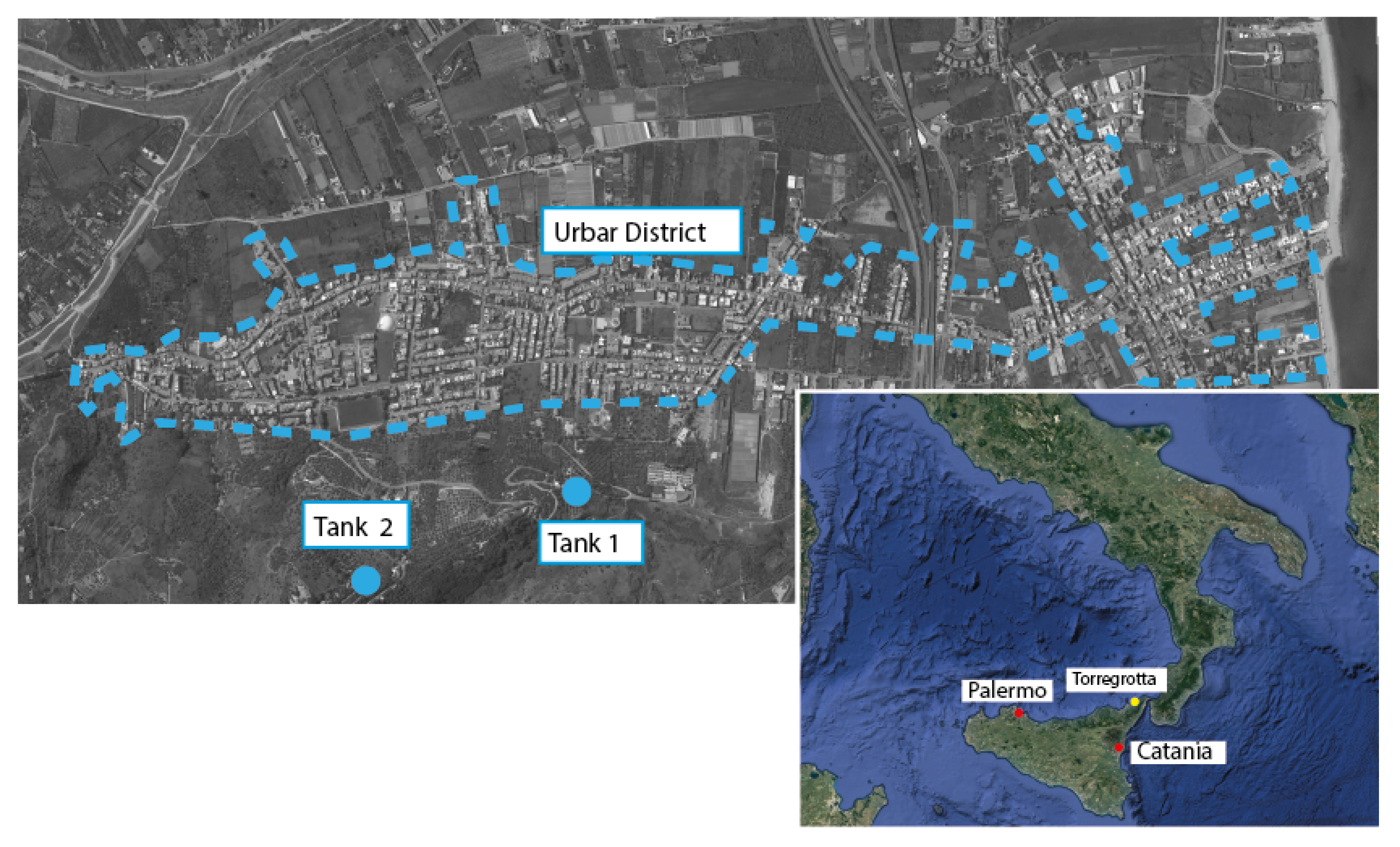
The considered case study refers to the town of Torregrotta (Messina, Italy) (Figure 1). Here, in the past, several crisis events led to shortages in the water supply. The hydraulic network is served by to two tanks, as identified in Figure 1, where -1 and -2 are connected in series. After several interventions performed on the pipe network, it was observed that the problem persisted, meaning that the volume of the tanks was no longer adequate.
2.2. Description of the Existing Reservoirs and Water Network
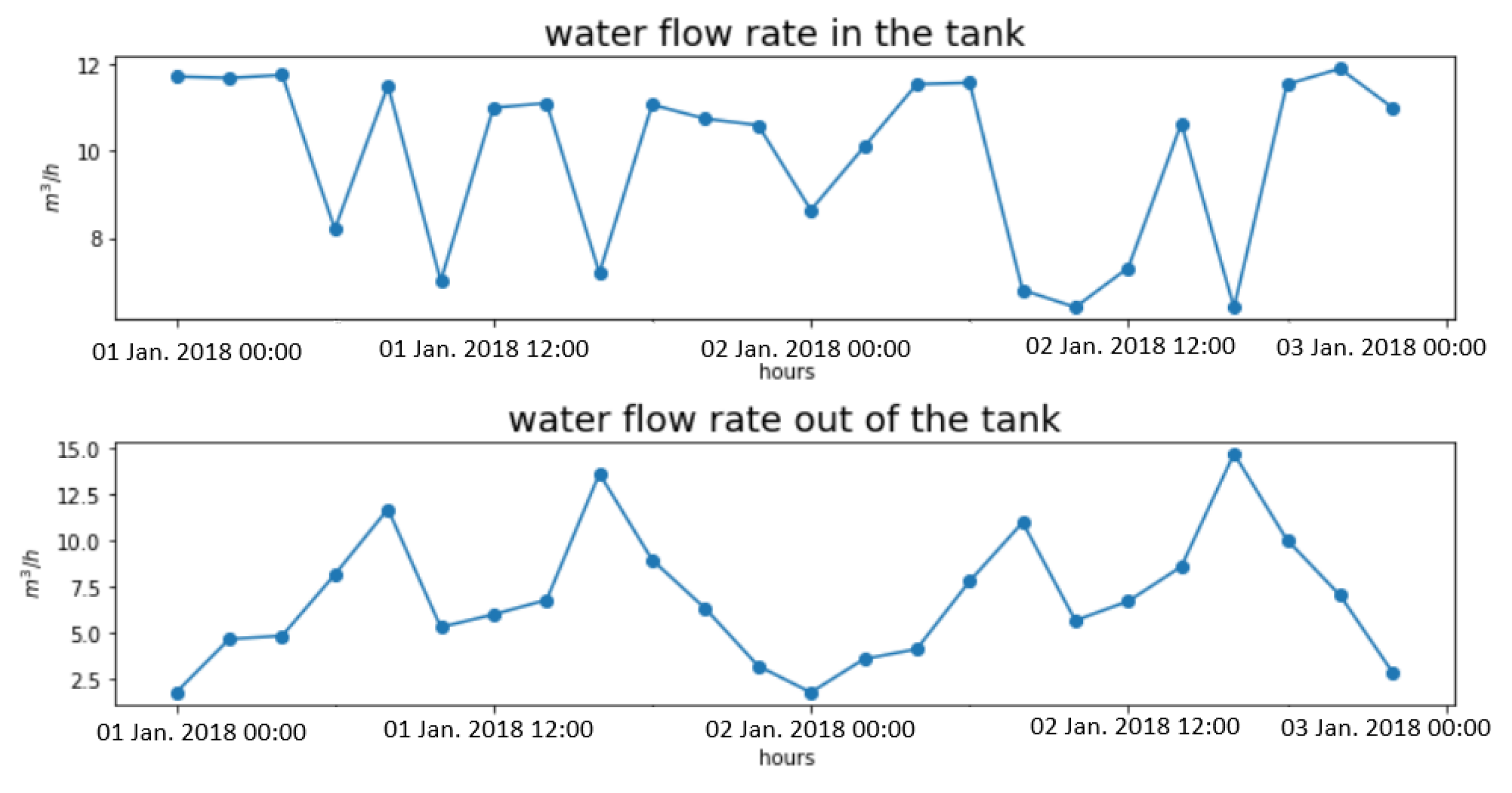
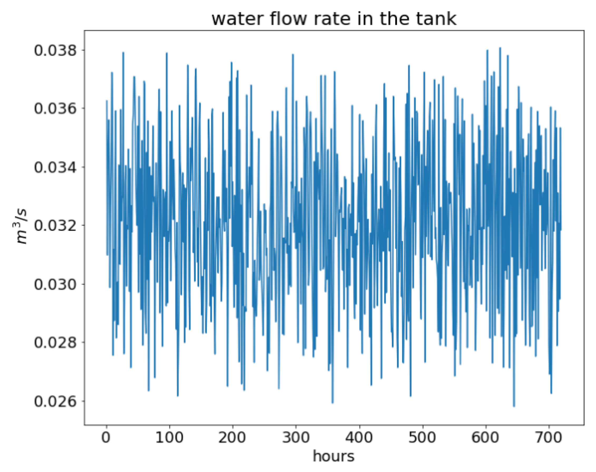
The two above-mentioned reservoirs serve the urban district shown in Figure 1. Both have the same piezometric head of m above sea level. -1 was built between 1972 and 1980 [34], while -2 was built later, in the 2000s, to cope with the increasing compensation crises. The total volume of both tanks equals 1750 m3, with -1 contributing 1000 m3 [34]. The water level inside the tanks can reach a maximum depth of m. The tanks assume a compensation and reserve function and serve the urban area throughout the day. Recently, a campaign was made to investigate the flow rates in and out of the reservoirs as shown in Figure 2 for the period 1–2 January 2001.
Some peaks in the outflow are visible at fixed times of the day, i.e., during morning and evening, whereas the flow entering the reservoir assumes a random variability. It is worth pointing out that the tanks are equipped with flow meters that are not remotely controlled; thus, the hourly data series is rather limited. In order to overcome this limitation, some adaptive functions are applied in Section 4.2.
The water network was built right after the reservoirs were completed. It involves m of mainly steel pipelines. Following a preliminary analysis performed in the EPANET environment, assuming the patterns shown in Figure 2 as input, the minimum piezometric head bearing on the network was estimated to be equal to m, while the maximum reaches m during the hour of minimum consumption.
2.3. Data Acquisition
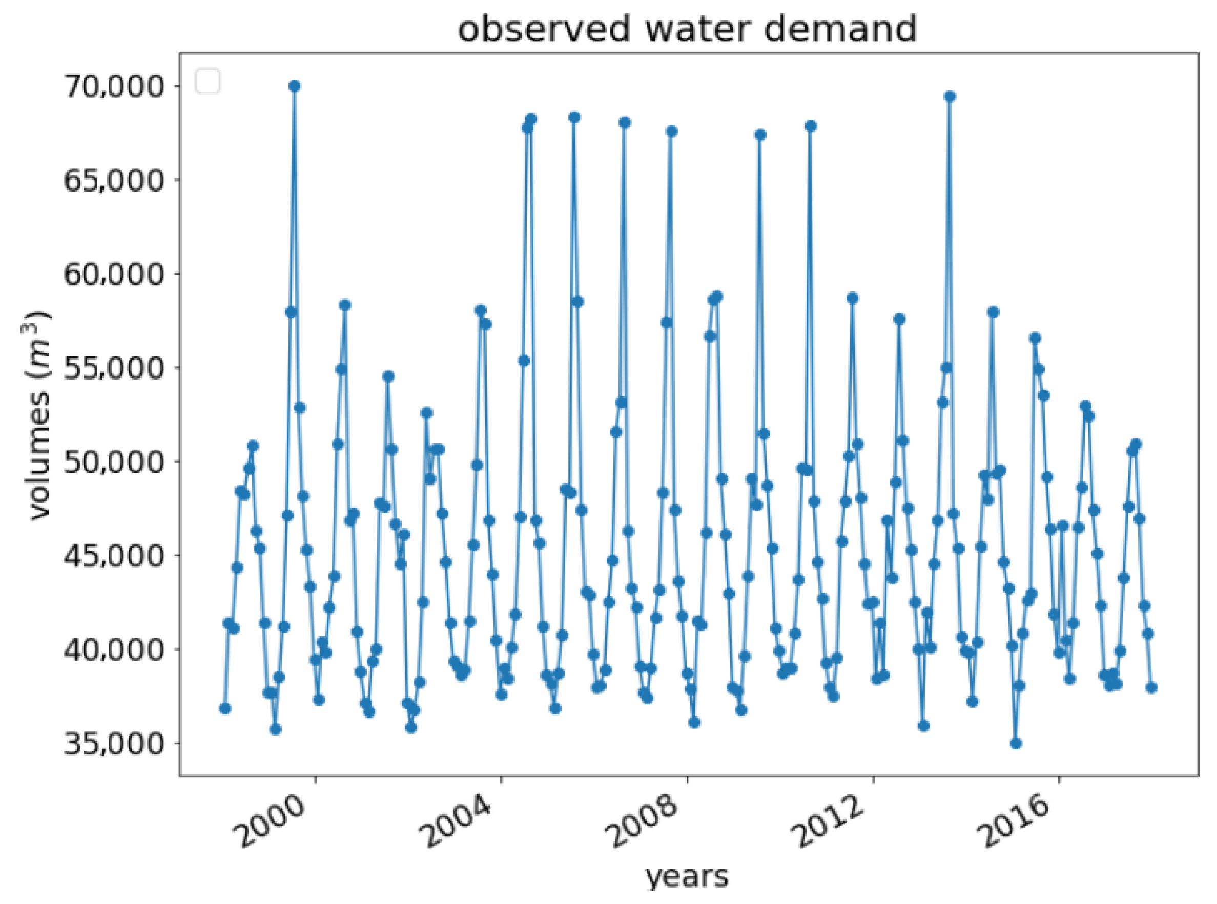
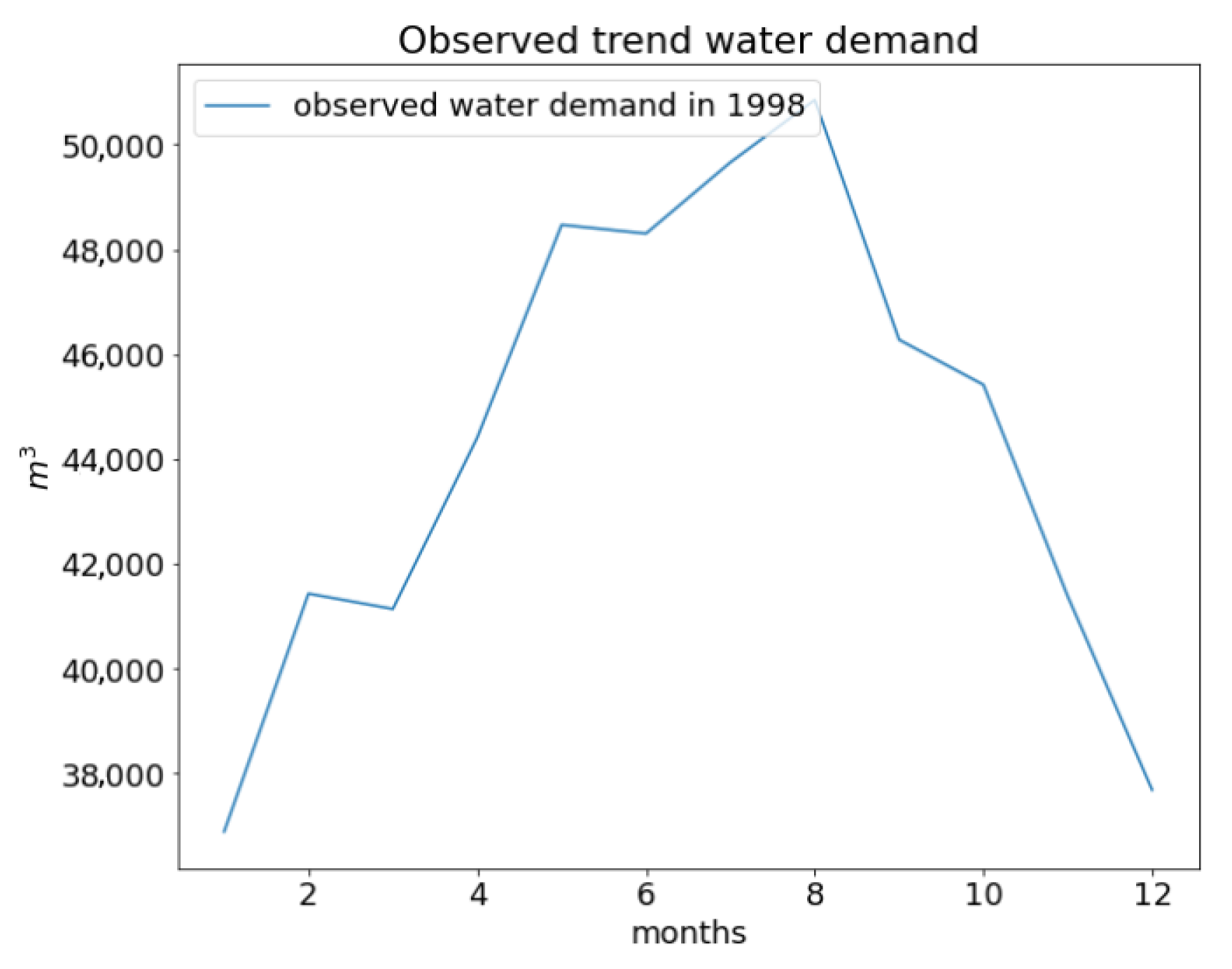
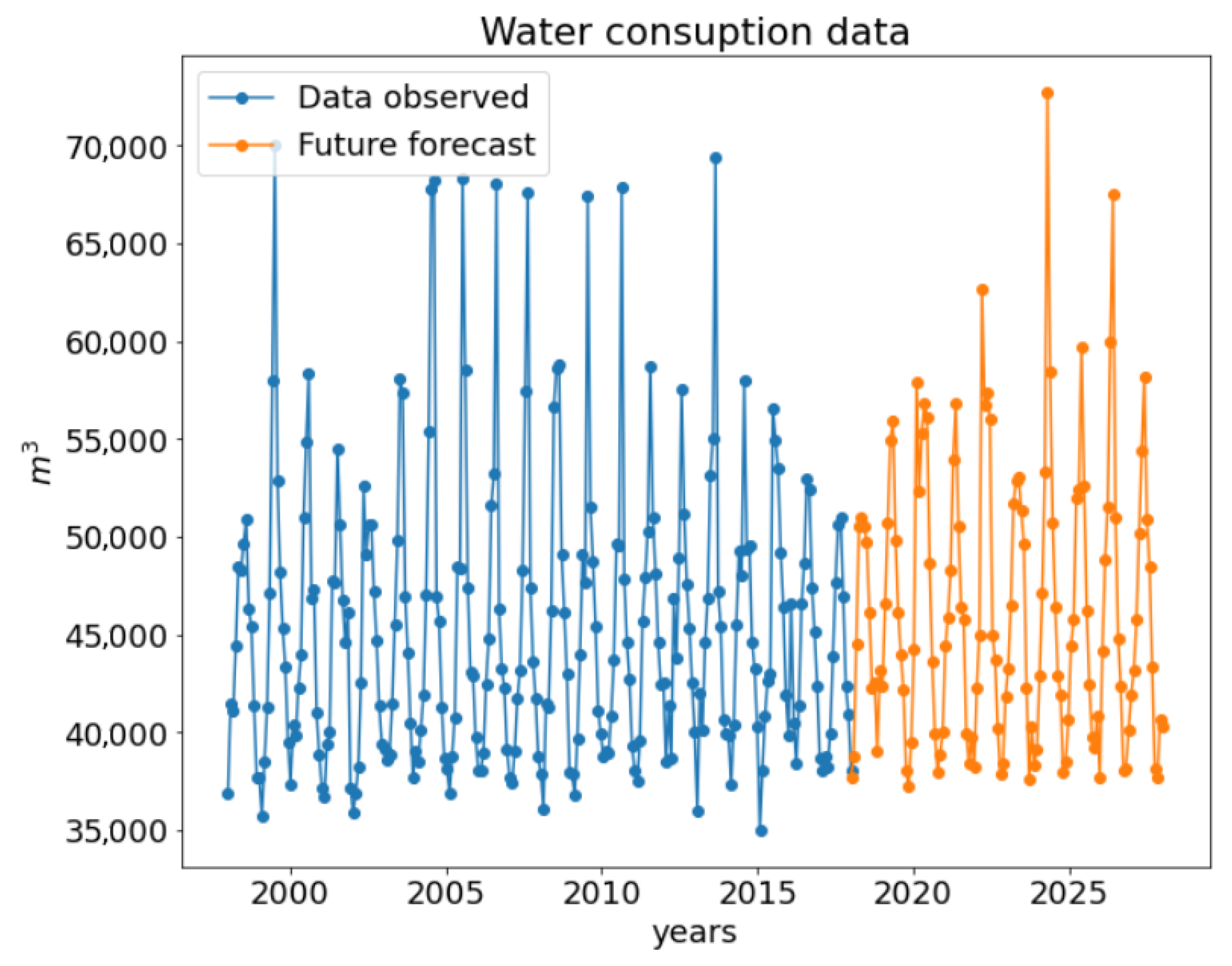
From 1998 to today, the consortium ACAVN [36], which manages the water supply to the town, surveyed the volumes entering the network, aiming at verifying the taxed volume. In the present study, these data are used for the calculation of the reservoir volume. Figure 3 shows the trend of the measured consumption [36].
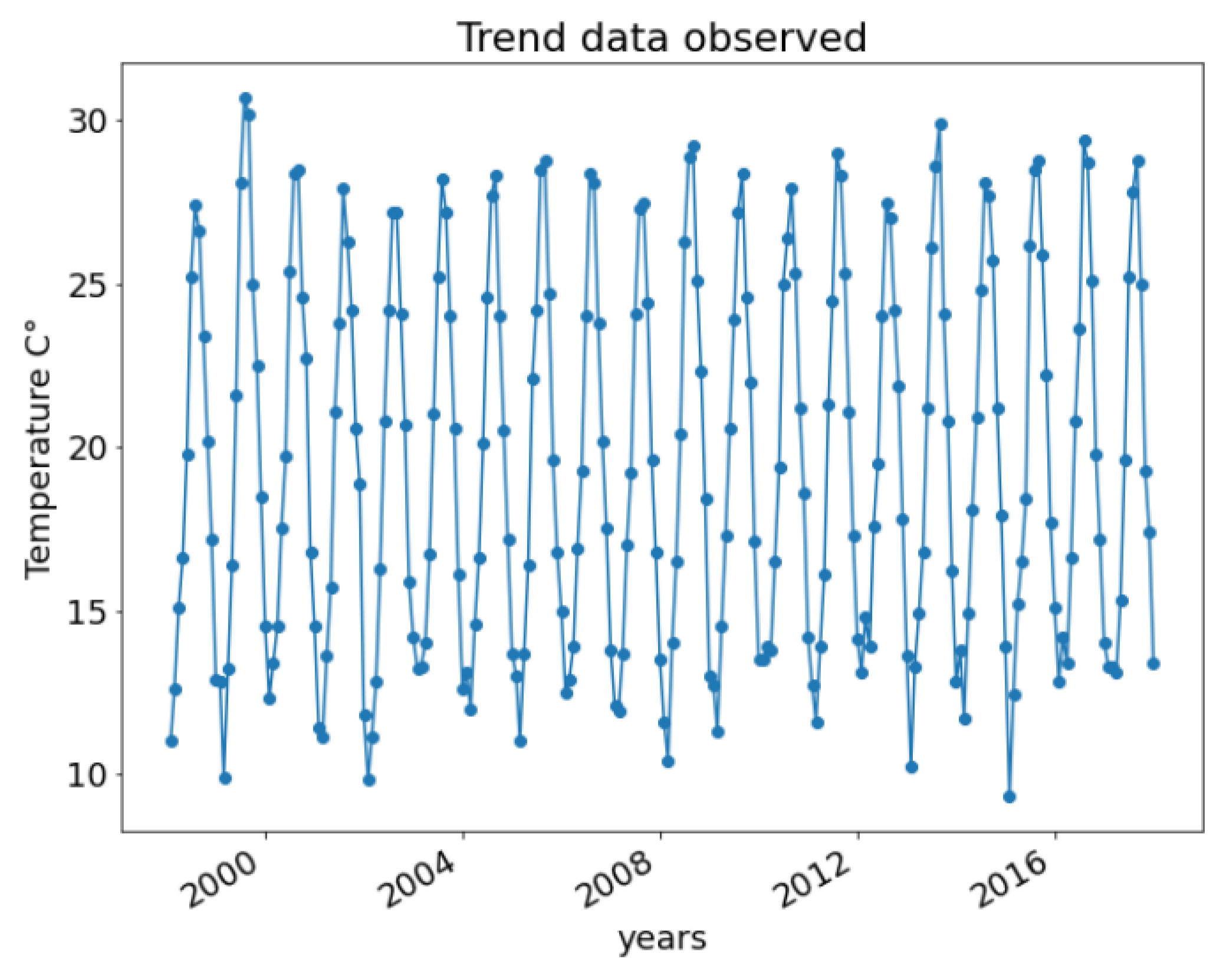
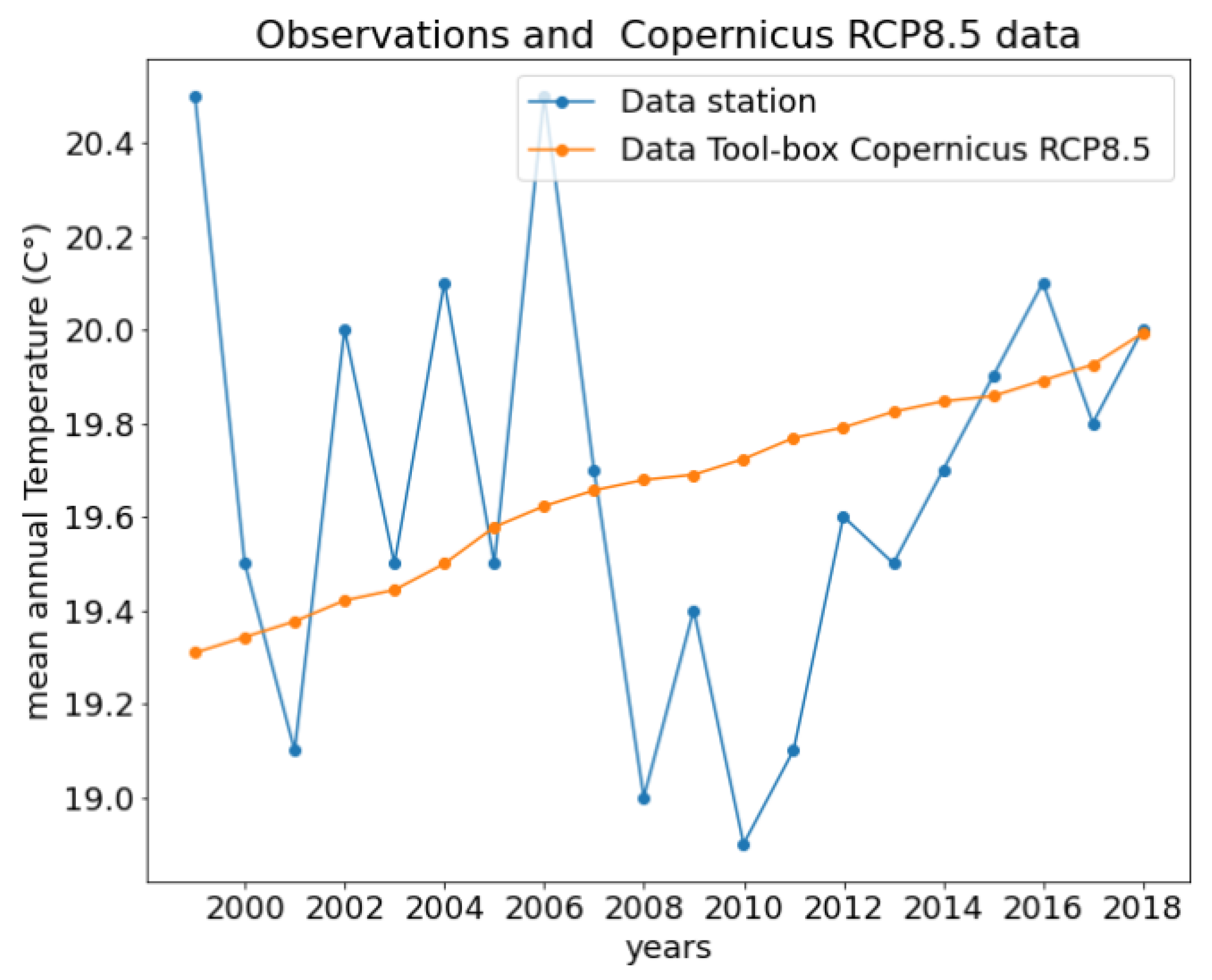
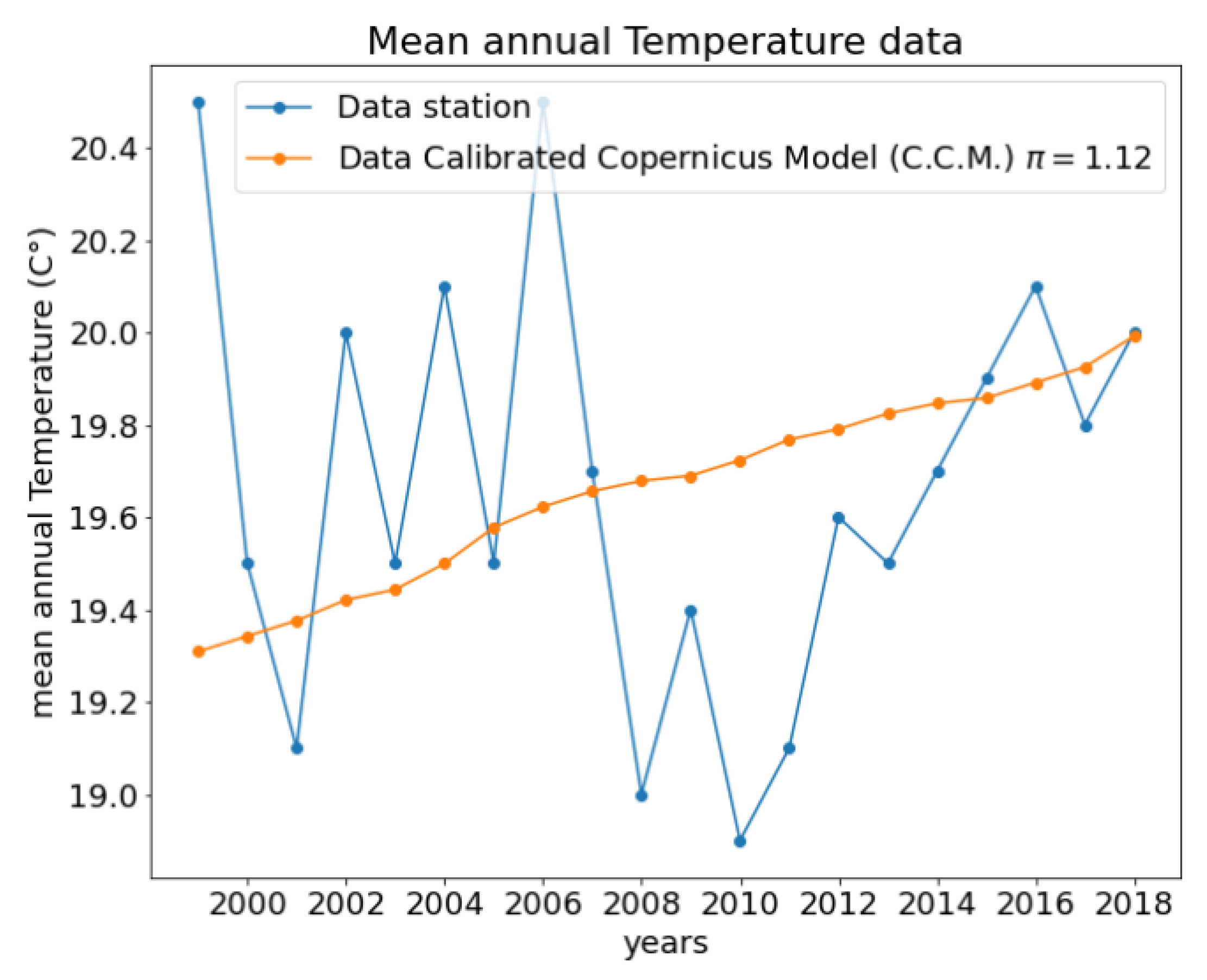
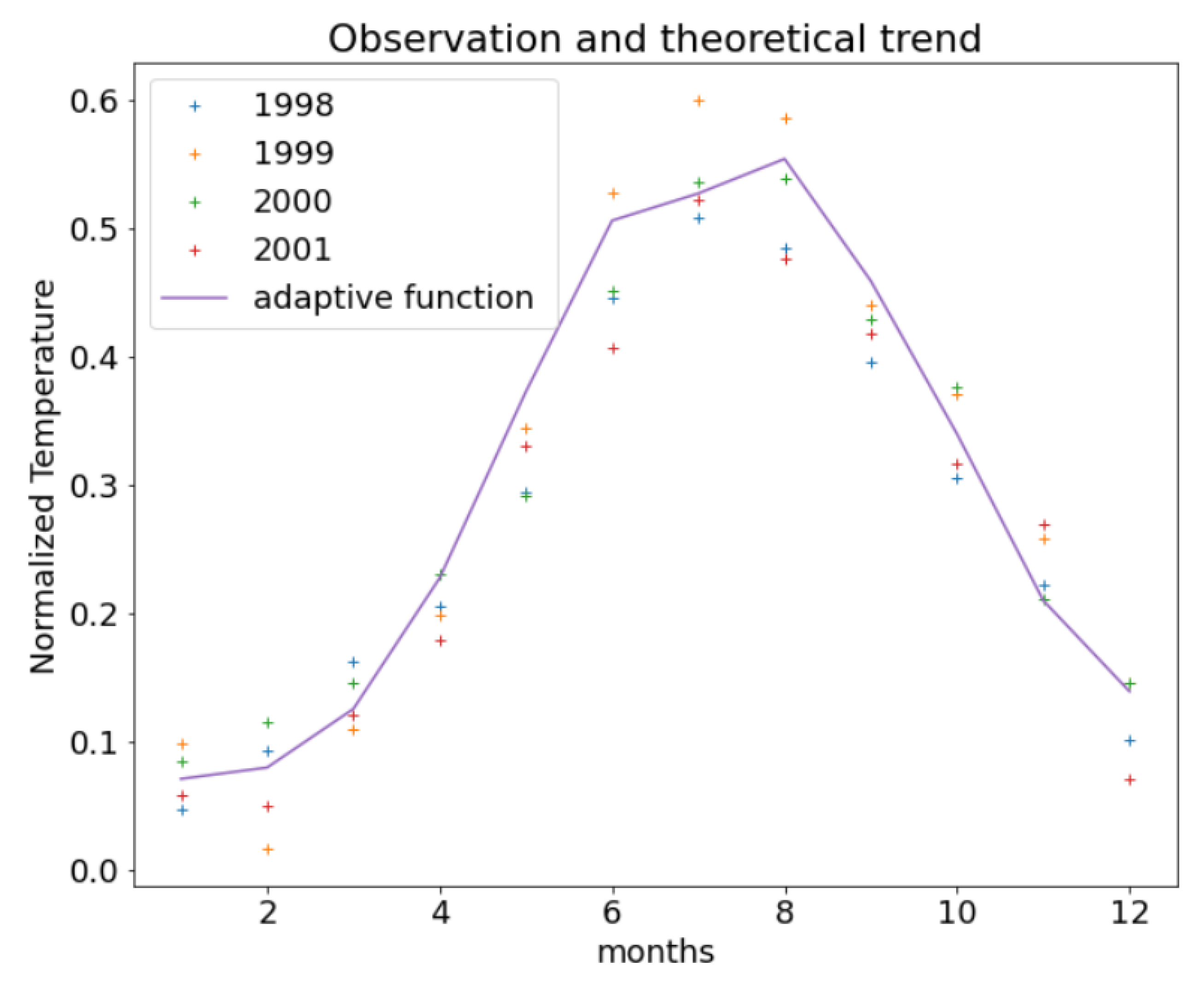
In addition, some environmental parameters, such as temperature data, number of users and number of rainy days per month were also considered, as these factors strongly influence the water demand. Temperature data, recorded by the weather station located in Messina (Geophysical Institute) were collected from [37], as they are the longest and most representative source for this site. Figure 4 shows the trend of the monthly temperatures of the last 20 years.
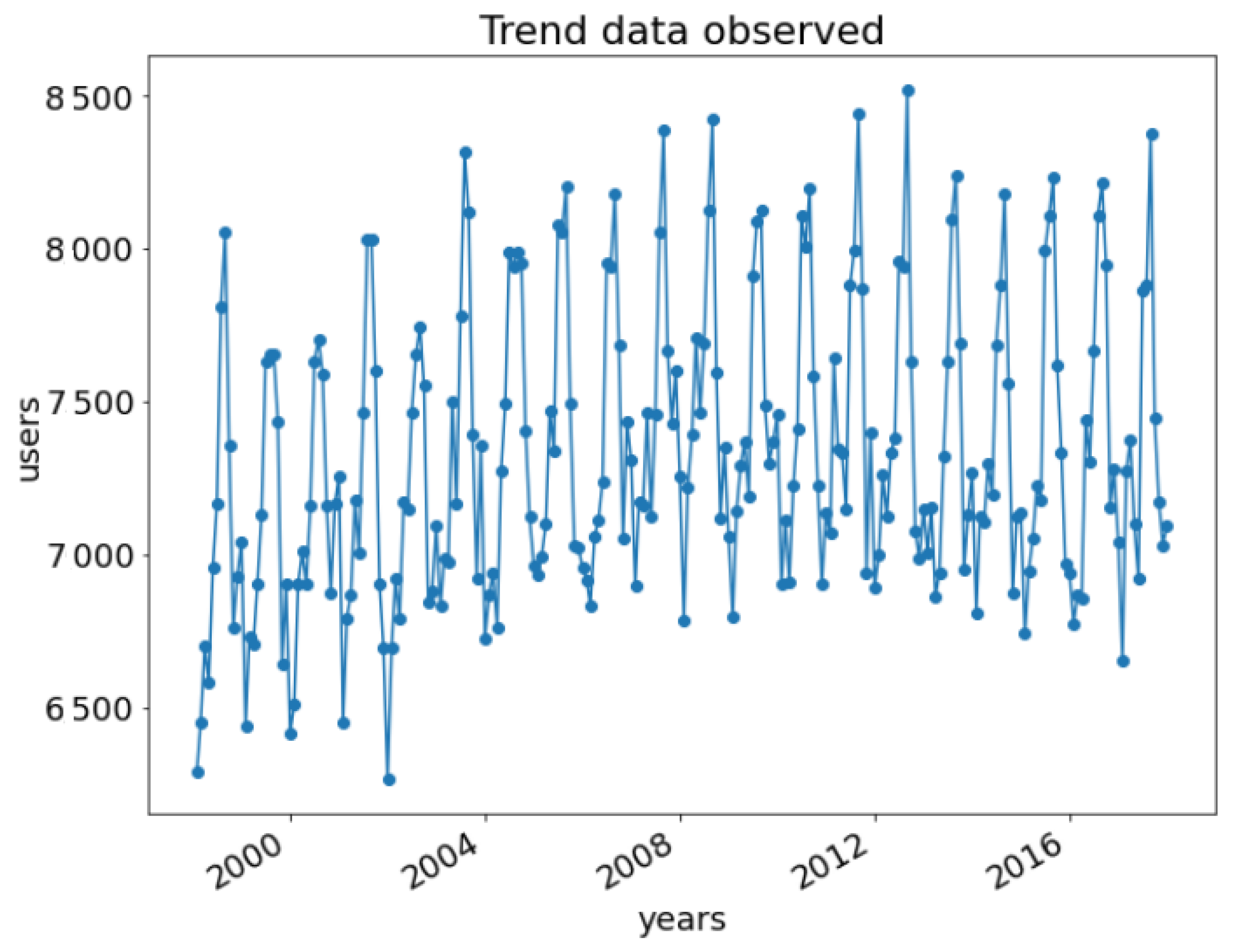
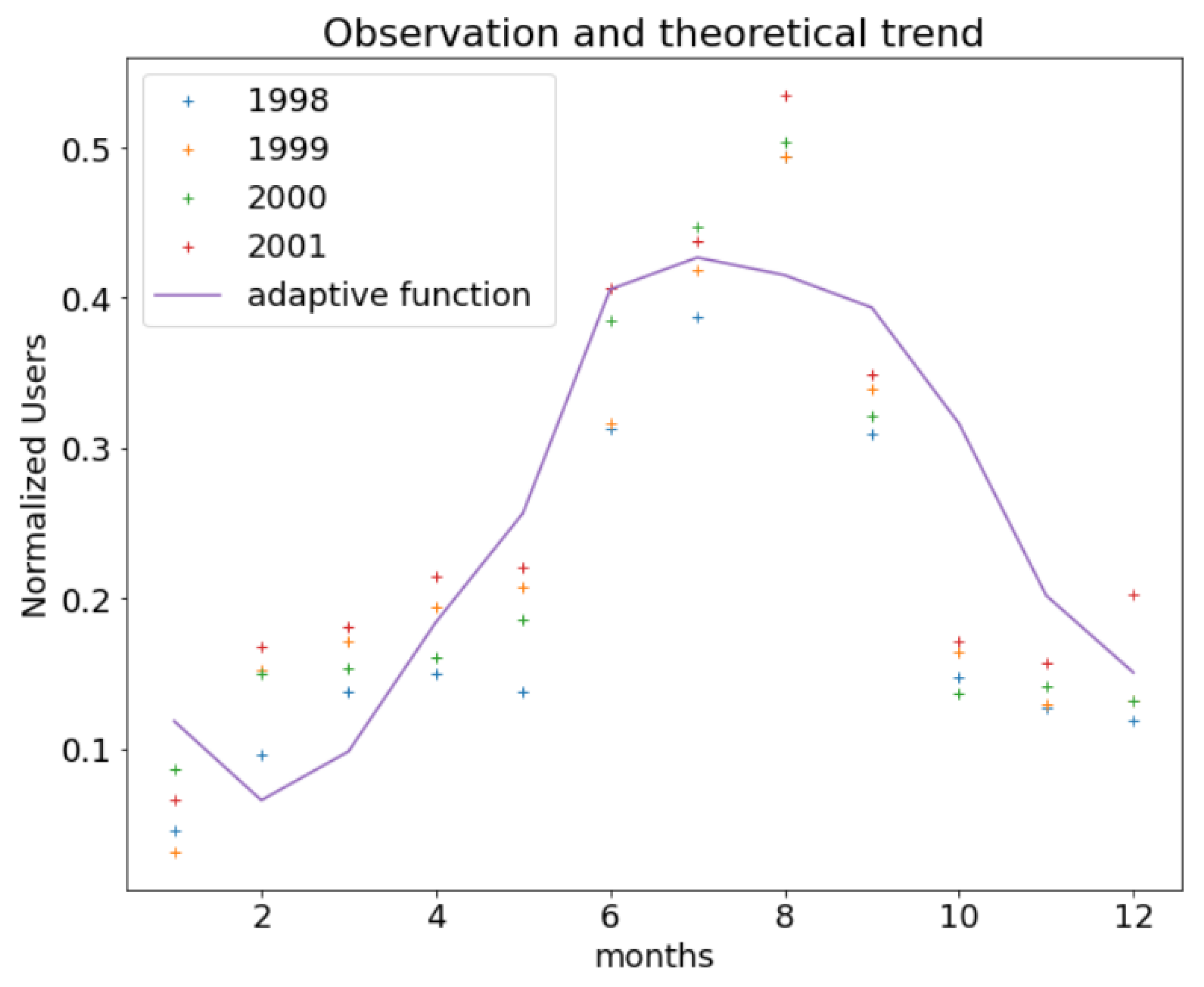
The population varies over time due to both weekly and monthly variability. Being a touristic area, the peak of the total users occurs during the month of August, while the opposite happens during the winter, leading to greater water demand in the summer. The data relating to users were obtained from the local registry office in combination with the data collected by Istat [38]. In particular, the number of total users was obtained as the sum of the resident population and the commuter or touristic population, which was obtained by an analysis conducted by the local city administration [39]. Figure 5 shows the trend of the total network users in the investigated period, where the number of commuters ranges between 1500 and 2000 persons.
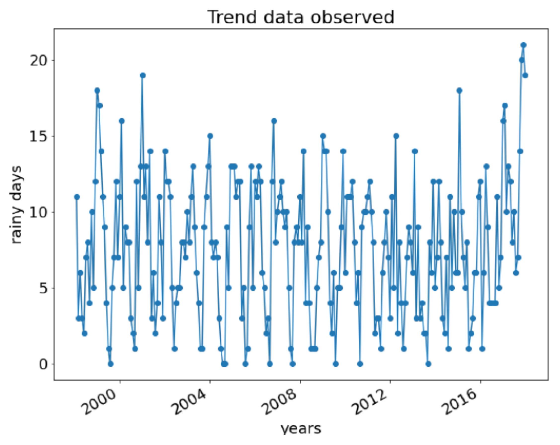
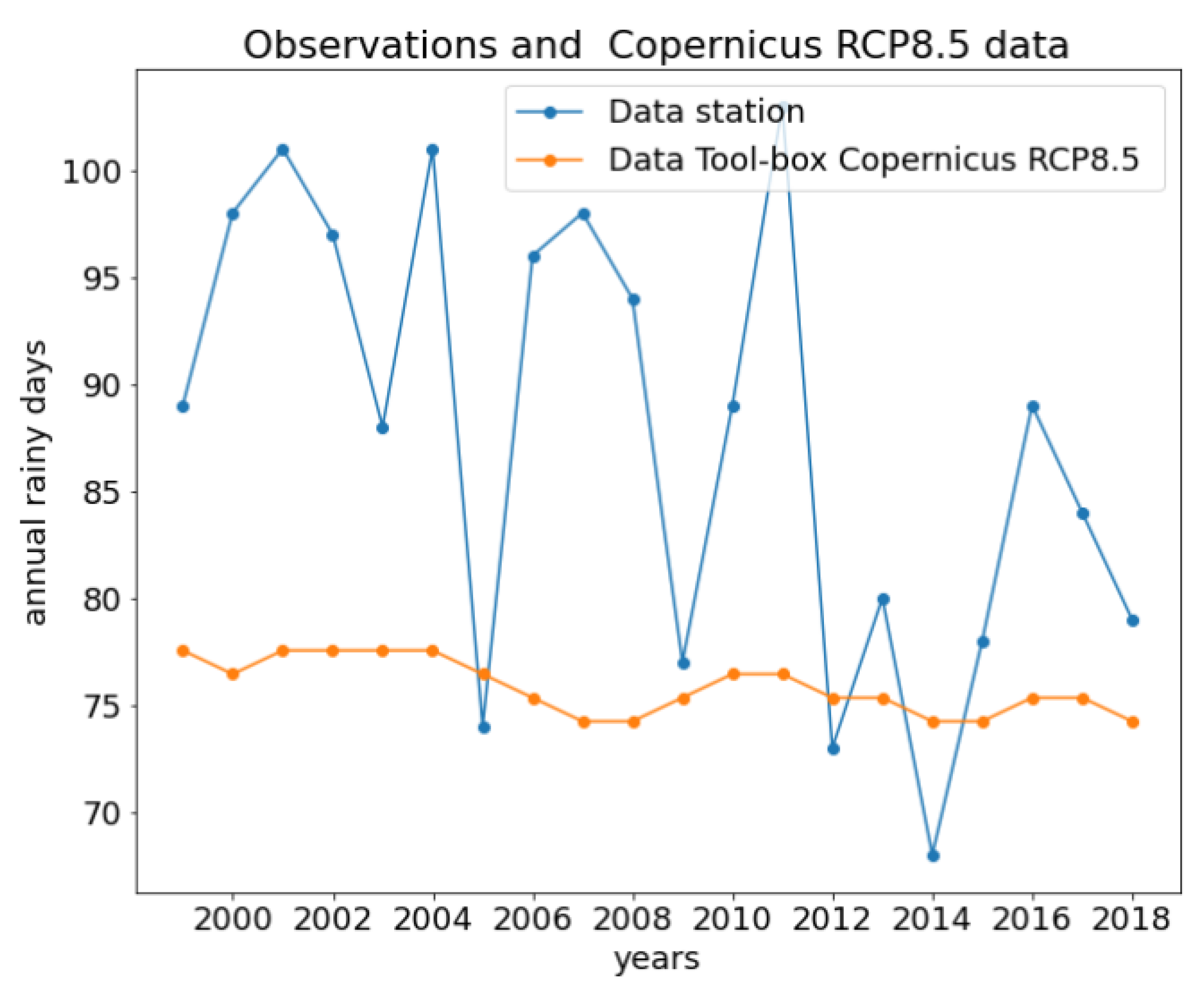
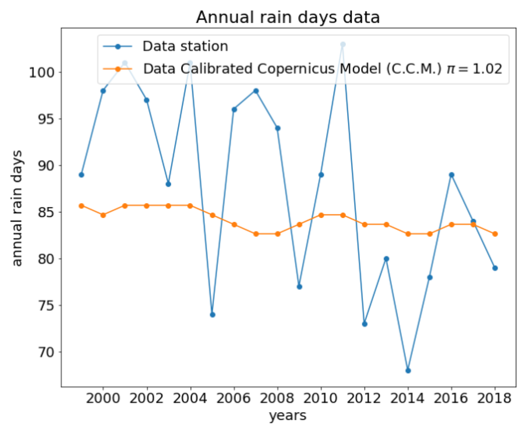
Finally, Figure 6 shows the number of rainy days per month in the investigated period. It is worth pointing out that, in the present study, a day is considered rainy when the cumulative precipitation reaches at least one millimeter during the 24 h. This choice is due according to the Copernicus service, which defines a “dry day” as a day when the threshold of one millimeter of cumulative precipitation is not exceeded in 24 h [40].
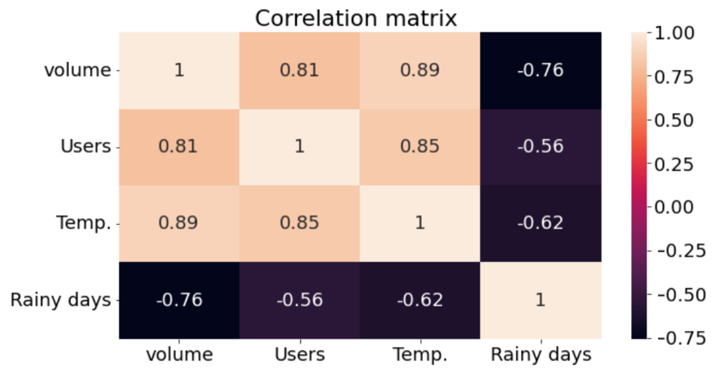
In order to verify the hypothesis of dependence between water consumption with the previously mentioned environmental parameters, the correlation matrix in Figure 7, reports the correlation factors between the water demand with the rainy days per month, the population and the temperature. It is possible to note that, though being correlated with water consumption, the previous environmental parameters cannot be expressed with an analytical function of the first variable.
This leads to considering the possibility to use a neural network approach in order to forecast the water supply as a function of all the parameters that can influence the water demand. In the following sections, the possibility to adopt an artificial neural network to define the water supply for the considered case study will be explored. Data coming from the trained ANN will serve as a benchmark to obtain the needed tank volume for satisfying the consumption.
3. Development of the ANN Model
3.1. Data Arrangement
The ANN model employed here is a multi-layer perception, i.e., a model comprising an input layer, hidden layers and an output layer [41]. The input layer allows the environmental parameters influencing the process to be considered. Domestic water usage over time is obtained as output. The hidden neurons are arranged into hidden layers, whose configuration depends on the problem to be faced and can be optimized as a function of the available dataset. In this specific case, the input layers are the three datasets of temperature, rainy days and population. First, the data were normalized according to the range between the minimum and maximum values:
where the and are, respectively, the maximum and minimum input values, while x is the generic input value. is the normalized value. Similarly, as far as the output is concerned:
where the and are, respectively, the maximum and minimum output values. The is the normalized value.
As mentioned before, in the present study, three input datasets were considered, specifically, the temperature, the monthly rainy days and the users served, while the total volume consumed over the month is the output.
3.2. Performance Evaluation
In order to develop the ANN Model, of the N data were used for training and for testing. Then, the root mean squared error , the Pearson correlation coefficient r and the determination coefficient were employed as performance indices of the models, which are shown and represented in the following.
where P and T are the predicted and target values, the bar indicates the average value, and S is the total number of training or testing samples. For building the neural network reported in this section, Tensorflow [42] and Keras [43] libraries were used.
3.3. ANN Efficiency
The efficiency of ANN models depends on the architecture of the neural network i.e., the number of hidden layers and the number of neurons. A single hidden layer architecture with a different number of neurons in the hidden layer was adopted for the ANN model as this structure generally leads to better results. It should be noted that, for a typical ANN algorithm, it is necessary to optimize the overall ANN structure before deciding the final number of hidden nodes.
Repeated training and testing should be performed with different ANN structures. On the one hand, if the number of hidden layers and/or hidden neurons is too high, there is a risk of over-fitting [44]; on the other hand, if their number is too low, this leads to under-fitting [45]. For the previous reasons, each model was run three times; then, the average values of , and r were determined for each ANN model. Table 1 shows the performance indices of the ANN models.
As can be seen in the table, selecting the number of 13 neurons can lead to better results by having the highest values of r and and the lowest value. Moreover, the network shows a good correlation between the training and testing data as reported in the following Table 2.
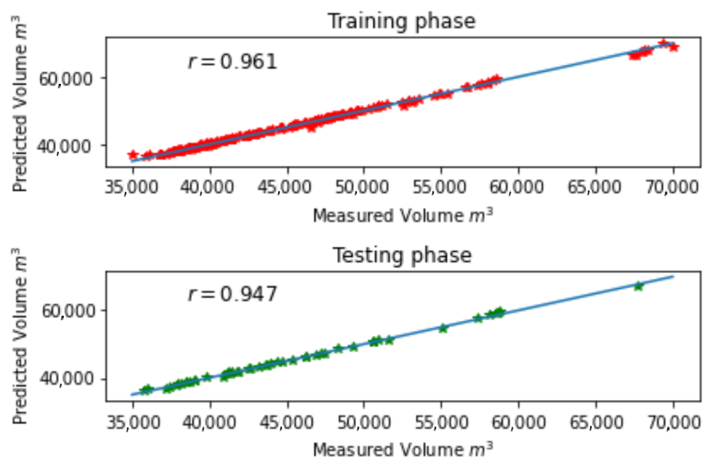
As shown in Figure 8, for the highest y values, the correlation becomes slightly worse, likely due to the difficulty in estimating the fluctuating population. From what is shown above, it is possible to confirm that the volumes of consumed water strongly depend on the temperature, on the days of rain and on the number of users served. This result was somewhat expected because there is a high percentage of users who live in houses with gardens or external spaces, as shown in Figure 9; hence, a large amount of water consumption is necessarily used to feed the green spaces in the hot and drought period. Furthermore, the habits of users are strongly influenced by temperatures. As shown in Figure 10, during the summer, a consumption peak is observed, which is due to the concurrent high number of users and hot temperatures.
Once the ANN is trained, it can be used in order to forecast forthcoming crisis events of the reservoirs. To this aim, it is particularly important to predict the environmental parameters accordingly. For population, a fitting interpolation starting from available data was used, while the other parameters were determined through the Copernicus platform as detailed in the next section.
4. Prediction of Environmental Variables
For the prediction of future data, a toolbox made available by the Copernicus platform was used [40]. In particular, the toolbox for biodiversity-climate-suitability was developed in 2022 with the aim of identifying multiple bio-climate indicators, among which, the temperature and drought days series are also considered [40]. Essentially, the latter quantities can also be determined for the past in order to be compared with the existing data.
Considering a RCP8.5 scenario [46], such an approach was applied to both rainy days and temperature for the period 1998–2018 to detect the trends as shown in Figure 11 and Figure 12, respectively. As well, the temperature and rainy days data are also superimposed on the same pictures. It is possible to notice from Figure 11 and Figure 12 that there are significant differences between the observed data and the trends proposed by the RCP8.5 model for the considered area.
In particular, it is possible to note a strong difference in temperatures, while a better agreement is shown on rainy days (Figure 12). Such discrepancies can be due to the fact that the scenario modeled by the Copernicus toolbox refers to a grid with a (1 × 1 km) resolution. It was, thus, necessary to calibrate the curves proposed by Copernicus with the data observed at the rainfall station.
In order to estimate each quantity, the coefficient , which minimizes the deviation between the observed data and the model data , was searched:
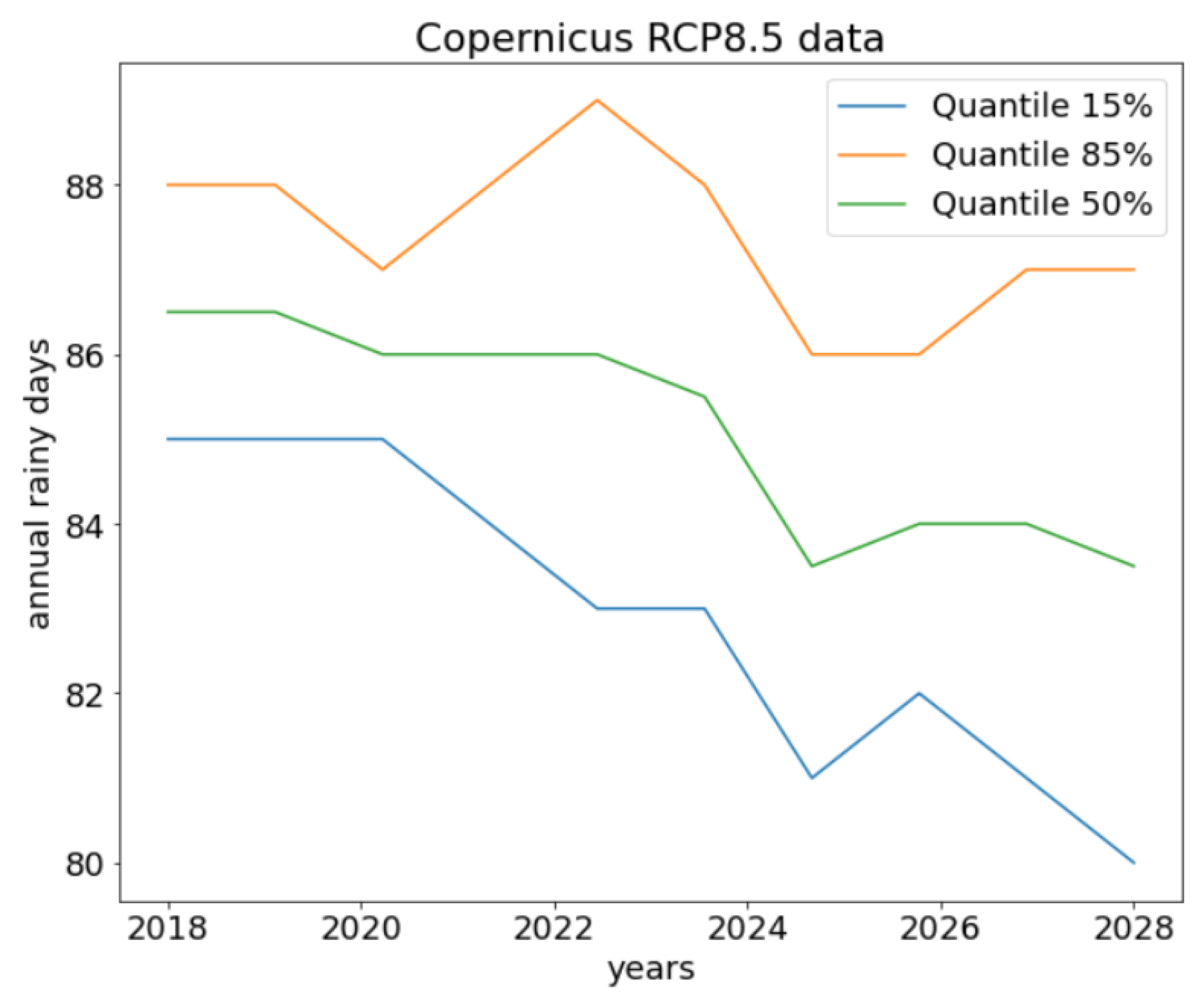
Figure 13 and Figure 14 show the comparisons between the observed data and the Copernicus estimate with the adoption of parameter . After the calibration, it is possible to note that the model well describes the observed data, at least in terms of the mean value. According to such an adaptation, Figure 15 and Figure 16 show the future trends of both rainy days and temperatures in terms of the median value predicted by the Copernicus-RCP8.5 model, together with the 15th and 85th quantiles.
4.1. From Yearly to Monthly Water Demand
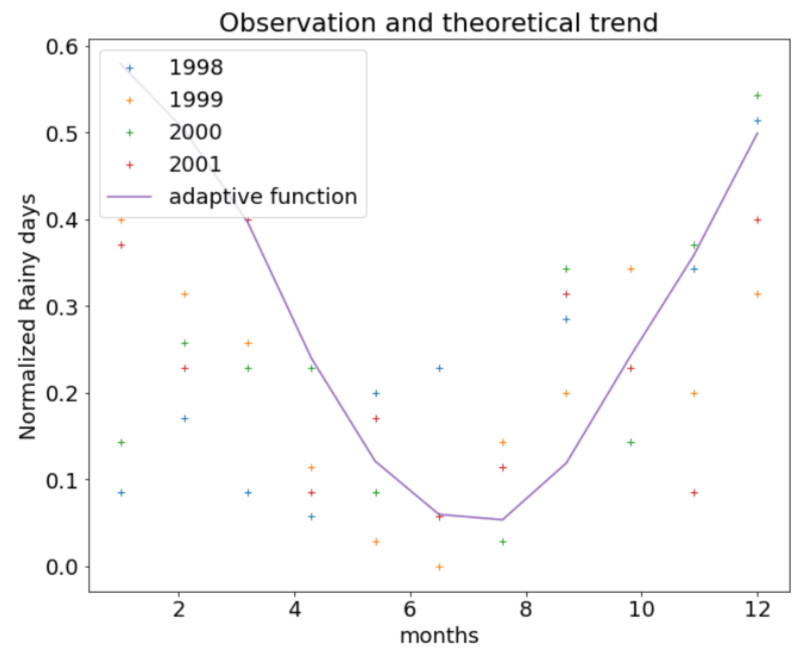
Once the average yearly trends were recovered, it was necessary to refer such values to a monthly scale through an adaptive function based on the observed quantities at the measuring station. The adaptive function was used for data on rainy days, temperatures and served users. This operation was performed through Equation (7), where indicates the monthly trend of both such quantities.
and are calibration coefficients to be obtained starting from the observed data, while and must respect the continuity of the annual data, i.e., the integral of the adaptive function must return a value congruent with the same prediction of the calibrated Copernicus model (C.C.M.). Moreover, is a random function that expresses the possible deviation from the average value . Finally, is a numerical interval, depending on the range of the 85th () and 15th () quantiles as predicted by the Copernicus- RCP8.5 scenario:
Figure 17, Figure 18 and Figure 19 show the comparisons between the function reported in Equation (7) and the data observed at the reference station. The Equation (7) model is well suited for data relating to temperature, while it shows some scatter for data on population and rainy days, due to the fact that the latter two assume a less regular monthly trend in the observations.
Regarding the population, we assumed that it will undergo a decrease of in the next 10 years as stated by the global analysis conducted by Istat [47]. In addition, the suggested trend on DEMO-Istat [38] on the studied location confirms this tendency. In particular, for the town of Torregrotta, the decrease began in 2014.
All the previously obtained data for the next 10 years were considered as the input data of the trained network. The results are shown in Figure 20, where the future prediction of consumption on a 10-year time scale is reported along with the observed data.
4.2. From Monthly to Hourly Water Demand
Once the monthly consumption was obtained, it is convenient to switch to hourly consumption. This procedure is entirely theoretical; therefore, it requires, as inputs, the existing observations and literature data [48]. Specifically, the first step is to obtain the daily consumption in 24 h, through a peak shape function that identifies different peak consumption within a month:
where the t is expressed in days, the index i sums over 4, i.e., the number of weeks as well as the peaks per month. The maximum of is reached on Saturday, when the urban district welcomes worker users coming from the neighboring towns. indicates the peak position, represents the extremities at each side of the peak, and is a term introduced for sake of continuity.
Essentially, the sum of the monthly consumption must satisfy the prediction of C.C.M. according to Equation (10):
Based on Equation (10), it is possible to define the previously introduced coefficients by means of the following system of Equation (11):
The results of the mentioned approach are synthesized in Figure 21, where the non-dimensional daily volume, made non-dimensional by means of the Saturday peak volume, is plotted.
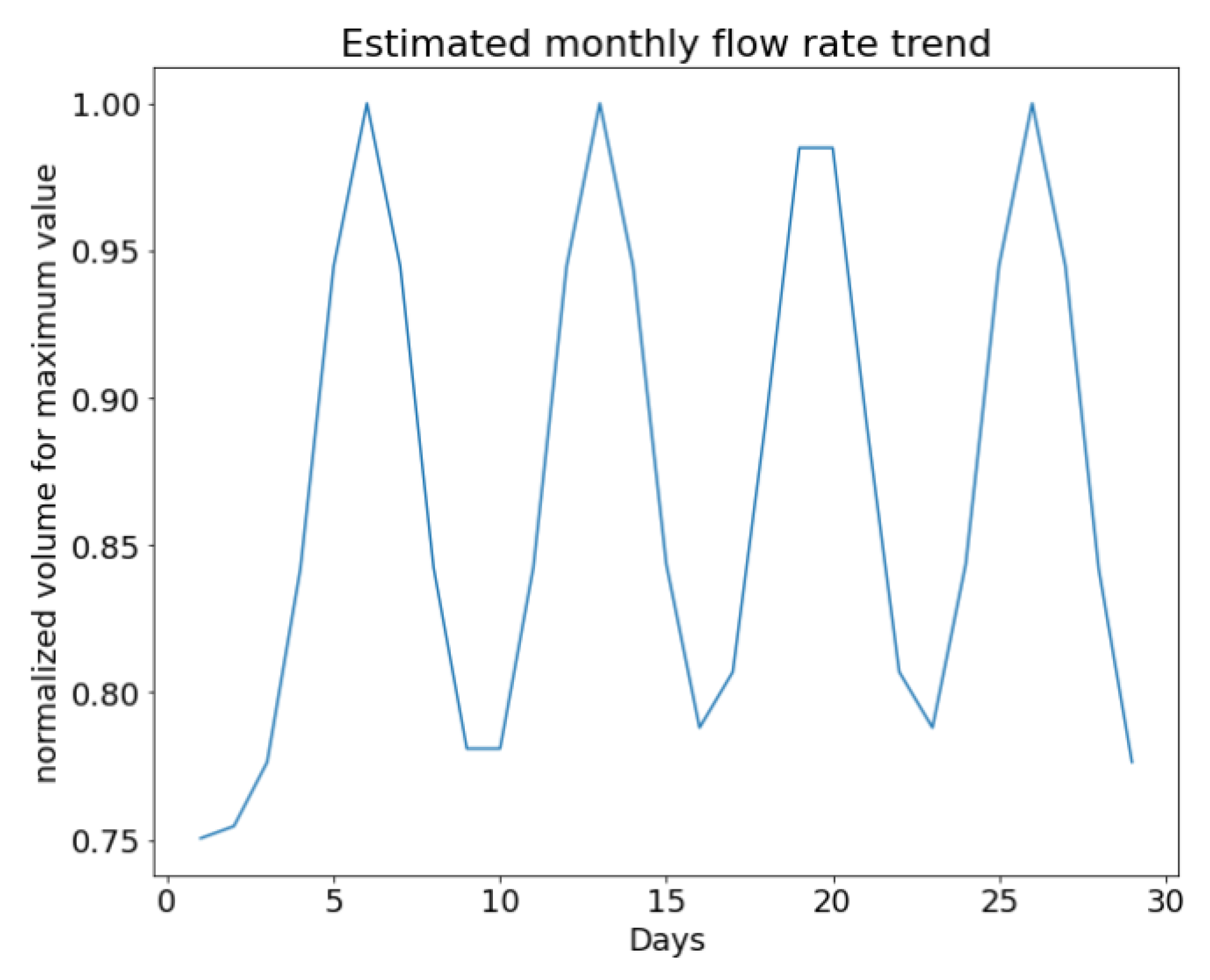
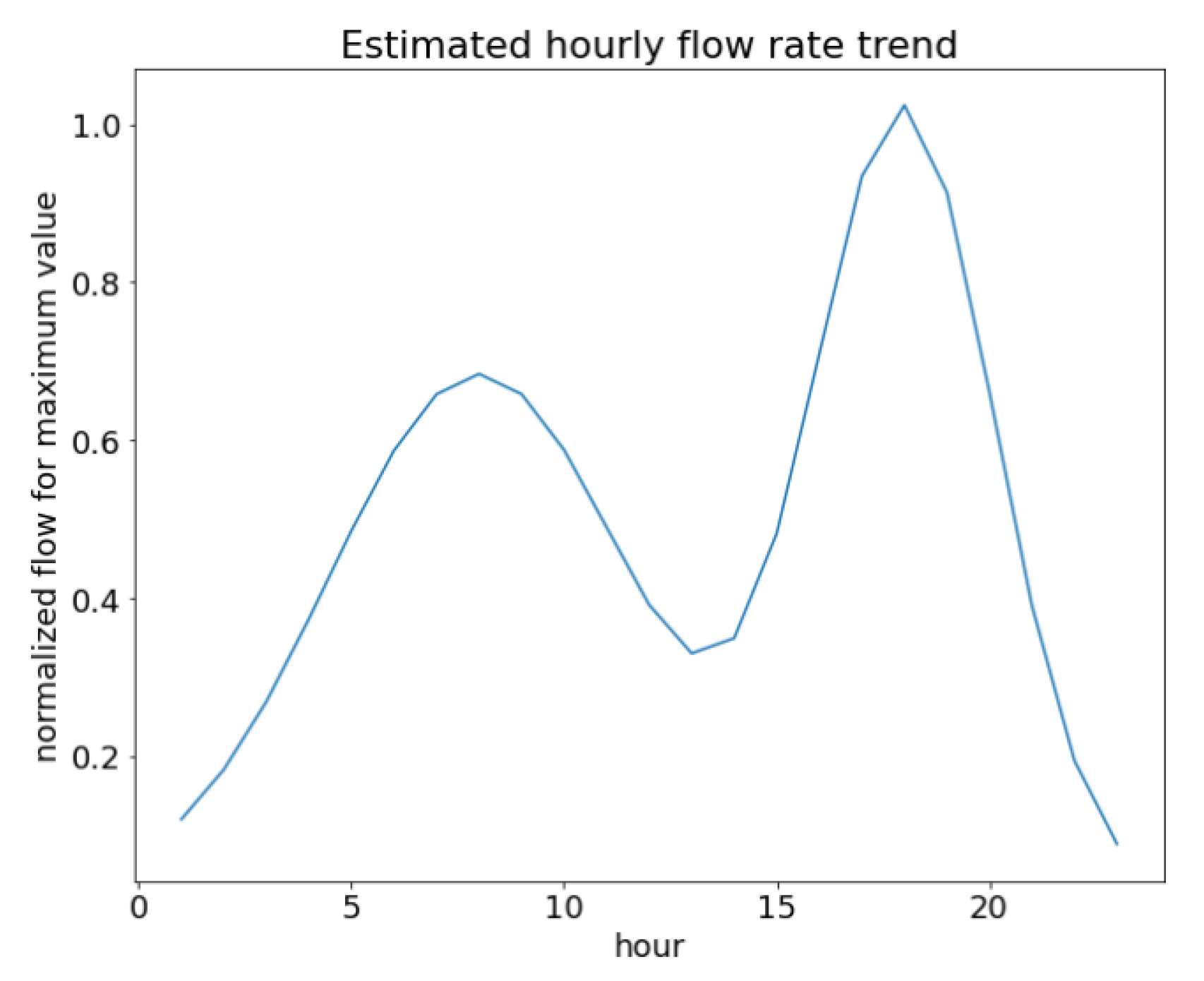
In the same way, the equation of the hourly consumption trend was obtained, considering that the peaks occur at 18:00 and at 8:00 [3]. Furthermore, as the inhabitants of the district total about 7000, the hourly peak coefficient was assumed equal to 3 [3]. The adopted relation is reported below:
where the t is expressed in hours, and k is the number of peaks per day, equal to 2.
Similarly to Equation (9), Equation (12) must also satisfy compatibility on a daily scale with volumes. Therefore, an integral is imposed that is equal to the total daily volume (Equation (13)).
The resolution of the previous problem leads to the following solution:
The results of the mentioned approach are synthesized in Figure 22, where the hourly volume, normalized by means of its maximum value, is plotted showing the two peaks as indicated before.
Regarding the water flowing into the reservoir to be sized, it was necessary to assume that the input volume varied randomly around its average value [49]. To this aim, it is possible to assume that -1 and -2, being connected in a series, can be represented as a unique tank with an equivalent volume, equal to the sum of the two. In this way, can be referred to as the equivalent volume. Equation (14) was, thus, applied to the entire simulated period, while Figure 23 plots the results for a one-month period.
5. Sizing of the Reservoir Volume
The variability of the volumes stored in the equivalent tank was calculated through the numerical integration of Equation (15):
where is the hourly flow determined through Equation (12), is the hourly inlet flow Equation (14), and is the time-series length. The physical limit conditions impose a minimum value of 0 and a maximum equal to the total volume of the equivalent tank as reported below.
Equation (15) can, thus, be solved through numerical integration at finite differences, i.e.,
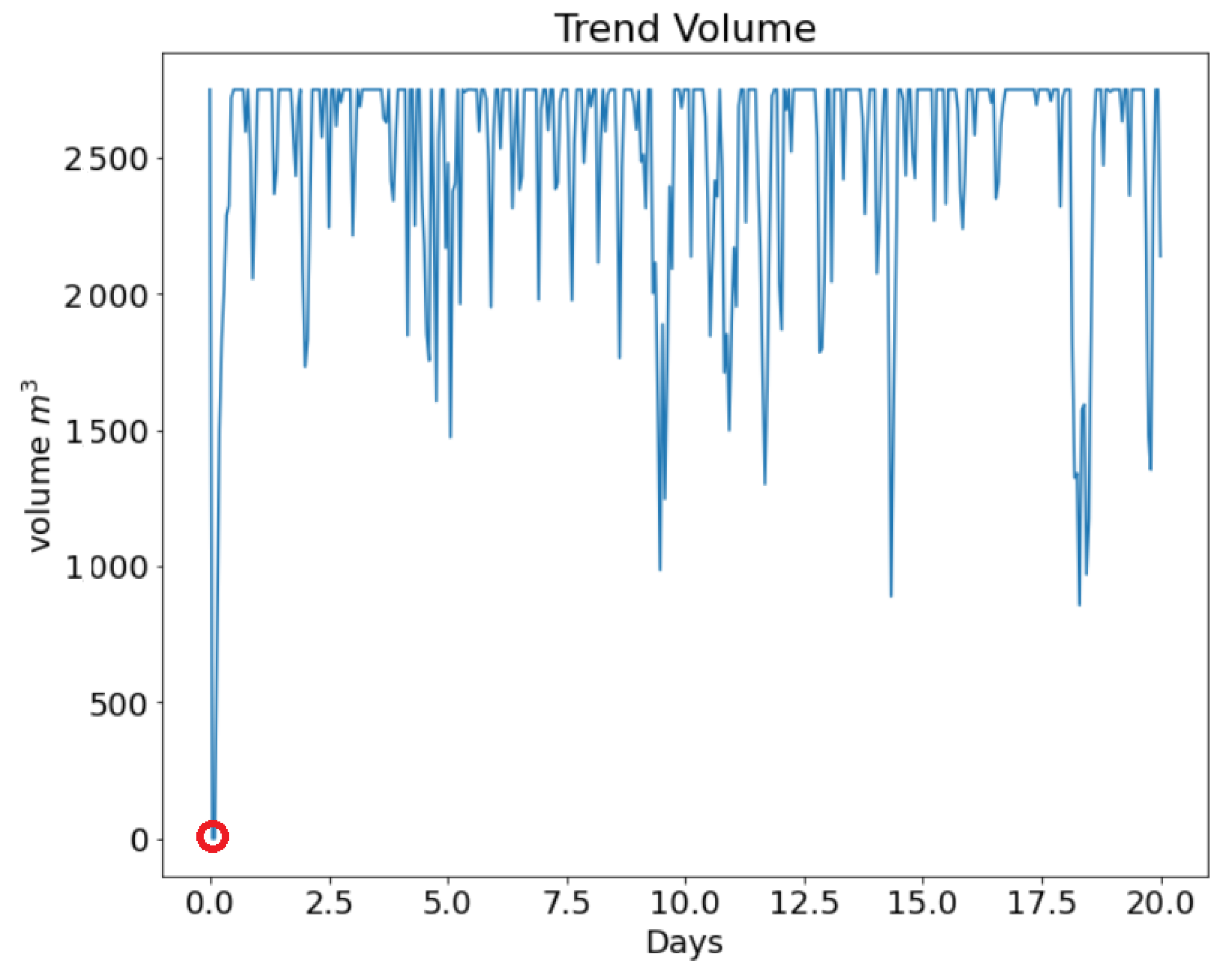
The series begins when the tank is full, i.e., ; therefore, it is possible to impose as the initial condition and to evaluate the total crisis hours in the time series corresponding to the simulated 10 years. The tank crisis hours will be the instants in which the tank volume equals 0. The results are plotted in Figure 24. Here, the time series of the volume is shown for a period of 20 days, and the red circle denotes the crisis event occurring during the selected period.
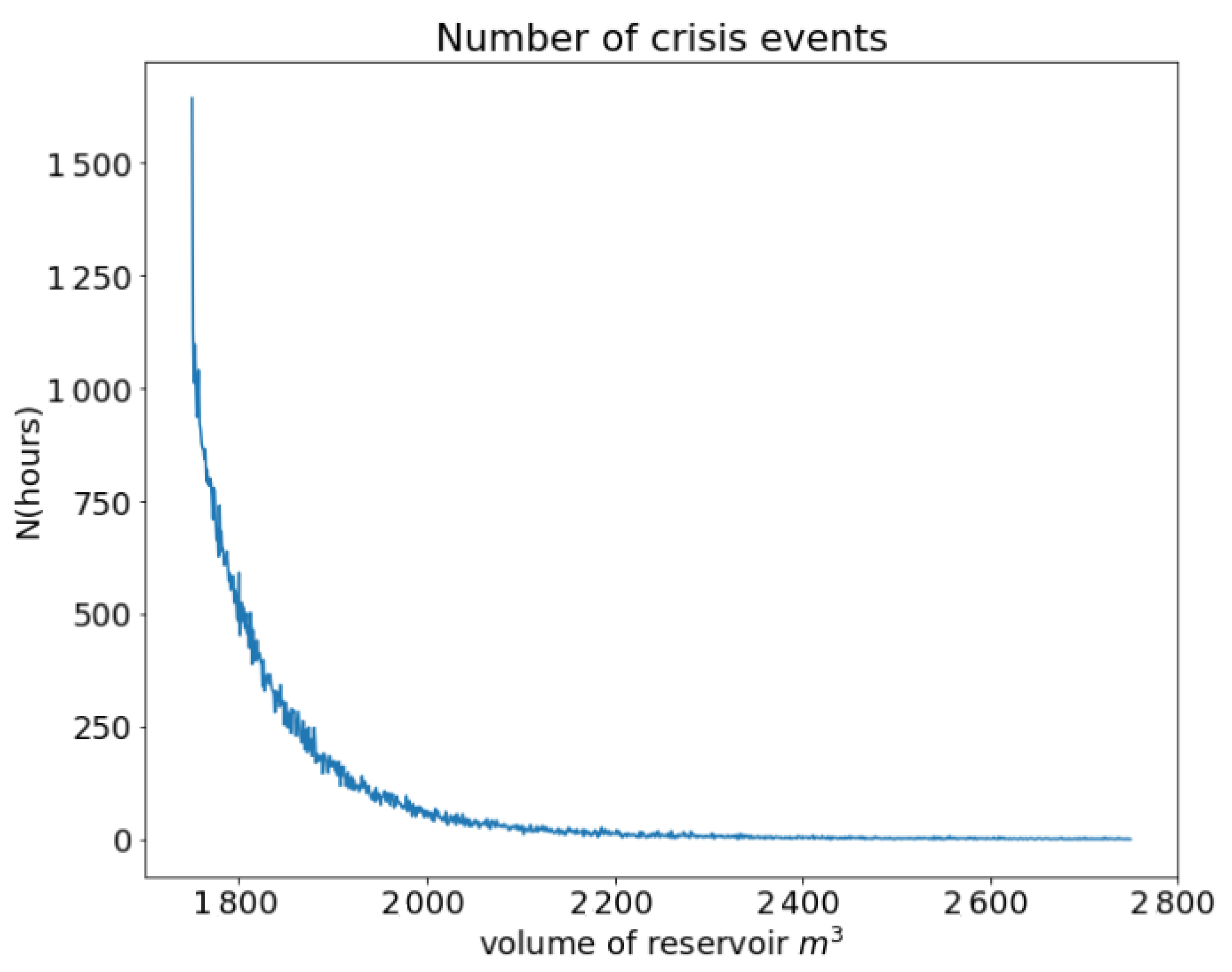
The same operation was repeated as changed in order to check the number N of crisis events during the simulated period. As is possible to observe in Figure 25, N decreases with an exponential law with the increasing of the tank volume. Hence, it is possible to identify an optimal tank volume once an acceptable number of crisis events is fixed. In particular, in the present case study, it can be observed that the number of crisis events tends to remain approximately constant for volumes higher than 2200 m. This fact leads us to conclude that the choice of reservoirs larger than this, while also being uneconomical, does not result in a further reduction of critical episodes.
6. Conclusions
This paper proposed a new theoretical methodology to calculate the volume of an urban reservoir serving a civil network. First, data on the consumption, temperature, rainy days and number of served users were acquired. The future forecast of such environmental parameters was determined on the basis of the Copernicus service over the next 10 years. The resulting trends were applied for training an ANN with the aim of recovering the water consumption as output. Furthermore, through theoretical equations, the monthly flow rate was transformed into an hourly flow.
Numerical integration of continuity equations applied to reservoirs was then conducted to define the inlet flow. From the obtained results, it can be inferred that the number of crisis events, identified as the time steps in which the volume of the tank reaches zero, decreased exponentially toward zero as the reservoir volume increased. However, over a certain reservoir size, it became ineffective to further increase the volume to reduce the number of critical episodes. Hence, considering different total volume scenarios, this approach led to an optimization procedure that allowed the total volume of the reservoir to be determined once the number of crisis events was fixed.
Compared to other methods already used in the literature, the present approach does not explicitly consider the volumes required for different needs, such as fire protection, reserve or compensation; thus, it is suitable in applications involving small urban reservoirs.
Author Contributions
Conceptualization, B.S. and C.F.; methodology, B.S.; software, B.S.; validation, C.F.; investigation, B.S.; resources, C.F.; writing—original draft preparation, B.S.; writing—review and editing, C.F.; supervision, C.F. All authors have read and agreed to the published version of the manuscript.
Funding
This research received no external funding.
Data Availability Statement
All the data used for the present research can be found at the referenced links.
Conflicts of Interest
The authors declare no conflict of interest.
References
- UNESCO. The United Nations World Water Development Report 2015: Water for a Sustainable World; Technical Report Water and Climate Change; UNESCO: Paris, France, 2015. [Google Scholar]
- Ehsani, N.; Vörösmarty, C.J.; Fekete, B.M.; Stakhiv, E.Z. Reservoir operations under climate change: Storage capacity options to mitigate risk. J. Hydrol. 2017, 555, 435–446. [Google Scholar] [CrossRef]
- Milano, V. Acquedotti; Hoepli Editore: Milano, Italy, 1996. [Google Scholar]
- van Zyl, J.E.; Piller, O.; Le Gat, Y. Sizing municipal storage tanks based on reliability criteria. J. Water Resour. Plan. Manag. 2008, 134, 548–555. [Google Scholar] [CrossRef]
- Assessorato Regione Sicilia. Piano di Tutela delle Acque, Sicilia; Assessorato Regione Sicilia: Sicily, Italy, 1999. [Google Scholar]
- Margaritora, G.; Moriconi, P. Consumi idropotabili del comune di Roma. In Proceedings of the La Conoscenza Dei Consumi Per Una Migliore Gestione Delle Infrastrutture Acquedottistiche, Sorrento, Italy, 9–10 September 1990; pp. 9–11. [Google Scholar]
- Stańczyk, J.; Kajewska-Szkudlarek, J.; Lipiński, P.; Rychlikowski, P. Improving short-term water demand forecasting using evolutionary algorithms. Sci. Rep. 2022, 12, 13522. [Google Scholar] [CrossRef]
- Chen, J.; Boccelli, D. Demand Forecasting for Water Distribution Systems. Procedia Eng. 2014, 70, 339–342. [Google Scholar] [CrossRef]
- Hemati, A.; Rippy, M.A.; Grant, S.B.; Davis, K.; Feldman, D. Deconstructing Demand: The Anthropogenic and Climatic Drivers of Urban Water Consumption. Environ. Sci. Technol. 2016, 50, 12557–12566. [Google Scholar] [CrossRef] [PubMed]
- Ghisi, E. Parameters influencing the sizing of rainwater tanks for use in houses. Water Resour. Manag. 2010, 24, 2381–2403. [Google Scholar] [CrossRef]
- Okeola, O.; Balogun, S. Estimating a municipal water supply reliability. Cogent Eng. 2015, 2, 1012988. [Google Scholar] [CrossRef]
- Georgakakos, A.P.; Marks, D.H. A new method for the real-time operation of reservoir systems. Water Resour. Res. 1987, 23, 1376–1390. [Google Scholar] [CrossRef]
- Koutsoyiannis, D. A Monte Carlo approach to water management. In Proceedings of the Geophysical Research Abstracts, European Geosciences Union General Assembly, Vienna, Austria, 22–27 April 2012; Volume 14. [Google Scholar]
- Marton, D.; Stary, M.; Menšik, P. The influence of uncertainties in the calculation of mean monthly discharges on reservoir storage. J. Hydrol. Hydromech. 2011, 59, 228–237. [Google Scholar] [CrossRef]
- Psarrou, E.; Tsoukalas, I.; Makropoulos, C. A Monte-Carlo-Based Method for the Optimal Placement and Operation Scheduling of Sewer Mining Units in Urban Wastewater Networks. Water 2018, 10, 200. [Google Scholar] [CrossRef]
- Sieber, J.; Yates, D.; Huber Lee, A.; Purkey, D. WEAP: A demand priority and preference driven water planning model: Part 1, model characteristics. Water Int. 2005, 30, 487–500. [Google Scholar]
- Sigvaldson, O.T. A simulation model for operating a multipurpose multireservoir system. Water Resour. Res. 1976, 12, 263–278. [Google Scholar] [CrossRef]
- Klipsch, J.D.; Evans, T.A. Reservoir operations modeling with HEC-ResSim. In Proceedings of the Third Federal Interagency Hydrologic Modeling Conference, Reno, NV, USA, 2–5 April 2006; Volume 3. [Google Scholar]
- Kim, J.; Read, L.; Johnson, L.E.; Gochis, D.; Cifelli, R.; Han, H. An experiment on reservoir representation schemes to improve hydrologic prediction: Coupling the national water model with the HEC-ResSim. Hydrol. Sci. J. 2020, 65, 1652–1666. [Google Scholar] [CrossRef]
- Lévite, H.; Sally, H.; Cour, J. Testing water demand management scenarios in a water-stressed basin in South Africa: Application of the WEAP model. Phys. Chem. Earth Parts A/B/C 2003, 28, 779–786. [Google Scholar] [CrossRef]
- Yates, D.; Sieber, J.; Purkey, D.; Huber-Lee, A. WEAP21—A Demand-, Priority-, and Preference-Driven Water Planning Model. Water Int. 2009, 30, 487–500. [Google Scholar] [CrossRef]
- Draper, A.J.; Munévar, A.; Arora, S.K.; Reyes, E.; Parker, N.L.; Chung, F.I.; Peterson, L.E. CalSim: Generalized model for reservoir system analysis. J. Water Resour. Plan. Manag. 2004, 130, 480–489. [Google Scholar] [CrossRef]
- Draper, A.J.; Lund, J.R. Optimal hedging and carryover storage value. J. Water Resour. Plan. Manag. 2004, 130, 83–87. [Google Scholar] [CrossRef]
- Zhang, D.; Lin, J.; Peng, Q.; Wang, D.; Yang, T.; Sorooshian, S.; Liu, X.; Zhuang, J. Modeling and simulating of reservoir operation using the artificial neural network, support vector regression, deep learning algorithm. J. Hydrol. 2018, 565, 720–736. [Google Scholar] [CrossRef]
- Hejazi, M.I.; Cai, X. Input variable selection for water resources systems using a modified minimum redundancy maximum relevance (mMRMR) algorithm. Adv. Water Resour. 2009, 32, 582–593. [Google Scholar] [CrossRef]
- Cho, K.; Kim, Y. Improving streamflow prediction in the WRF-Hydro model with LSTM networks. J. Hydrol. 2022, 605, 127297. [Google Scholar] [CrossRef]
- Ghiassi, M.; Zimbra, D.K.; Saidane, H. Urban water demand forecasting with a dynamic artificial neural network model. J. Water Resour. Plan. Manag. 2008, 134, 138–146. [Google Scholar] [CrossRef]
- Salloom, T.; Kaynak, O.; He, W. A novel deep neural network architecture for real-time water demand forecasting. J. Hydrol. 2021, 599, 126353. [Google Scholar] [CrossRef]
- Zubaidi, S.L.; Abdulkareem, I.H.; Hashim, K.S.; Al-Bugharbee, H.; Ridha, H.M.; Gharghan, S.K.; Al-Qaim, F.F.; Muradov, M.; Kot, P.; Al-Khaddar, R. Hybridised artificial neural network model with slime mould algorithm: A novel methodology for prediction of urban stochastic water demand. Water 2020, 12, 2692. [Google Scholar] [CrossRef]
- Walker, D.; Creaco, E.; Vamvakeridou-Lyroudia, L.; Farmani, R.; Kapelan, Z.; Savić, D. Forecasting domestic water consumption from smart meter readings using statistical methods and artificial neural networks. Procedia Eng. 2015, 119, 1419–1428. [Google Scholar] [CrossRef]
- Yang, S.; Yang, D.; Chen, J.; Zhao, B. Real-time reservoir operation using recurrent neural networks and inflow forecast from a distributed hydrological model. J. Hydrol. 2019, 579, 124229. [Google Scholar] [CrossRef]
- Özdoğan-Sarıkoç, G.; Sarıkoç, M.; Celik, M.; Dadaser-Celik, F. Reservoir volume forecasting using artificial intelligence-based models: Artificial Neural Networks, Support Vector Regression, and Long Short-Term Memory. J. Hydrol. 2023, 616, 128766. [Google Scholar] [CrossRef]
- Oyebode, O.; Ighravwe, D.E. Urban Water Demand Forecasting: A Comparative Evaluation of Conventional and Soft Computing Techniques. Resources 2019, 8, 156. [Google Scholar] [CrossRef]
- Merlino, G. Progetto dell’Acquedotto ACAVN, in Italian. 1972. Available online: http://www.acavn.it (accessed on 30 September 2022).
- Risposta a Domanda Consiliare, III Area Territorio ed Ambiente, “Appunti del Fontaniere” 2019, in Italian. Available online: http://www.comune.torregrotta.me.it (accessed on 30 September 2022).
- ACAVN. Available online: http://www.acavn.it (accessed on 30 September 2022).
- Annali Idrologici Sicilia. Available online: https://www.regione.sicilia.it/istituzioni/regione/strutture-regionali/presidenza-regione/autorita-bacino-distretto-idrografico-sicilia/annali-idrologici (accessed on 30 September 2022).
- DemoIstat. Available online: https://demo.istat.it/ (accessed on 30 September 2022).
- Comune di Torregrotta. Available online: https://www.comune.torregrotta.me.it/i-area-amministrativa-e-servizi-alla-persona-ed-alle-imprese/servizio-demografico/ (accessed on 30 September 2022).
- Copernicus. Available online: https://cds.climate.copernicus.eu/cdsapp#!/home (accessed on 30 September 2022).
- Li, H.; Liu, Z.; Liu, K.; Zhang, Z. Predictive power of machine learning for optimizing solar water heater performance: The potential application of high-throughput screening. Int. J. Photoenergy 2017, 2017, 4194251. [Google Scholar] [CrossRef]
- Abadi, M.; Agarwal, A.; Barham, P.; Brevdo, E.; Chen, Z.; Citro, C.; Corrado, G.S.; Davis, A.; Dean, J.; Devin, M.; et al. Tensorflow: Large-scale machine learning on heterogeneous distributed systems. arXiv 2016, arXiv:1603.04467. [Google Scholar]
- Chollet, F.K. Available online: https://keras.io (accessed on 14 August 2019).
- Tetko, I.V.; Livingstone, D.J.; Luik, A.I. Neural network studies. 1. Comparison of overfitting and overtraining. J. Chem. Inf. Comput. Sci. 1995, 35, 826–833. [Google Scholar] [CrossRef]
- Li, H.; Zhang, Z.; Liu, Z. Application of artificial neural networks for catalysis: A review. Catalysts 2017, 7, 306. [Google Scholar] [CrossRef]
- IPCC Report towards New Scenarios for Analysis of Emissions, Climate Change, Impacts, and Response Strategies; Technical Report; Moss and Others: Geneva, Switzerland, 2008.
- Istat. Available online: https://www.istat.it/it/archivio/263995 (accessed on 30 September 2022).
- Frega, G.C. Lezioni di Acquedotti e Fognature; Liguori Pub.: Naples, Italy, 1984. [Google Scholar]
- Erto, P. Probabilità e Statistica: Per le Scienze e L’ingegneria; McGraw-Hill: Milano, Italy, 1999. [Google Scholar]
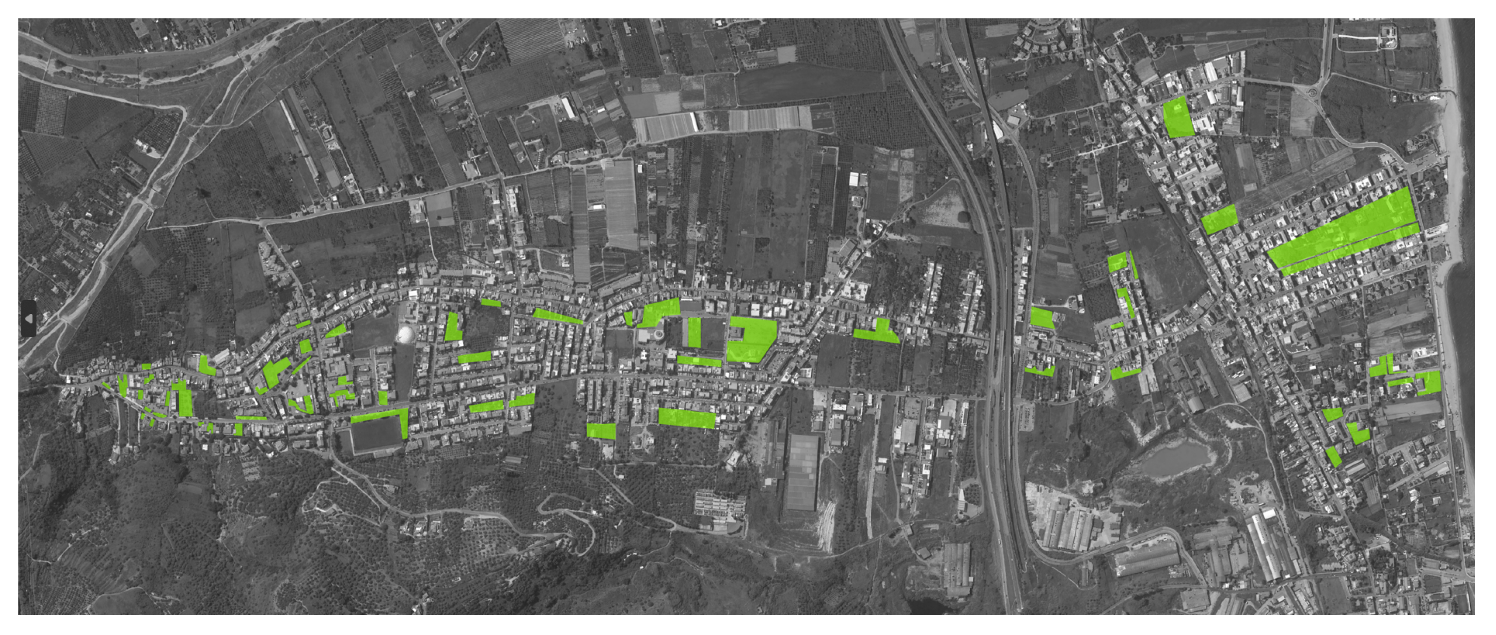
Figure 1.
Study area and localization of Torregrotta Town (adapted from https://earth.google.com/, accessed on 30 September 2022).
Figure 1.
Study area and localization of Torregrotta Town (adapted from https://earth.google.com/, accessed on 30 September 2022).

Figure 2.
Trends of the water flow rates in and out of the tank measured each 120 min [35].
Figure 2.
Trends of the water flow rates in and out of the tank measured each 120 min [35].

Figure 3.
Monthly water consumption obtained by the surveys in the period 1998–2018 [36].
Figure 3.
Monthly water consumption obtained by the surveys in the period 1998–2018 [36].

Figure 4.
Temperature data in the period 1998–2018 (Hydrological Annals, Regione Sicilia [37], http://www.sias.regione.sicilia.it, accessed on 30 September 2022).
Figure 4.
Temperature data in the period 1998–2018 (Hydrological Annals, Regione Sicilia [37], http://www.sias.regione.sicilia.it, accessed on 30 September 2022).

Figure 5.
Users obtained by the surveys in the period 1998–2018.

Figure 6.
Rainy day monthly surveys in the period 1998–2018.

Figure 7.
Correlation matrix of parameters and volume consumption.

Figure 8.
Comparison of the performance between the predicted and training data.

Figure 9.
The total garden area supplied by the hydraulic system.

Figure 10.
Typical trend of annual water consumption.

Figure 11.
Comparison of rainy days provided by the hydrological annals and the estimate provided by the Copernicus toolbox.
Figure 11.
Comparison of rainy days provided by the hydrological annals and the estimate provided by the Copernicus toolbox.

Figure 12.
Comparison of temperature provided by the hydrological annals and the estimate provided by the Copernicus toolbox.
Figure 12.
Comparison of temperature provided by the hydrological annals and the estimate provided by the Copernicus toolbox.

Figure 13.
Comparison of rainy days provided by the hydrological annals and the calibrated estimate provided by the Copernicus toolbox.
Figure 13.
Comparison of rainy days provided by the hydrological annals and the calibrated estimate provided by the Copernicus toolbox.

Figure 14.
Comparison of temperature provided by the hydrological annals and the calibrated estimate provided by the Copernicus toolbox.
Figure 14.
Comparison of temperature provided by the hydrological annals and the calibrated estimate provided by the Copernicus toolbox.

Figure 15.
Future forecast—rainy days.

Figure 16.
Future forecast—temperature.

Figure 17.
Comparison between the adaptive function and the observed rainy days. The values are normalized with respect to the minimum and maximum values as found in Equation (7).
Figure 17.
Comparison between the adaptive function and the observed rainy days. The values are normalized with respect to the minimum and maximum values as found in Equation (7).

Figure 18.
Comparison between the adaptive function and the observed temperature. The values are normalized with respect to the minimum and maximum values as found in Equation (7).
Figure 18.
Comparison between the adaptive function and the observed temperature. The values are normalized with respect to the minimum and maximum values as found in Equation (7).

Figure 19.
Comparison between the adaptive function and the observed users. The values are normalized with respect to the minimum and maximum values as found in Equation (7).
Figure 19.
Comparison between the adaptive function and the observed users. The values are normalized with respect to the minimum and maximum values as found in Equation (7).

Figure 20.
Observed and future water consumption up to 2028. The future trend was obtained by applying the trained ANN.
Figure 20.
Observed and future water consumption up to 2028. The future trend was obtained by applying the trained ANN.

Figure 21.
Graphical representation of function (9).
Figure 21.
Graphical representation of function (9).

Figure 22.
Application of function (12) to recover hourly volumes.
Figure 22.
Application of function (12) to recover hourly volumes.

Figure 23.
Random function (14) applied to the water flow rate within the tank.
Figure 23.
Random function (14) applied to the water flow rate within the tank.

Figure 24.
Volume trend in m3 in hours. Red circle denotes crisis event.

Figure 25.
Reduction in the hours of crisis as a function of the adopted volume of the reservoir.


Table 1.
Performance of the ANN model for different architectures.
| Numbers of Neurons | Data Training | Data Testing | ||||
|---|---|---|---|---|---|---|
| r | m3 | r | m3 | |||
| 5 | 0.824 | 1423.20 | 0.732 | 0.798 | 1501.80 | 0.694 |
| 8 | 0.931 | 1364.22 | 0.821 | 0.907 | 1411.82 | 0.817 |
| 13 | 0.961 | 1234.50 | 0.920 | 0.947 | 1253.78 | 0.947 |
| 15 | 0.908 | 1345.10 | 0.897 | 0.929 | 1378.90 | 0.881 |
Table 2.
Performance of the ANN model.
| Max Iteration | Data Training | Data Testing | ||||
|---|---|---|---|---|---|---|
| r | m3 | r | m3 | |||
| 2000 | 0.961 | 1234.50 | 0.920 | 0.947 | 1253.78 | 0.947 |
Disclaimer/Publisher’s Note: The statements, opinions and data contained in all publications are solely those of the individual author(s) and contributor(s) and not of MDPI and/or the editor(s). MDPI and/or the editor(s) disclaim responsibility for any injury to people or property resulting from any ideas, methods, instructions or products referred to in the content. |
© 2023 by the authors. Licensee MDPI, Basel, Switzerland. This article is an open access article distributed under the terms and conditions of the Creative Commons Attribution (CC BY) license (https://creativecommons.org/licenses/by/4.0/).
Share and Cite
MDPI and ACS Style
Saya, B.; Faraci, C. Application of Artificial Neural Networks for Predicting Small Urban-Reservoir Volumes: The Case of Torregrotta Town (Italy). Water 2023, 15, 1747. https://doi.org/10.3390/w15091747
AMA Style
Saya B, Faraci C. Application of Artificial Neural Networks for Predicting Small Urban-Reservoir Volumes: The Case of Torregrotta Town (Italy). Water. 2023; 15(9):1747. https://doi.org/10.3390/w15091747
Chicago/Turabian StyleSaya, Biagio, and Carla Faraci. 2023. "Application of Artificial Neural Networks for Predicting Small Urban-Reservoir Volumes: The Case of Torregrotta Town (Italy)" Water 15, no. 9: 1747. https://doi.org/10.3390/w15091747
Note that from the first issue of 2016, this journal uses article numbers instead of page numbers. See further details here.