
Understanding the Climate Change and Land Use Impact on Streamflow in the Present and Future under CMIP6 Climate Scenarios for the Parvara Mula Basin, India


Abstract
:1. Introduction
2. Study Area and Data Collection
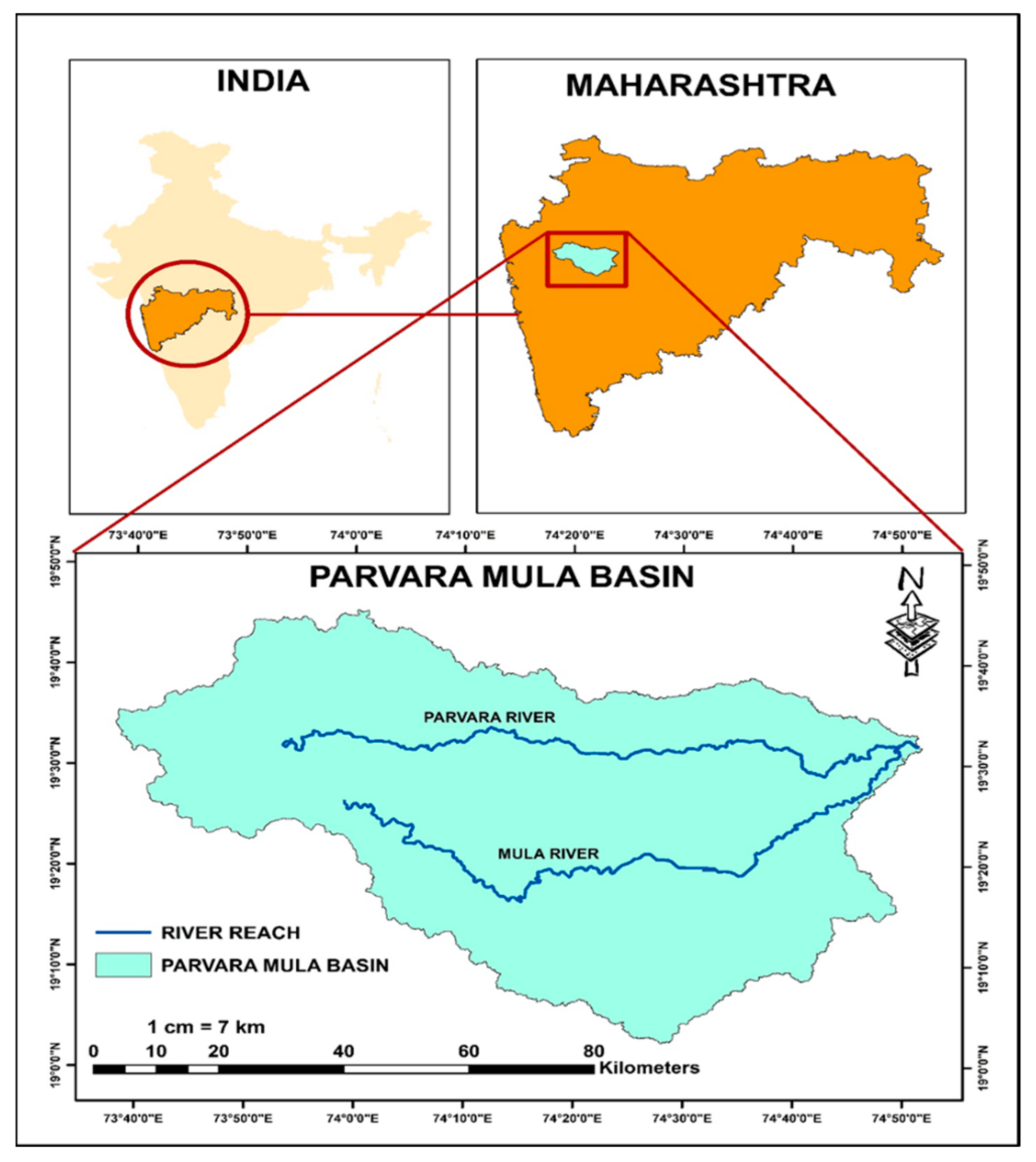
2.1. Study Area
2.2. Data Collection
2.2.1. Hydro-Meteorological Data
2.2.2. GCM Data
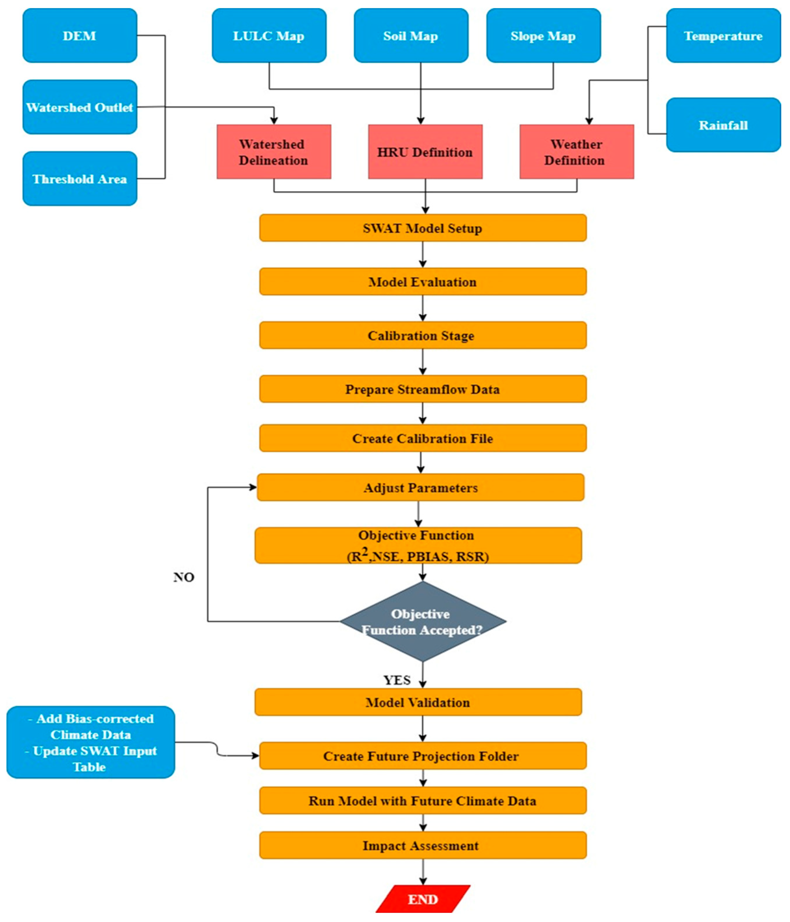
3. Methodology
- Collect and sort meteorological and hydrological data.
- Preparation of input maps such as DEM, soil, slope, and LULC.
- Watershed delineation using DEM involves fixing the basin outlet and setting a threshold area.
- HRU generation by overlaying the LULC, soil, and slope maps.
- Setting up the SWAT model with the input data.
- Evaluating the model and obtaining the output data.
- Calibrating the model using the SUFI-2 algorithm by finding the sensitive parameter.
- Checking the model’s performance for the calibration period; if okay, validating the model, or else adjusting the parameters again.
- Validation of the model under the fitted parameter values obtained during the calibration.
- Updating the SWAT model with future climatic data.
- Simulating the model with the future climatic data for impact assessment.
3.1. SWAT Model Setup
3.1.1. Watershed Delineation
3.1.2. Digital Elevation Model (DEM)
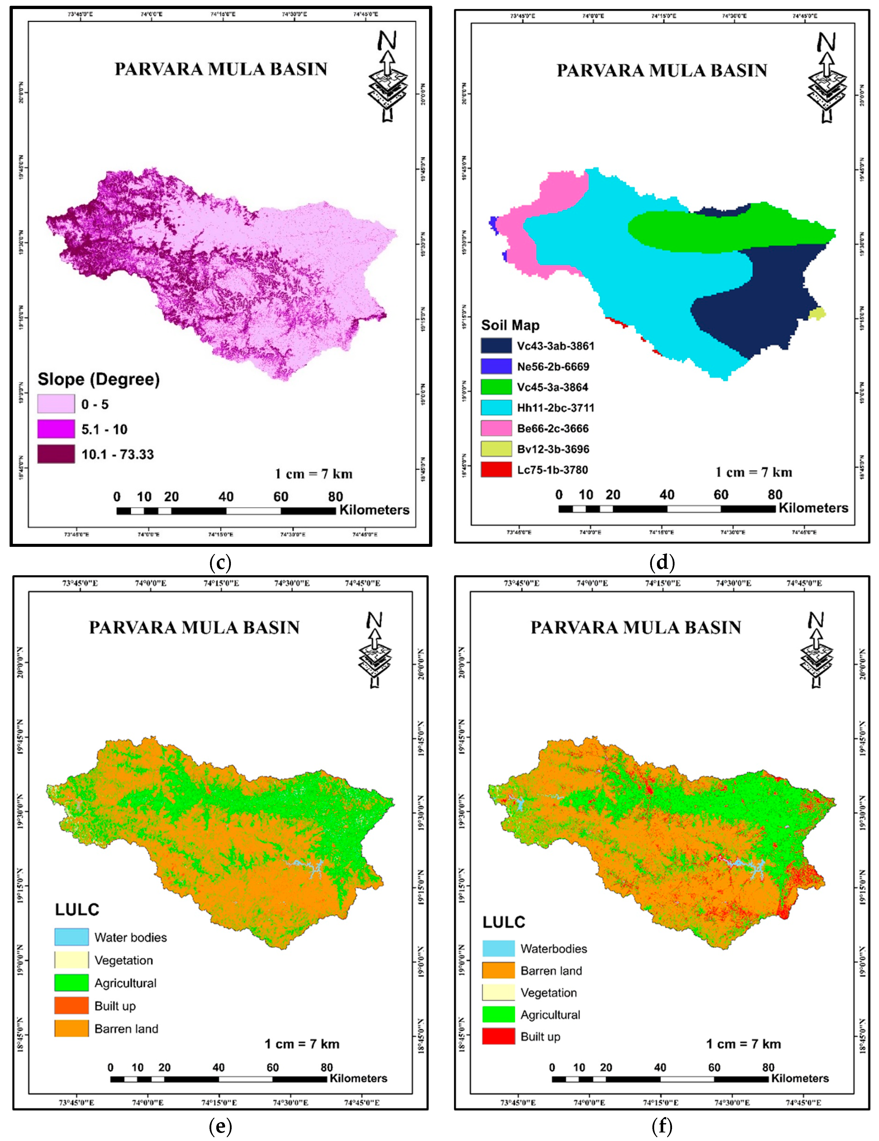
3.1.3. Slope Map
3.1.4. Soil Map
3.1.5. Land Use Land Cover
3.1.6. Climate Data
3.1.7. Hydrologic Response Unit (HRU) Generation
3.2. Model Simulation, Calibration, and Validation
3.2.1. SWAT Simulation
3.2.2. SWAT Calibration and Uncertainty Analysis Program (SWAT-CUP)
3.2.3. Sensitivity Analysis
3.2.4. Model Calibration
3.2.5. Model Validation
3.3. Model Performance Criteria
- Coefficient of determination (R2): (R2) calculates the correlation value between measured and estimated values by comparing the combined scattering of the measured and estimated series to the single scattering. Its value ranges between zero and one. The correlation between the observed and estimated SF can be understood with the value of (R2). Low correlation is described with a value close to zero, whereas a high correlation is indicated by a value to close to one.
- Nash–Sutcliffe efficiency (NSE): It is among the most extensively used hydrological model statistical measures. Its value varies from infinity to one, with one representing a perfect model. As the value approaches zero, the performance of the model degrades.
- Percent bias (PBIAS): PBIAS shows the mean tendency of simulated outcome to be smaller or larger than the observed data. Its optimal value is zero. A positive PBIAS value means the model is an underprediction of the results, whereas a negative value suggests overprediction.
- Ratio of root-mean-square error to measured standard deviation (RSR): RSR is selected as a complimentary statistical metric to RMSE. The optimal value of RSR is zero. However, the higher the RSR, the lower the performance of the model.
- Estimating p-factor: Curve Number (CN) Method: This method is based on the relationship between the antecedent moisture condition and the amount of rainfall that becomes runoff. The CN value is calculated using soil type, land use, and hydrologic soil group. Once the CN value is obtained, it is used to estimate the surface runoff using the SCS (Soil Conservation Service) equation.
- Estimating r-factor: Muskingum-Cunge Method: This method is based on the principle of flood routing and uses the Muskingum-Cunge equation to estimate the travel time and attenuation of flood waves. The equation requires input parameters such as channel length, channel slope, and channel roughness.

| Performance | RSR | NSE | PBIAS |
|---|---|---|---|
| Very Good | 0 ≤ RSR ≤ 0.5 | 0.75 < NSE ≤ 1 | PBIAS < ± 10 |
| Good | 0.5 ≤ RSR ≤ 0.6 | 0.65 < NSE ≤ 0.75 | ± 10 ≤ PBIAS < ± 15 |
| Satisfactory | 0.6 ≤ RSR ≤ 0.7 | 0.50 < NSE ≤ 0.65 | ± 15 ≤ PBIAS < ± 25 |
| Unsatisfactory | RSR > 0.7 | NSE ≤ 0.50 | PBIAS ≥ ± 25 |
4. Results and Discussion
4.1. LULC Accuracy Assessment Using Kappa Analysis
Accuracy Assessment of LULC Map (2010) and LULC Map (2018)
4.2. Sensitivity Analysis Using SUFI-2
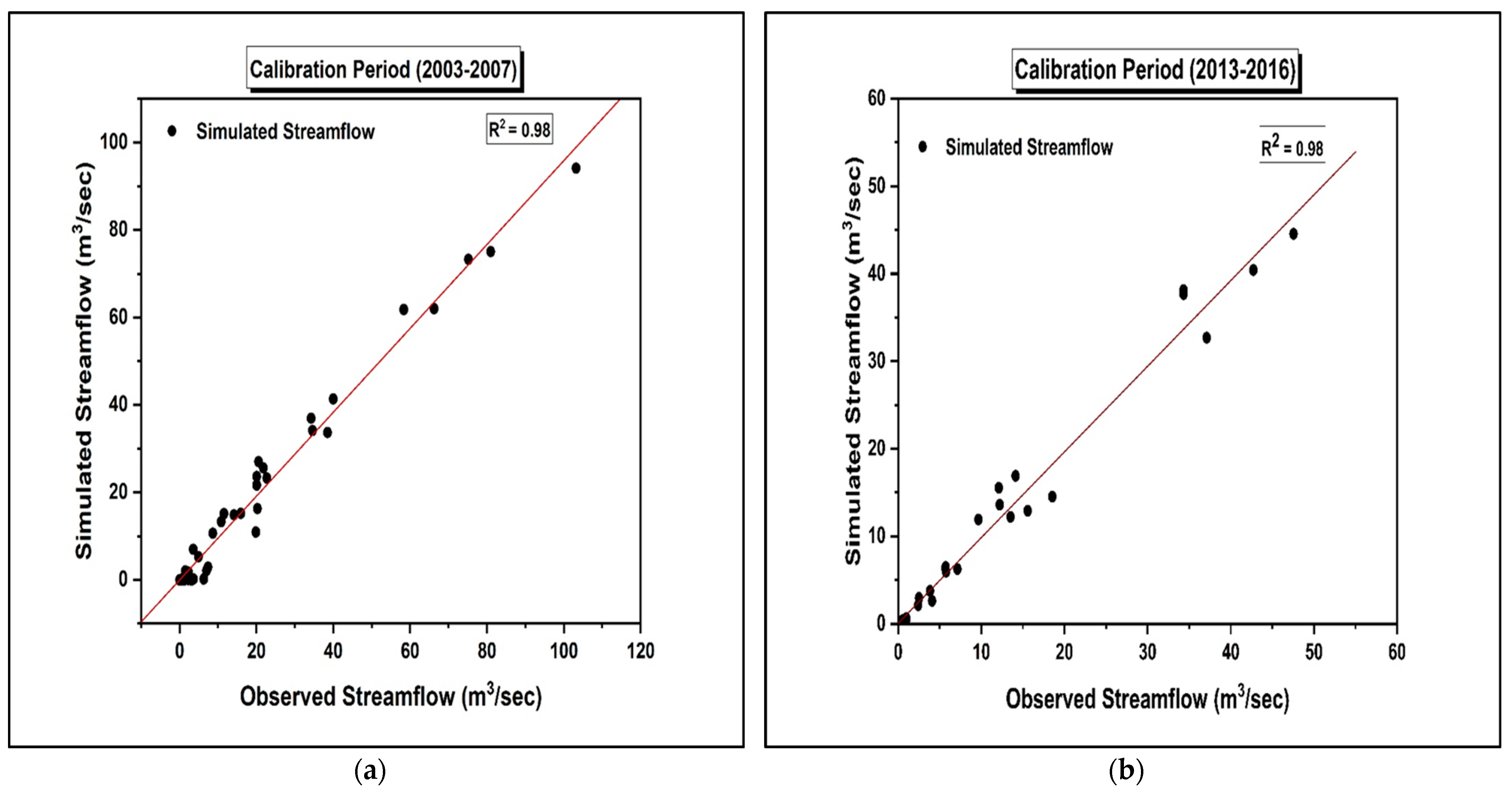
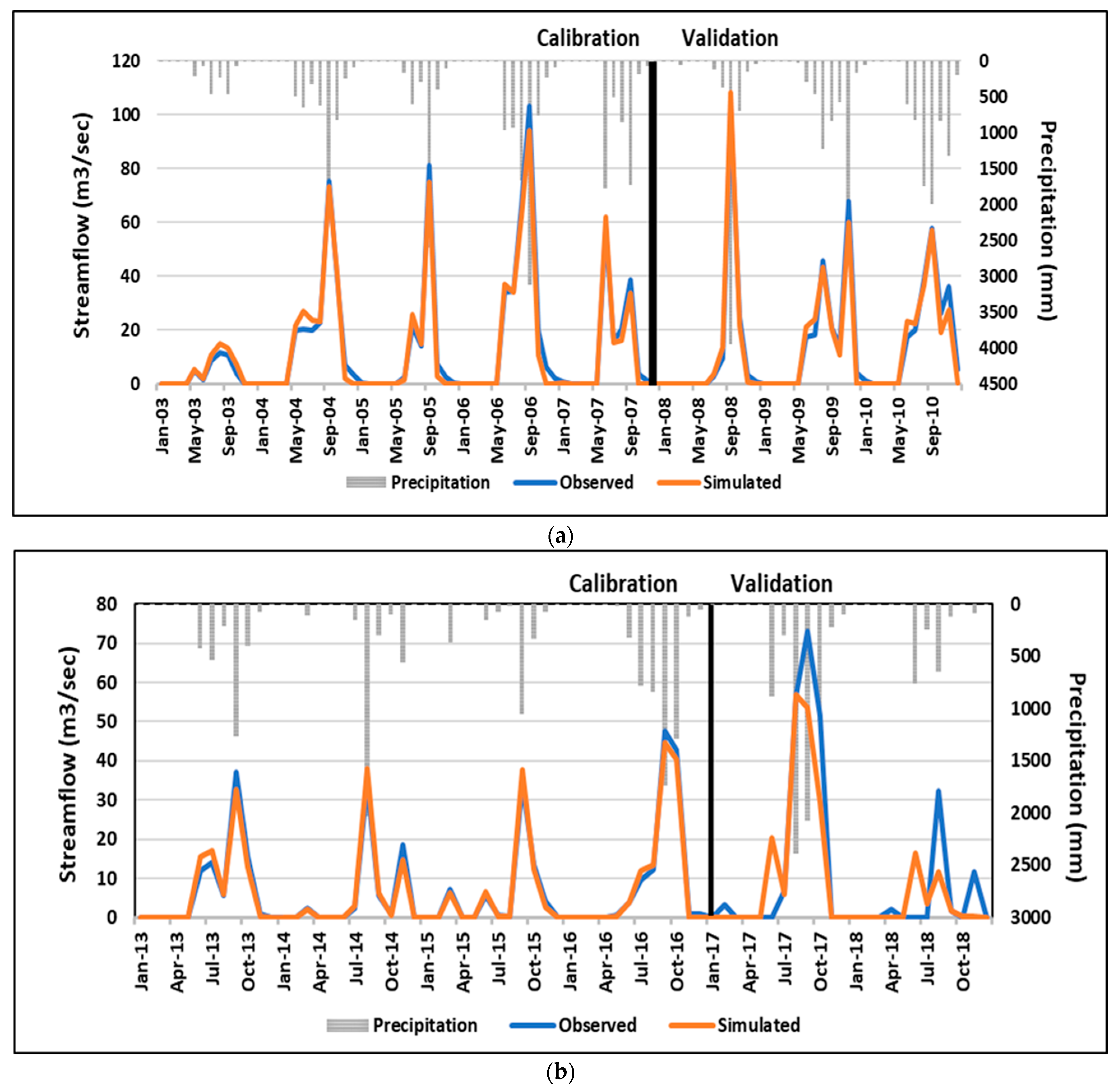
4.3. Model Calibration
4.4. Model Validation
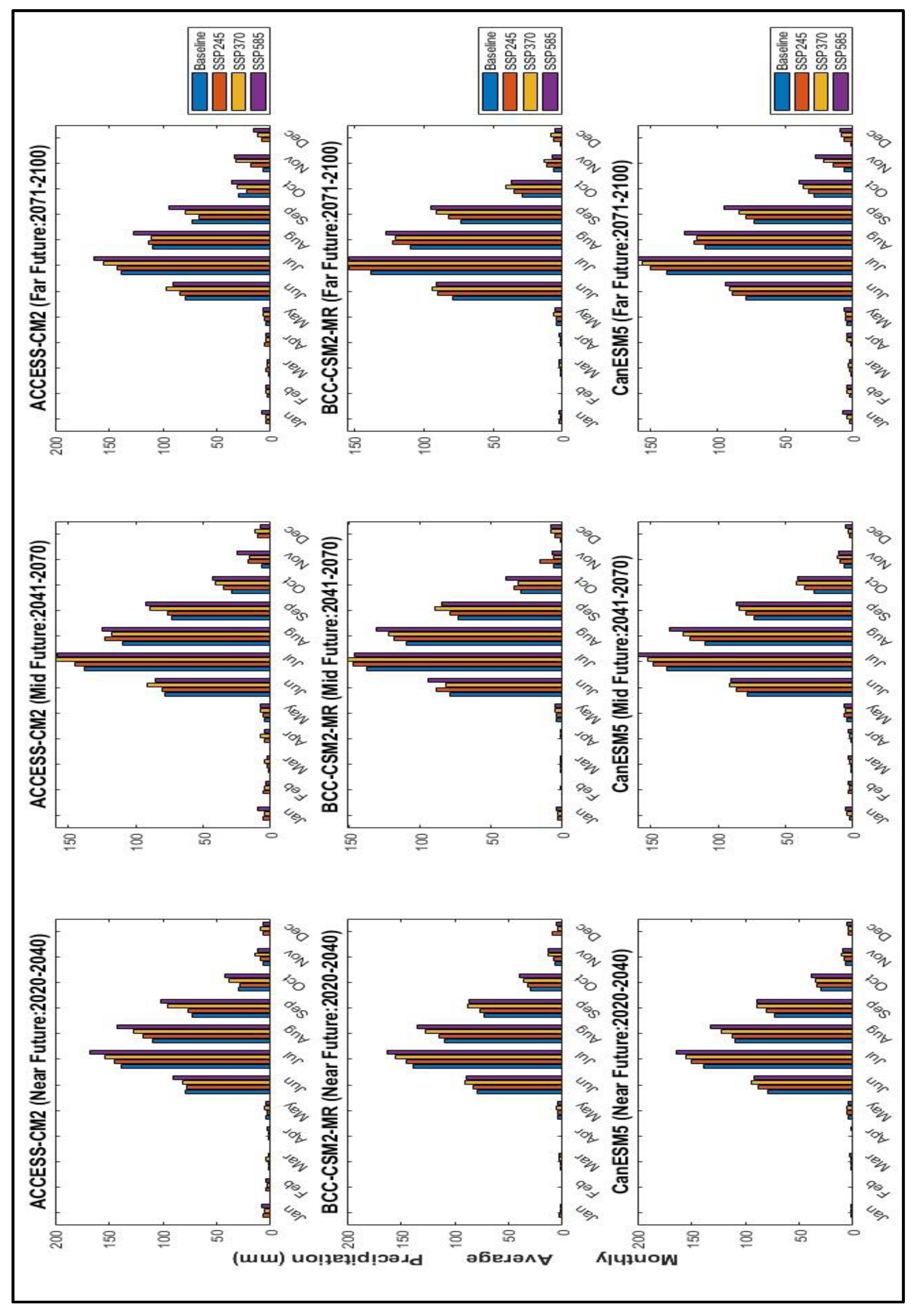
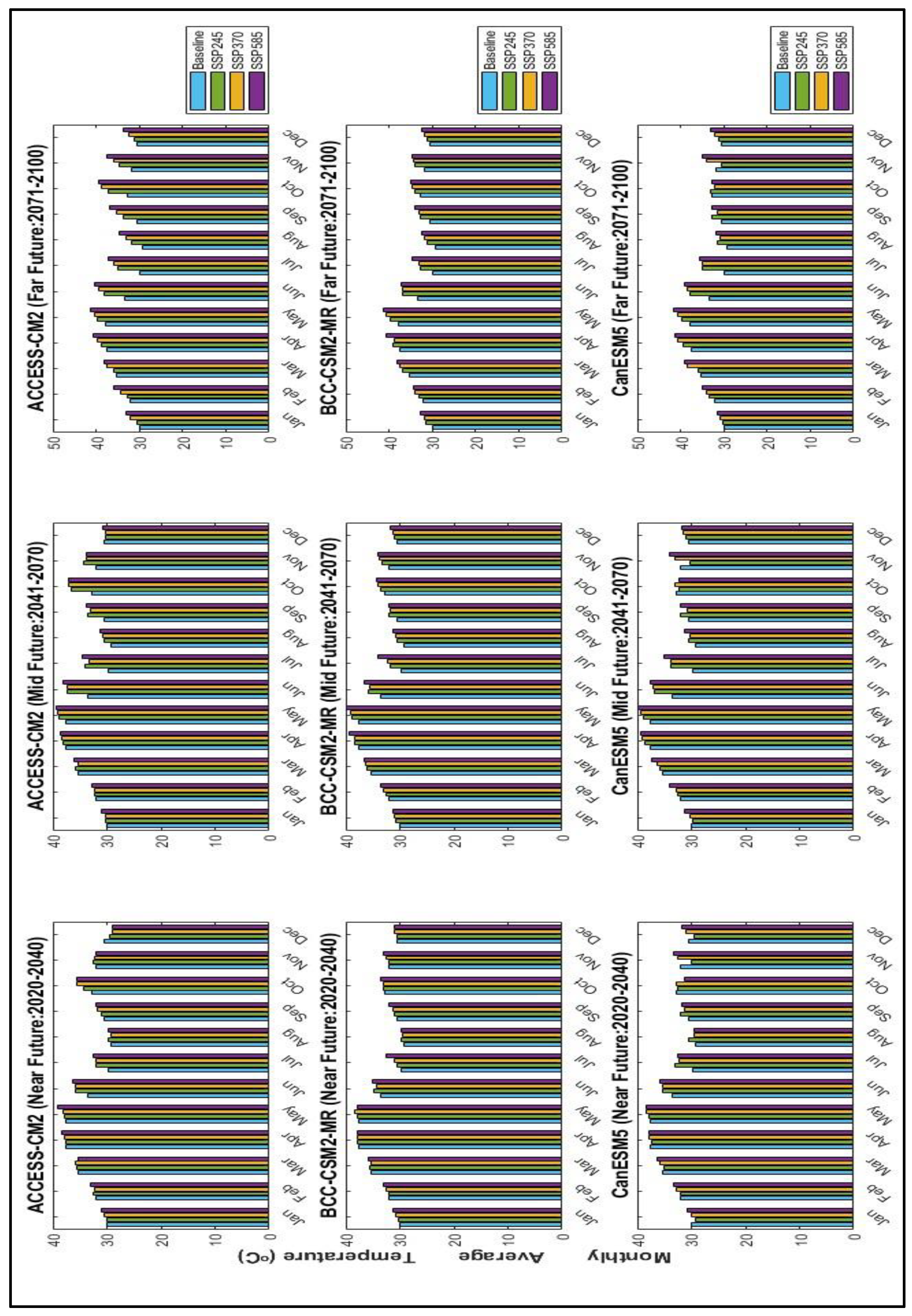
4.5. Projected Changes in Precipitation and Temperature for the Future Period (2020–2100)
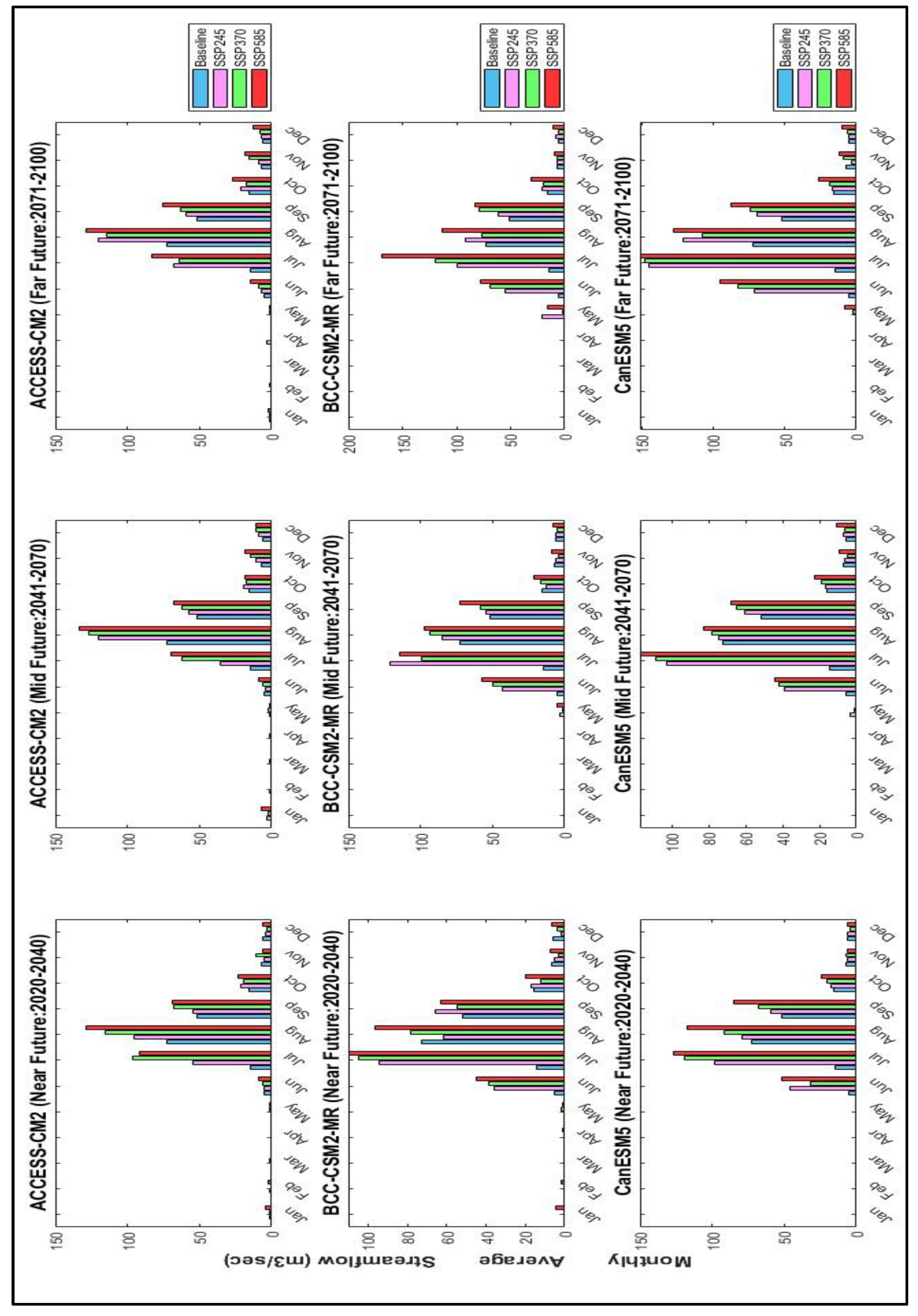
4.6. Projected Changes in Streamflow for the Future Period (2020–2100)
4.6.1. Projected Changes in Streamflow under ACCESS-CM2
4.6.2. Projected Changes in Streamflow under BCC-CSM2-MR
4.6.3. Projected Changes in Streamflow under CanESM5
4.7. Mean Ensembled Model for Future Scenarios under Near Future (2020–2040), Mid Future (2041–2070), and Far Future (2071–2100) Time Horizons
5. Discussion
6. Conclusions
Supplementary Materials
Author Contributions
Funding
Institutional Review Board Statement
Data Availability Statement
Conflicts of Interest
Abbreviations
| CC | climate change |
| LULC | Land Use Land Cover |
| WR | water resources |
| SF | streamflow |
| PMB | Parvara Mula Basin |
| SWAT | Soil and Water Assessment Tool |
| CUP | Calibration Uncertainty Program |
| R2 | Correlation determination |
| NSE | Nash-Sutcliffe efficiency |
| PBIAS | Percentage bias |
| RSR | Ratio of root-mean-square error to measured standard deviation |
| CMIP6 | Coupled Model Inter-Comparison Project Phase 6 |
| GCM | Global climate models |
| CM | Climate model |
| CanESM5 | Canadian Earth System Model version 5 |
| BCC | CSM2 |
| MR | Beijing Climate Center (BCC) Climate System Model |
| ff | far future |
| nf | near future |
| mf | mid future |
| DEM | digital elevation model |
| IMD | India Meteorological Department |
| SUFI-2 | Sequential Uncertainty Fitting version 2 |
| SCS | Soil Conservation Services |
| WGS | World Geodetic System |
| UTM | Universal Transverse Mercator |
| HRU | Hydrologic Response Unit |
| FAO | Food and Agriculture Organization |
| GIS | Geographic Information System |
| SA | sensitivity analysis (SA). |
| LSA | local sensitivity (LSA) |
| GSA | global sensitivity (GSA). |
| USGS | United States Geological Survey |
References
- Huang, J.; Ji, M.; Xie, Y.; Wang, S.; He, Y.; Ran, J. Global semi-arid climate change over last 60 years. Clim. Dyn. 2015, 46, 1131–1150. [Google Scholar] [CrossRef]
- Schwinning, S.; Sala, O.; Loik, M.E.; Ehleringer, J.R. Thresholds, memory, and seasonality: Understanding pulse dynamics in arid/semi-arid ecosystems. Oecologia 2004, 141, 191–193. [Google Scholar] [CrossRef]
- Abbas, S.; Dastgeer, G. Analysing the impacts of climate variability on the yield of Kharif rice over Punjab, Pakistan. Nat. Resour. Forum 2021, 45, 329–349. [Google Scholar] [CrossRef]
- Li, C.; Zwiers, F.; Zhang, X.; Li, G.; Sun, Y.; Wehner, M. Changes in Annual Extremes of Daily Temperature and Precipitation in CMIP6 Models. J. Clim. 2021, 34, 3441–3460. [Google Scholar] [CrossRef]
- Yaseen, M.; Waseem, M.; Latif, Y.; Azam, M.I.; Ahmad, I.; Abbas, S.; Sarwar, M.K.; Nabi, G. Statistical Downscaling and Hydrological Modeling-Based Runoff Simulation in Trans-Boundary Mangla Watershed Pakistan. Water 2020, 12, 3254. [Google Scholar] [CrossRef]
- Paul, S.; Ghosh, S.; Oglesby, R.; Pathak, A.; Chandrasekharan, A.; Ramsankaran, R. Weakening of Indian Summer Monsoon Rainfall due to Changes in Land Use Land Cover. Sci. Rep. 2016, 6, 32177. [Google Scholar] [CrossRef] [PubMed]
- Saharwardi, S.; Mahadeo, A.S.; Kumar, P. Understanding drought dynamics and variability over Bundelkhand region. J. Earth Syst. Sci. 2021, 130, 1–16. [Google Scholar] [CrossRef]
- Sharmila, S.; Joseph, S.; Sahai, A.; Abhilash, S.; Chattopadhyay, R. Future projection of Indian summer monsoon variability under climate change scenario: An assessment from CMIP5 climate models. Glob. Planet. Chang. 2015, 124, 62–78. [Google Scholar] [CrossRef]
- Wagner, P.D.; Bhallamudi, S.M.; Narasimhan, B.; Kantakumar, L.N.; Sudheer, K.; Kumar, S.; Schneider, K.; Fiener, P. Dynamic integration of land use changes in a hydrologic assessment of a rapidly developing Indian catchment. Sci. Total Environ. 2015, 539, 153–164. [Google Scholar] [CrossRef]
- Chanapathi, T.; Thatikonda, S. Investigating the impact of climate and land-use land cover changes on hydrological predictions over the Krishna river basin under present and future scenarios. Sci. Total Environ. 2020, 721, 137736. [Google Scholar] [CrossRef] [PubMed]
- Vandana, K.; Islam, A.; Sarthi, P.P.; Sikka, A.K.; Kapil, H. Assessment of potential impact of climate change on streamflow: A case study of the Brahmani River basin, India. J. Water Clim. Chang. 2018, 10, 624–641. [Google Scholar] [CrossRef]
- Kundzewicz, Z.W.; Robson, A. Change detection in hydrological records—A review of the methodology / Revue méthodologique de la détection de changements dans les chroniques hydrologiques. Hydrol. Sci. J. 2004, 49, 7–19. [Google Scholar] [CrossRef]
- IPCC. Intergovernmental Panel on Climate Change, Managing the Risks of Extreme Events and Disasters to Advance Climate Change Adaptation: Special Report of the Intergovernmental Panel on Climate Change; Cambridge University Press: New York, NY, USA, 2012. [Google Scholar]
- IPCC. Climate Change 2014 : Impacts, Adaptation, and Vulnerability: Working Group II Contribution to the Fifth Assessment Report of the Intergovernmental Panel on Climate Change; Cambridge University Press: New York, NY, USA, 2014. [Google Scholar]
- Mendoza, P.A.; Clark, M.P.; Mizukami, N.; Newman, A.J.; Barlage, M.; Gutmann, E.D.; Rasmussen, R.M.; Rajagopalan, B.; Brekke, L.D.; Arnold, J.R. Effects of Hydrologic Model Choice and Calibration on the Portrayal of Climate Change Impacts. J. Hydrometeorol. 2015, 16, 762–780. [Google Scholar] [CrossRef]
- Sood, A.; Muthuwatta, L.; McCartney, M. A SWAT evaluation of the effect of climate change on the hydrology of the Volta River basin. Water Int. 2013, 38, 297–311. [Google Scholar] [CrossRef]
- Al-Mukhtar, M.; Dunger, V.; Merkel, B. Assessing the Impacts of Climate Change on Hydrology of the Upper Reach of the Spree River: Germany. Water Resour. Manag. 2014, 28, 2731–2749. [Google Scholar] [CrossRef]
- Jajarmizadeh, M.; Lafdani, E.K.; Harun, S.; Ahmadi, A. Application of SVM and SWAT models for monthly streamflow prediction, a case study in South of Iran. KSCE J. Civ. Eng. 2014, 19, 345–357. [Google Scholar] [CrossRef]
- Narsimlu, B.; Gosain, A.K.; Chahar, B.R. Assessment of Future Climate Change Impacts on Water Resources of Upper Sind River Basin, India Using SWAT Model. Water Resour. Manag. 2013, 27, 3647–3662. [Google Scholar] [CrossRef]
- Swain, S.S.; Mishra, A.; Sahoo, B.; Chatterjee, C. Water scarcity-risk assessment in data-scarce river basins under decadal climate change using a hydrological modelling approach. J. Hydrol. 2020, 590, 125260. [Google Scholar] [CrossRef]
- Kundu, S.; Khare, D.; Mondal, A. Past, present and future land use changes and their impact on water balance. J. Environ. Manag. 2017, 197, 582–596. [Google Scholar] [CrossRef]
- Hengade, N.; Eldho, T. I Assessment of LULC and climate change on the hydrology of Ashti Catchment, India using VIC model. J. Earth Syst. Sci. 2016, 125, 1623–1634. [Google Scholar] [CrossRef]
- Desai, S.; Singh, D.K.; Islam, A.; Sarangi, A. Impact of climate change on the hydrology of a semi-arid river basin of India under hypothetical and projected climate change scenarios. J. Water Clim. Chang. 2020, 12, 969–996. [Google Scholar] [CrossRef]
- Wang, B.; Zheng, L.; Liu, D.L.; Ji, F.; Clark, A.; Yu, Q. Using multi-model ensembles of CMIP5 global climate models to reproduce observed monthly rainfall and temperature with machine learning methods in Australia. Int. J. Clim. 2018, 38, 4891–4902. [Google Scholar] [CrossRef]
- Ahmed, K.; Sachindra, D.A.; Shahid, S.; Demirel, M.C.; Chung, E.-S. Selection of multi-model ensemble of general circulation models for the simulation of precipitation and maximum and minimum temperature based on spatial assessment metrics. Hydrol. Earth Syst. Sci. 2019, 23, 4803–4824. [Google Scholar] [CrossRef]
- Deb, P.; Babel, M.S.; Denis, A.F. Multi-GCMs approach for assessing climate change impact on water resources in Thailand. Model. Earth Syst. Environ. 2018, 4, 825–839. [Google Scholar] [CrossRef]
- Saraf, V.R.; Regulwar, D.G. Assessment of Climate Change for Precipitation and Temperature Using Statistical Downscaling Methods in Upper Godavari River Basin, India. J. Water Resour. Prot. 2016, 08, 31–45. [Google Scholar] [CrossRef]
- Roxy, M.K.; Ghosh, S.; Pathak, A.; Athulya, R.; Mujumdar, M.; Murtugudde, R.; Terray, P.; Rajeevan, M. A threefold rise in widespread extreme rain events over central India. Nat. Commun. 2017, 8, 708. [Google Scholar] [CrossRef]
- Aadhar, S.; Mishra, V. On the Projected Decline in Droughts Over South Asia in CMIP6 Multimodel Ensemble. J. Geophys. Res. Atmos. 2020, 125, e2020JD033587. [Google Scholar] [CrossRef]
- Anand, J.; Gosain, A.; Khosa, R. Prediction of land use changes based on Land Change Modeler and attribution of changes in the water balance of Ganga basin to land use change using the SWAT model. Sci. Total Environ. 2018, 644, 503–519. [Google Scholar] [CrossRef]
- Deepthi, B.; Sivakumar, B. General circulation models for rainfall simulations: Performance assessment using complex networks. Atmos. Res. 2022, 278, 106333. [Google Scholar] [CrossRef]
- Dixit, S.; Atla, B.M.; Jayakumar, K.V. Evolution and drought hazard mapping of future meteorological and hydrological droughts using CMIP6 model. Stoch. Environ. Res. Risk Assess. 2022, 36, 3857–3874. [Google Scholar] [CrossRef]
- Abbaspour, K.C.; Johnson, C.A.; Van Genuchten, M.T. Estimating uncertain flow and transport parameters using a sequential uncertainty fitting procedure. Vadose Zone J. 2004, 3, 1340–1352. [Google Scholar] [CrossRef]
- Sharifi, A.; Lang, M.W.; McCarty, G.W.; Sadeghi, A.M.; Lee, S.; Yen, H.; Rabenhorst, M.C.; Jeong, J.; Yeo, I.-Y. Improving model prediction reliability through enhanced representation of wetland soil processes and constrained model auto calibration—A paired watershed study. J. Hydrol. 2016, 541, 1088–1103. [Google Scholar] [CrossRef]
- Park, J.-Y.; Park, M.-J.; Ahn, S.-R.; Park, G.-A.; Yi, J.-E.; Kim, G.-S.; Srinivasan, R.; Kim, S.-J. Assessment of Future Climate Change Impacts on Water Quantity and Quality for a Mountainous Dam Watershed Using SWAT. Trans. ASABE 2011, 54, 1725–1737. [Google Scholar] [CrossRef]
- Shrestha, S.; Shrestha, M.; Shrestha, P.K. Evaluation of the swat model performance for simulating river discharge in the himalayan and tropical basins of asia. Hydrol. Res. 2018, 49, 846–860. [Google Scholar] [CrossRef]
- Mohseni, U.; Muskula, S.B. Rainfall-Runoff Modeling Using Artificial Neural Network—A Case Study of Purna Sub-Catchment of Upper Tapi Basin, India. Environ. Sci. Proc. 2023, 25, 1. [Google Scholar] [CrossRef]
- Moriasi, D.N.; Gitau, M.W.; Pai, N.; Daggupati, P. Hydrologic and Water Quality Models: Performance Measures and Evaluation Criteria. Trans. ASABE 2015, 58, 1763–1785. [Google Scholar] [CrossRef]
- Rwanga, S.S.; Ndambuki, J.M. Accuracy Assessment of Land Use/Land Cover Classification Using Remote Sensing and GIS. Int. J. Geosci. 2017, 8, 611–622. [Google Scholar] [CrossRef]
- Akhavan, S.; Abedi-Koupai, J.; Mousavi, S.-F.; Afyuni, M.; Eslamian, S.-S.; Abbaspour, K.C. Application of SWAT model to investigate nitrate leaching in Hamadan–Bahar Watershed, Iran. Agric. Ecosyst. Environ. 2010, 139, 675–688. [Google Scholar] [CrossRef]
- Chaemiso, S.E.; Abebe, A.; Pingale, S.M. Assessment of the impact of climate change on surface hydrological processes using SWAT: A case study of Omo-Gibe river basin, Ethiopia. Model. Earth Syst. Environ. 2016, 2, 1–15. [Google Scholar] [CrossRef]
- Asl-Rousta, B.; Mousavi, S.J.; Ehtiat, M.; Ahmadi, M. SWAT-Based Hydrological Modelling Using Model Selection Criteria. Water Resour. Manag. 2018, 32, 2181–2197. [Google Scholar] [CrossRef]
- Bennour, A.; Jia, L.; Menenti, M.; Zheng, C.; Zeng, Y.; Barnieh, B.A.; Jiang, M. Calibration and Validation of SWAT Model by Using Hydrological Remote Sensing Observables in the Lake Chad Basin. Remote Sens. 2022, 14, 1511. [Google Scholar] [CrossRef]
- Li, M.; Di, Z.; Duan, Q. Effect of sensitivity analysis on parameter optimization: Case study based on streamflow simulations using the SWAT model in China. J. Hydrol. 2021, 603, 126896. [Google Scholar] [CrossRef]
- Nilawar, A.P.; Waikar, M.L. Use of SWAT to determine the effects of climate and land use changes on streamflow and sediment concentration in the Purna River basin, India. Environ. Earth Sci. 2018, 77, 783. [Google Scholar] [CrossRef]
- Biswas, B.; Jadhav, R.S.; Tikone, N. Rainfall Distribution and Trend Analysis for Upper Godavari Basin, India, from 100 Years Record (1911–2010). J. Indian Soc. Remote Sens. 2019, 47, 1781–1792. [Google Scholar] [CrossRef]
- Senent-Aparicio, J.; Pérez-Sánchez, J.; Carrillo-García, J.; Soto, J. Using SWAT and Fuzzy TOPSIS to Assess the Impact of Climate Change in the Headwaters of the Segura River Basin (SE Spain). Water 2017, 9, 149. [Google Scholar] [CrossRef]
- Chunn, D.; Faramarzi, M.; Smerdon, B.; Alessi, D.S. Application of an Integrated SWAT–MODFLOW Model to Evaluate Potential Impacts of Climate Change and Water Withdrawals on Groundwater–Surface Water Interactions in West-Central Alberta. Water 2019, 11, 110. [Google Scholar] [CrossRef]
- Abdulahi, S.D.; Abate, B.; Harka, A.E.; Husen, S.B. Response of climate change impact on streamflow: The case of the Upper Awash sub-basin, Ethiopia. J. Water Clim. Chang. 2021, 13, 607–628. [Google Scholar] [CrossRef]
- Yang, M.; Li, Z.; Anjum, M.N.; Kayastha, R.; Kayastha, R.B.; Rai, M.; Zhang, X.; Xu, C. Projection of Streamflow Changes Under CMIP6 Scenarios in the Urumqi River Head Watershed, Tianshan Mountain, China. Front. Earth Sci. 2022, 10, 857854. [Google Scholar] [CrossRef]
- IPCC. Climate Change 2013: The Physical Science Basis. Contribution of Working Group I to the Fifth Assess-ment Report of the Intergovernmental Panel on Climate Change; Cambridge University Press: New York, NY, USA, 2013. [Google Scholar]
- Chawla, I.; Mujumdar, P.P. Isolating the impacts of land use and climate change on streamflow. Hydrol. Earth Syst. Sci. 2015, 19, 3633–3651. [Google Scholar] [CrossRef]
- Fang, G.H.; Yang, J.; Chen, Y.N.; Zammit, C. Comparing bias correction methods in downscaling meteorological variables for a hydrologic impact study in an arid area in China. Hydrol. Earth Syst. Sci. 2015, 19, 2547–2559. [Google Scholar] [CrossRef]
- Marchane, A.; Tramblay, Y.; Hanich, L.; Ruelland, D.; Jarlan, L. Climate change impacts on surface water resources in the Rheraya catchment (High Atlas, Morocco). Hydrol. Sci. J. 2017, 62, 979–995. [Google Scholar] [CrossRef]
- Luo, M.; Liu, T.; Meng, F.; Duan, Y.; Frankl, A.; Bao, A.; De Maeyer, P. Comparing Bias Correction Methods Used in Downscaling Precipitation and Temperature from Regional Climate Models: A Case Study from the Kaidu River Basin in Western China. Water 2018, 10, 1046. [Google Scholar] [CrossRef]
- Getahun, Y.S. Impact of Climate Change on Hydrology of the Upper Awash River Basin (Ethiopia): Inter-Comparison of Old SRES and New RCP Scenarios Assessing the Impact of Climate Change on the Hydrology of a Basin and Developing Adaptation Pathway. View Project. 2015. Available online: https://www.researchgate.net/publication/316505332 (accessed on 29 August 2022).
- Tibangayuka, N.; Mulungu, D.M.M.; Izdori, F. Assessing the potential impacts of climate change on streamflow in the data-scarce Upper Ruvu River watershed, Tanzania. J. Water Clim. Chang. 2022, 13, 3496–3513. [Google Scholar] [CrossRef]
- Tekleab, S.; Mohamed, Y.; Uhlenbrook, S. Hydro-climatic trends in the Abay/Upper Blue Nile basin, Ethiopia. Phys. Chem. Earth Parts A/B/C 2013, 61–62, 32–42. [Google Scholar] [CrossRef]
- Roba, N.T.; Kassa, A.K.; Geleta, D.Y. Modeling climate change impacts on crop water demand, middle Awash River basin, case study of Berehet woreda. Water Pract. Technol. 2021, 16, 864–885. [Google Scholar] [CrossRef]
- Gizaw, M.S.; Biftu, G.F.; Gan, T.Y.; Moges, S.A.; Koivusalo, H. Potential impact of climate change on streamflow of major Ethiopian rivers. Clim. Chang. 2017, 143, 371–383. [Google Scholar] [CrossRef]
- Tadese, M.T.; Kumar, L.; Koech, R.; Zemadim, B. Hydro-Climatic Variability: A Characterisation and Trend Study of the Awash River Basin, Ethiopia. Hydrology 2019, 6, 35. [Google Scholar] [CrossRef]
- Saraf, V.R.; Regulwar, D.G. Impact of Climate Change on Runoff Generation in the Upper Godavari River Basin, India. J. Hazard. Toxic Radioact. Waste 2018, 22, 04018021. [Google Scholar] [CrossRef]
- Sharannya, T.M.; Mudbhatkal, A.; Mahesha, A. Assessing climate change impacts on river hydrology—A case study in the Western Ghats of India. J. Earth Syst. Sci. 2018, 127, 78. [Google Scholar] [CrossRef]
- Ma, D.; Qian, B.; Gu, H.; Sun, Z.; Xu, Y. Assessing climate change impacts on streamflow and sediment load in the upstream of the Mekong River basin. Int. J. Clim. 2021, 41, 3391–3410. [Google Scholar] [CrossRef]


| Data | Resolution | Source |
|---|---|---|
| DEM | 30 m | https://earthexplorer.usgs.gov/ (accessed on 1 March 2023) |
| Soil Map | 1000 m | https://data.apps.fao.org/map/catalog/srv/eng/catalog.search (accessed on 1 March 2023) |
| Slope Map | 30 m | https://earthexplorer.usgs.gov/ (accessed on 1 March 2023) |
| LULC | 30 m | https://earthexplorer.usgs.gov/ (accessed on 1 March 2023) |
| Rainfall | 0.25 m | India Meteorological Department (IMD) |
| Temperature | 1° | India Meteorological Department (IMD) |
| Discharge | - | Central water Commission (CWC)–Krishna Godavari Basin Organization |
| LULC (2010) | LULC (2018) | ||||||
|---|---|---|---|---|---|---|---|
| Sr. No | Class | Area (km2) | % Area | Sr. No | Class | Area (km2) | % Area |
| 1 | Water Bodies | 32.42 | 0.97 | 1 | Water Bodies | 66.56 | 1.19 |
| 2 | Vegetation | 125.19 | 2.25 | 2 | Vegetation | 16.66 | 0.30 |
| 3 | Agricultural Land | 1895.73 | 34 | 3 | Agricultural Land | 2046.46 | 36.70 |
| 4 | Built-up Area | 165.81 | 2.97 | 4 | Built-up Area | 554.64 | 9.95 |
| 5 | Barren land | 3355.97 | 60.19 | 5 | Barren land | 2890.78 | 51.85 |
| Sr. No | GCM | Source |
|---|---|---|
| 1 | ACCESS-CM2 | Australian Community Climate and Earth System Simulator Coupled Model |
| 2 | BCC-CSM2-MR | Beijing Climate Centre Climate System Model |
| 3 | CanESM5 | Canadian Earth System Model |
| Sr. No | Kappa Coefficient | Agreement |
|---|---|---|
| 1 | <0 | Poor |
| 2 | 0–0.2 | Slight |
| 3 | 0.21–0.4 | Fair |
| 4 | 0.41–0.6 | Moderate |
| 5 | 0.61–0.8 | Substantial |
| 6 | 0.81–1.0 | Almost Perfect |
| LULC (2010) | Barren Land | Water Bodies | Built-Up Area | Vegetation | Agricultural Land | Total (User) |
| Barren Land | 18 | 0 | 1 | 1 | 0 | 20 |
| Water bodies | 1 | 18 | 0 | 0 | 1 | 20 |
| Built-Up Area | 6 | 0 | 10 | 4 | 0 | 20 |
| Vegetation | 2 | 0 | 0 | 16 | 2 | 20 |
| Agricultural Land | 0 | 0 | 0 | 4 | 16 | 20 |
| Total (producer) | 27 | 18 | 11 | 25 | 19 | 100 |
| LULU (2018) | Barren land | Water bodies | Built-Up Area | Vegetation | Agricultural Land | Total (user) |
| Barren Land | 19 | 0 | 0 | 1 | 0 | 20 |
| Water bodies | 1 | 19 | 0 | 0 | 0 | 20 |
| Built-Up Area | 5 | 0 | 11 | 4 | 0 | 20 |
| Vegetation | 2 | 0 | 0 | 18 | 0 | 20 |
| Agricultural Land | 0 | 0 | 0 | 4 | 16 | 20 |
| Total (producer) | 27 | 19 | 11 | 27 | 16 | 100 |
| Period (2003–2010) | Period (2013–2018) | ||||||
|---|---|---|---|---|---|---|---|
| Sr. No | Parameter | t Stat | p-Value | Sr. No | Parameter | t Stat | p-Value |
| 1 | R__CN2.mgt | 27.81852 | 0.000000 | 1 | R__CN2.mgt | 17.81852 | 0.000000 |
| 2 | V__GW_REVAP.gw | −1.11035 | 0.267024 | 2 | V__GW_REVAP.gw | 0.595071 | 0.551886 |
| 3 | V__ESCO.hru | 8.851582 | 0.000000 | 3 | V__ESCO.hru | 3.944408 | 0.000083 |
| 4 | V__CH_N2.rte | −2.73454 | 0.006320 | 4 | V__CH_N2.rte | 0.416615 | 0.677019 |
| 5 | R__SURLAG.bsn | 0.437570 | 0.661760 | 5 | R__SURLAG.bsn | 0.168647 | 0.866096 |
| 6 | R__CANMX.hru | 0.249366 | 0.803111 | 6 | R__CANMX.hru | 0.615628 | 0.538233 |
| 7 | R__SOL_AWC(..).sol | 0.217374 | 0.827946 | 7 | R__SOL_AWC(..).sol | 0.052711 | 0.957968 |
| Sr. No | Parameter | Calibration (2003–2007) | Validation (2008–2010) | Calibration (2013–2016) | Validation (2017–2018) |
|---|---|---|---|---|---|
| 1 | R2 | 0.98 | 0.98 | 0.98 | 0.81 |
| 2 | NSE | 0.98 | 0.98 | 0.98 | 0.79 |
| 3 | PBIAS | 4.3 | 4.1 | 1.1 | 16 |
| 4 | RSR | 0.13 | 0.15 | 0.13 | 0.46 |
| 5 | p-factor | 0.72 | 0.64 | 0.71 | 0.5 |
| 6 | r-factor | 0.19 | 0.21 | 0.44 | 0.16 |
| Average Annual Precipitation | |||||||||
| GCM | Near Future | Mid Future | Far Future | ||||||
| ssp245 | ssp370 | ssp585 | ssp245 | ssp370 | ssp585 | ssp245 | ssp370 | ssp585 | |
| ACCESS-CM2 | 8.19% | 19.24% | 21.52% | 14.57% | 22.27% | 27.00% | 14.95% | 24.36% | 30.00% |
| BCC-CSM2-MR | 8.04% | 18.71% | 22.03% | 12.09% | 20.73% | 26.57% | 15.47% | 23.41% | 27.37% |
| CanESM5 | 9.80% | 20.52% | 22.32% | 12.79% | 24.37% | 27.79% | 16.67% | 27.01% | 33.30% |
| Average Annual Temperature | |||||||||
| GCM | Near Future | Mid Future | Far Future | ||||||
| ssp245 | ssp370 | ssp585 | ssp245 | ssp370 | ssp585 | ssp245 | ssp370 | ssp585 | |
| ACCESS-CM2 | 0.57% | 5.32% | 7.48% | 0.79% | 5.14% | 11.41% | 1.28% | 6.56% | 14.86% |
| BCC-CSM2-MR | 1.08% | 3.53% | 5.71% | 1.59% | 4.26% | 7.09% | 2.84% | 6.02% | 9.56% |
| CanESM5 | 0.51% | 2.35% | 4.53% | 0.70% | 3.32% | 6.97% | 0.82% | 4.89% | 9.39% |
| Average Annual Streamflow | |||||||||
| GCM | Near Future | Mid Future | Far Future | ||||||
| ssp245 | ssp370 | ssp585 | ssp245 | ssp370 | ssp585 | ssp245 | ssp370 | ssp585 | |
| ACCESS-CM2 | 34.29% | 57.38% | 32.73% | 40.02% | 33.90% | 70.30% | 51.28% | 46.30% | 71.92% |
| BCC-CSM2-MR | 64.01% | 33.70% | 41.58% | 67.13% | 32.05% | 30.41% | 71.32% | 68.01% | 79.49% |
| CanESM5 | 69.88% | 71.13% | 77.62% | 82.18% | 72.05% | 72.76% | 64.62% | 60.71% | 71.34% |
| Ensemble Mean Model | 56.04% | 59.65% | 68.15% | 63.17% | 45.39% | 57.84% | 72.21% | 64.13% | 80.74% |
Disclaimer/Publisher’s Note: The statements, opinions and data contained in all publications are solely those of the individual author(s) and contributor(s) and not of MDPI and/or the editor(s). MDPI and/or the editor(s) disclaim responsibility for any injury to people or property resulting from any ideas, methods, instructions or products referred to in the content. |
© 2023 by the authors. Licensee MDPI, Basel, Switzerland. This article is an open access article distributed under the terms and conditions of the Creative Commons Attribution (CC BY) license (https://creativecommons.org/licenses/by/4.0/).
Share and Cite
Mohseni, U.; Agnihotri, P.G.; Pande, C.B.; Durin, B. Understanding the Climate Change and Land Use Impact on Streamflow in the Present and Future under CMIP6 Climate Scenarios for the Parvara Mula Basin, India. Water 2023, 15, 1753. https://doi.org/10.3390/w15091753
Mohseni U, Agnihotri PG, Pande CB, Durin B. Understanding the Climate Change and Land Use Impact on Streamflow in the Present and Future under CMIP6 Climate Scenarios for the Parvara Mula Basin, India. Water. 2023; 15(9):1753. https://doi.org/10.3390/w15091753
Chicago/Turabian StyleMohseni, Usman, Prasit G. Agnihotri, Chaitanya B. Pande, and Bojan Durin. 2023. "Understanding the Climate Change and Land Use Impact on Streamflow in the Present and Future under CMIP6 Climate Scenarios for the Parvara Mula Basin, India" Water 15, no. 9: 1753. https://doi.org/10.3390/w15091753