
Influence of 3D Fracture Geometry on Water Flow and Solute Transport in Dual-Conduit Fracture
1
School of Resources and Environmental Engineering, Hefei University of Technology, Hefei 230009, China
2
321 Geological Team, Anhui Geological and Mineral Exploration Bureau, Tongling 244000, China
*
Author to whom correspondence should be addressed.
Water 2023, 15(9), 1754; https://doi.org/10.3390/w15091754
Submission received: 6 April 2023
/
Revised: 27 April 2023
/
Accepted: 1 May 2023
/
Published: 2 May 2023
(This article belongs to the Section Hydrogeology)
Abstract
:The geometry of the fracture exerts an important impact on the flow of the fractures and the transport of the solutes. Herein, Forchheimer’s law and the weighted-sum ADE (WSADE) model were alternatively employed, and the obtained pressure gradient versus discharge curves for the fitting reveal that Forchheimer’s law adequately described the non-Darcy flow behavior and the robust capability of WSADE in capturing the non-Fickian transport in dual-conduit fractures (DCFs). Different boundary layer effects brought about obvious differences in water flow and solute transport trends between 2D and 3D fractures. Moreover, with the change in the distance between the main conduit and the diversion conduit, the hydraulic parameters were correlated with the fitting parameters in Forchheimer’s law and WSADE. The solute mixing process is dramatically altered by the results, which directly demonstrate major flow patterns at the intersection. The prediction of solute transport in naturally fractured rocks depends primarily on the depicted flow and its effects on mixing. The findings help to increase the understanding of transport processes in such systems, especially for characterizing the dual-peaked BTCs obtained in aquifers.
1. Introduction
The modeling of fluid flow and solute transport in rock fractures is a key issue and should be explored to resolve a great number of geoengineering projects, such as the treatment of geothermal energy extraction [1,2,3], hydraulic splitting [4,5], groundwater pollutants [6], the disposal of nuclear waste [7], and the geological storage of CO2 [8,9]. Current research on the non-Darcy and non-Fickian effects of solute transport in rock fracture flows focuses on the effects of fracture geometry, which facilitates access to the flow and transport behavior in the fracture [10,11,12]. Accordingly, as a result of these experiments on cross-fracture models, some fundamental mechanisms governing the flow and transport in rock fractures have been revealed [13,14]. In addition, the flow rate at the fracture intersections matters considerably in determining the fluid flow through a fracture network. However, an in-depth understanding of fluid flow and solute transport in multicrossing fractures is still lacking.
According to recent studies, there are three common types of rock fracture models, i.e., rock blocks, fracture networks, and fracture–matrix coupling. Rock blocks are fractured or conducted to make a new physical model of a rock fracture. Therefore, the flow and solute transport in dual-conduit fractures (DCFs) have received considerable attention in field transportation and shale gas development due to their special geometrical properties. Wang et al. [15] found that three factors (length ratio, total length, and connection angle) influenced the transport process in dual-conduit structures. Furthermore, the dual-conduit structure was considered to trigger the double-peaked BTCs [16]. Chen et al. [17] revealed that the arrival time of the second peak solute concentration shortens with the increasing flux, which is caused by the convergence of the solute concentration in the diversion conduit, but the second concentration peak gradually becomes less pronounced as the flux through the fracture increases. However, despite a few previous works conducted in DCFs, there is still a lack of extensive knowledge on the study of water flow and solute transport in twin-tube flows [18]. Therefore, further research on flows belonging to dual-conduit fractures is needed. In natural conditions, however, the location of the dual-conduit is variable, making it necessarily important to further quantify the magnitude of its non-Darcy effects on flow and non-Fickian effects on solute transport.
In general, the Navier–Stokes equations indicate that the flow velocity in the boundary layer converges relative to zero. Due to the acceleration term present in the Navier–Stokes equation, the flow in the fracture transitions from Darcy to non-Darcy as the hydraulic gradient increases. Some studies have suggested that fluid flow in 2D fractures can replace 3D fractures in some conditions due to the convenience of calculations [19]. Non-Darcy scale models can also capture this channelization by using Forchheimer’s law to calculate the permeability in fracture apertures. In this way, the 3D problem becomes a 2D one. However, the advantages of the two-dimensional fracture model in capturing the pore-scale flow are not fully evident in cross-flow [20]. Without taking into full account the multidirectional attachment layer, the cohesive force results in different hydraulic properties of the fracture flow. Additionally, the dispersion of the solute is significantly influenced by the presence of the boundary layer, which affects the migration of the solute in the fracture.
Considering the disparity of the dual-conduit fracture, the breakthrough curves (BTCs) may exhibit asymmetry with long tails or multiple peaks (non-Fickian). The fracture intersections allow distinct fluid and solute to mix by more pronounced flow channeling, which greatly affects the entire transport processes in fractured rocks. For this reason, the fluid flow and solute mixing behavior in DCFs is of particular importance. Historically, the complete mixing mode and the streamline routing mode based on the simplification of smooth parallel plates for rock fractures were used to approximate solute mixing in crossed fractures. It was assumed that complete mixing will occur at the intersection and that the solute concentrations in the outflow branches will be the same. According to the streamline routing model, solute concentrations in the inlet branches are governed by the flow field, while solute transport complies with the flow streamlines at the intersection. In general, multiple peaks in BTCs can be characterized and quantified with a variety of models, such as MIM [21], FADE [22], and CTRW [23], which account for anomalous transport. The above model performs excellently in characterizing the drag-tail phenomenon [24,25]. However, it is not propitious to characterize the non-Fickian dual-peak phenomenon. In this case, the weighted-sum ADE (WSADE) model [26] that contains two or more ADE regions flowing in parallel that exchange solute due to geometric differences emerges to characterize multipeak phenomena.
The objective of this paper is to reveal the non-Darcy and non-Fickian phenomena in a DCF, such as details of the fluid flow and the description of the non-Fickian solute transport. There were eight bench-scale physical arrangements with various positional combinations, and four distinct flow rates were used for the solute transport tests. Then, Forchheimer’s law was used to describe the nonlinear flow in fractures. Next, the weighted-sum advection–dispersion equation (WSADE) model was hereby utilized to fit the BTCs and investigate any potential effects on the calibrated model parameters from the various transport mechanisms. The present study aims to improve and supplement the experimental and computational modeling data already available on the transport mechanism in dual-conduit devices.
2. Theoretical Background
The flow field in a single self-affine fracture is solved directly using the Navier–Stokes equations,
where ρ is the density of the fluid, is the velocity vector, P is the total pressure, and μ is the dynamic viscosity of the fluid.
To estimate the fluid flow in smooth and flat plate fractures, Forchheimer’s law, which presupposes a nonlinear connection between the flow rate (Q) and the pressure gradient (∇P) in fractures, is frequently utilized.
where A and B are the coefficients that represent energy losses due to viscous and inertial dissipations, respectively.
At the macroscopic scale, the critical Reynolds number (Rec) separates high-velocity non-Darcian flow from Darcy flow, which is the proportion of linear to nonlinear pressure gradients according to Forchheimer’s law. While applying Forchheimer’s law, the critical value of BQ/A = 0.11 was typically used, showing that when the nonlinear pressure gradient accounted for 10% of ΔP the well-known Darcy–Weisbach equation was used to illustrate how the pressure head loss is caused by flow acceleration and wall friction during the flow process:
where λf is the friction factor, which is essential to computational fluid dynamics and is frequently used to describe pressure head losses in rock fractures, em is the arithmetic mean point-to-point distance between the two walls of a fracture, L is the total length of the fracture, ρ is the fluid density, and V is the average velocity calculated by Q/(emw).
The dimensionless coefficient Peclet number (Pe) was hereby introduced to analyze the mixing of the solutes of fractures. Due to the presence of two flow conduits in the physical structure, the two-region WSADE model was applied. It was assumed that two regions flow in parallel without exchanging information. In addition, both regions are subject to the ADE model:
where Di denotes the dispersion coefficient (L2T−1); Ci, the outlet concentration (ML−3); ui, the flow velocity (LT−1); x, the space coordinate (L); and t, time (T).
where Dx, Dy, and Dz are the transverse dispersion coefficients. For the convenience of discussion in this study, the diffusion coefficient is considered only in the x-direction.
where v1 is flow velocity in the main fracture (LT−1); v2, the flow velocity in diversion fracture (LT−1); and wi, the volume fraction of region. Based on the equation, only one of the two fractions (w1, w2) is a free parameter. To fit the experimental BTCs, the parameter set (v1, v2, D1, D2, w1) was calibrated.
3. Numerical Models’ Setup
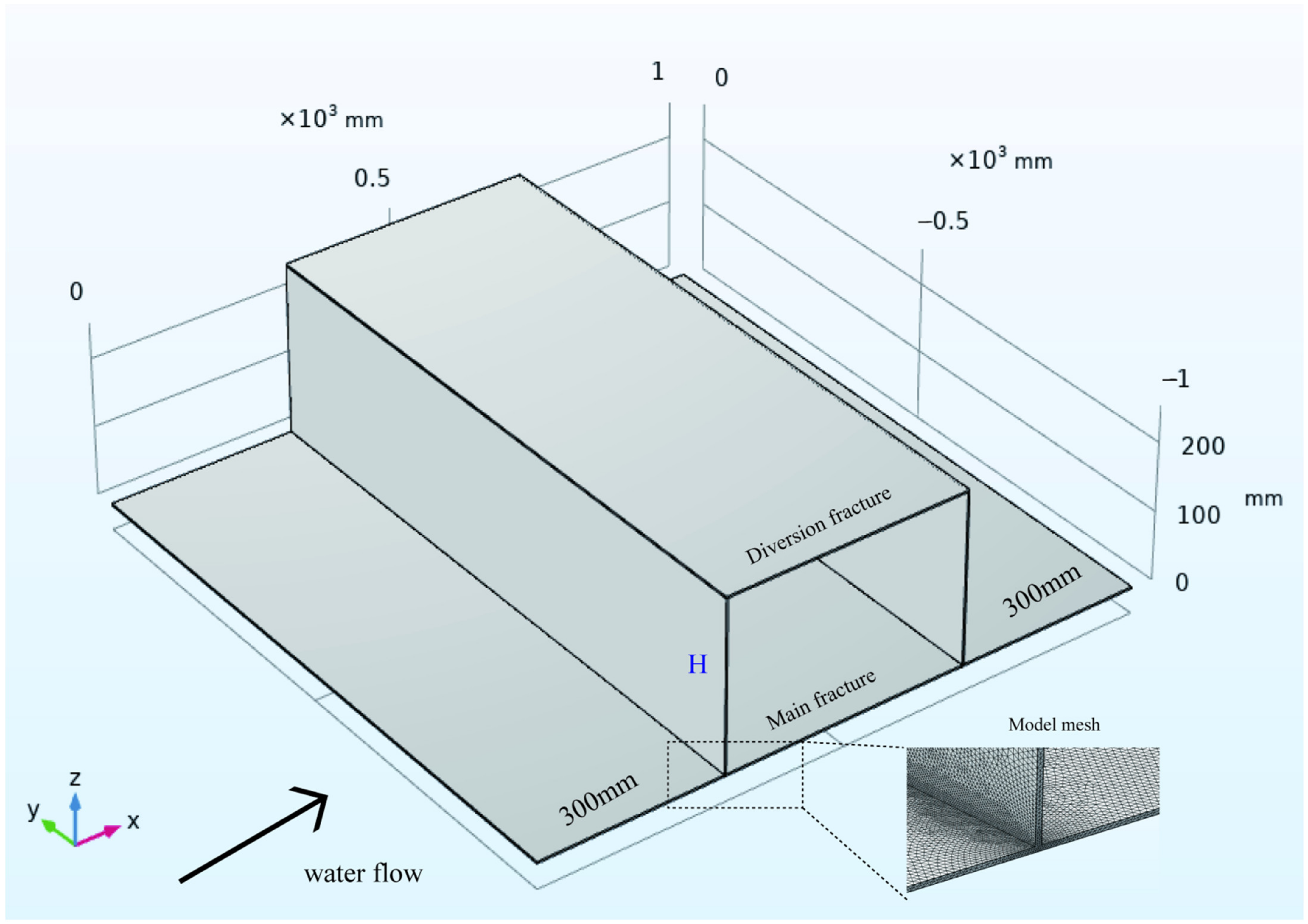
To obtain water flow parameters and solute transport curves for 2D and 3D fractures, the finite-element program COMSOL Multiphysics 6.0 was utilized to resolve the N-S equations. The fracture has dimensions of 1 m in length, 1 m in width, and 3 mm in fracture aperture. A parallel plate model was thus established (Figure 1) to explore the influence of the geometric morphology on solute transport, where H represents the distance between the dual-conduit fractures. Based on this, four 3D DCFs with H values of 100 mm, 150 mm, 200 mm, and 250 mm, respectively, were generated. The intersections of the diversion fracture and main fracture are 300 mm away from the entrance and exit of the main fracture, and the angles between the diversion fracture and main fracture are 90°.
A total of 3.8 million tetrahedral elements were discretized from the constructed fracture system model. The biggest element is 0.1 mm. To accurately reflect the intricate geometry of intersections, a finer element size (around 0.02 mm) was set for the fractures, particularly the intersection part (Figure 1); this indicated that 3.8 million tetrahedral elements were sufficient to obtain a stable and accurate simulation result. In additions, a mesh-size sensitivity analysis approach was used to establish the resolution of the meshes, so as to achieve the mesh independence and numerical stability of the simulation findings, and a high-performance workstation was used for all simulations. It took roughly 2 h to complete each solution for the steady-state flow and took approximately 28 h to complete each solute transport of the mean residence time. It should be noted that the COMSOL Multiphysics package provided a fast equation solver for Equation (1). The results of the solved flow field served as the basis and were coupled with the solute transport model. Meshes were created in this manner by applying slightly different smoothing operations to the original data. This was the least labor-intensive method of constructing the fracture meshes and the convergence of the model could be ensured, while still capturing the small scale of the fracture walls. In addition, because of the proprietary nature of the software, few details about the data smoothing algorithms were available.
Typically, the outflow was configured as a zero-pressure boundary, and the other boundaries were set as nonslip impermeable walls. Water was utilized as the fluid for the fluid properties, featuring a constant density of 1000 kg/m3 and a dynamic viscosity of 0.001 Pa·s. Generally, different Q was applied to the inflow boundary associated with the Reynolds number Re = ρq/(wμ) between 1 and 300, which could be thought of as being within the linear laminar flow regime with minimal turbulent effects. Due to the modest amount of the injected solute and the adoption of the case of diluted solute transport (C0 = 0.1 mol/m3), the initial flow properties would not be affected when the water diffusion coefficient of the solute was set to 1 × 10⁻⁷ m2/s. Considering both advection-dominating and diffusion-dominating transport, the transport behaviors in the 4 fracture cases were evaluated under different flow velocities, and the resulting Peclet number Pe = Q/(wD) ranged from 3 to 30 for the given Q. Injecting a known quantity of tracer at an upstream position and monitoring the variations in the tracer concentration at a downstream location yielded a BTC.
4. Results and Discussion
4.1. Water Flow Test
As can be seen from Table 1, the inlet pressure of fractures shows a clear quadratic relationship with the quantity of flow (R2 > 0.99). Variations in fracture geometry lead to changes in hydraulic parameters. With increases in the value of H, the coefficient A representing the cohesive force increases while the coefficient B representing the inertial force decreases in 2D fractures. The viscosity coefficient increases from 3.75 × 10⁵ to 3.92 × 10⁵, while the inertia coefficient decreases from 7.63 × 10⁷ to 6.94 × 10⁷, and the coefficients A and B are both essentially constant in 3D fractures. The viscosity coefficient ranges from 3.88 × 10⁵ to 3.92 × 10⁵, while the inertia coefficient ranges from 11.6 × 10⁷ to 11.7 × 10⁷. Thus, the Rec varies with geometric parameters in 2D fracture but is not significantly different in 3D. The non-Darcy phenomena are more pronounced the closer the branching in 2D. Moreover, branch fracture geometry controls the flow rate and seepage channel at the intersection.
Although the cohesive forces are not significantly different between 2D and 3D for the same fracture geometry, the inertial forces are significantly different. In comparison with the 2D fracture, the cross-flow of the 3D fractures causes a more pronounced non-Darcy phenomenon. In addition, the Rec of the 2D fracture can be approximately 40% less than that of the 3D fractures, which is attributed to the fact that the increase in the length of the diversion fracture causes the flow to become biased towards the main fracture, which causes the decreased pressure drop loss.
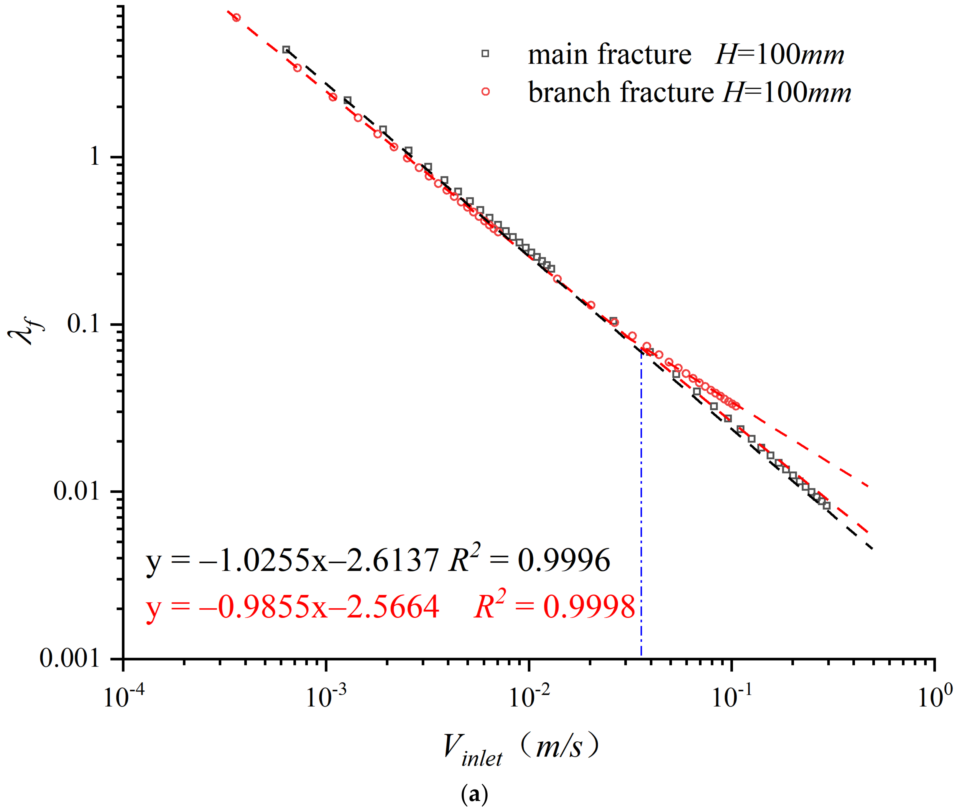
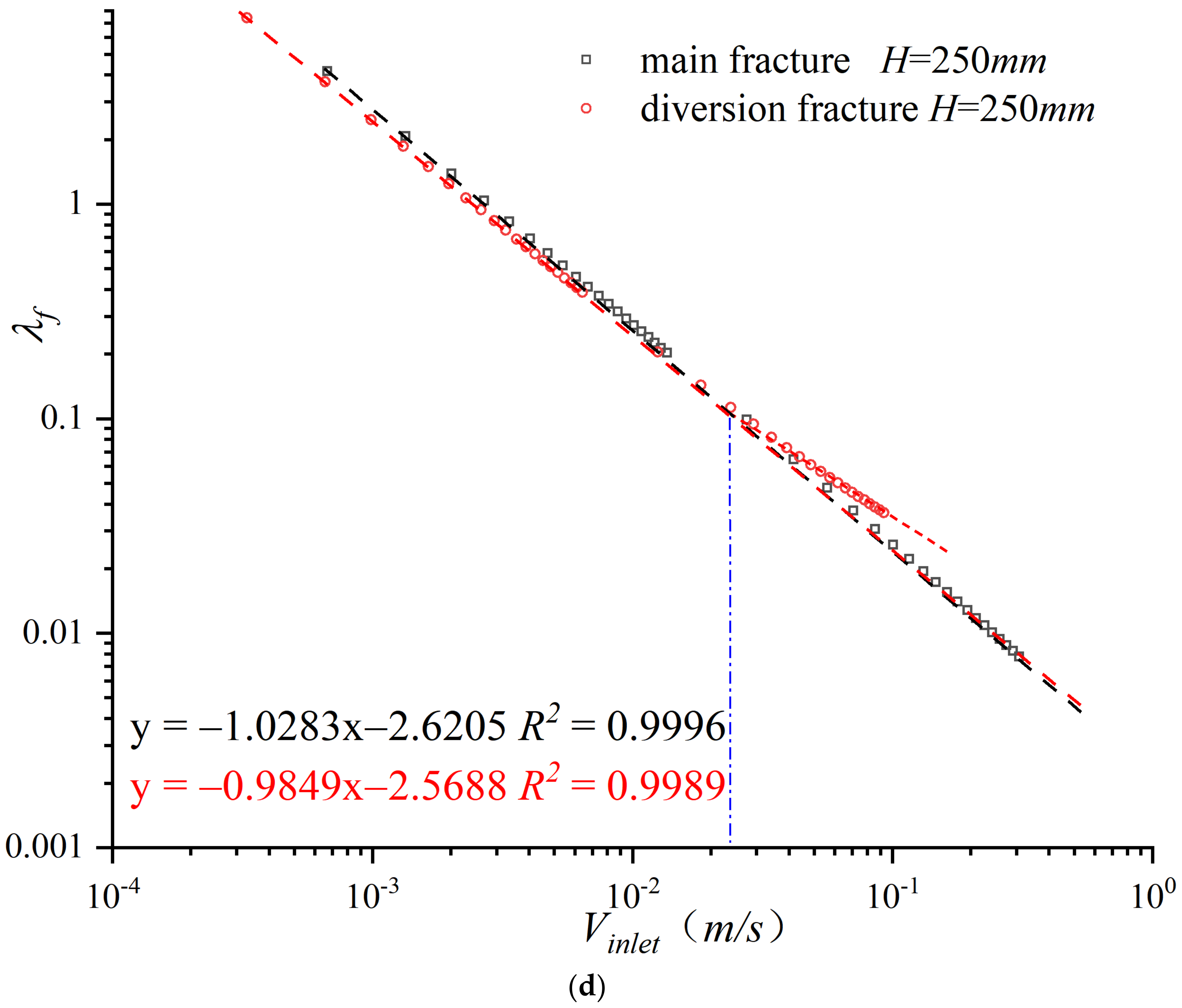
Current research has clearly shown that the coefficient of friction can be related to the flow state characterized by the Reynolds number. The flow curve can then be explicitly and quantitatively divided into two regimes, i.e., the Darcy flow and the Forchheimer flow. As can be seen from Figure 2, when the flow rate is low, the λf and the flow rate show a negative-correlation linear trend in the case of the power exponent. When the flow velocity increases to a certain value (blue dotted line), the downward trend of the friction coefficient of the diversion fracture becomes gentle and the curve presents a nonlinear change. However, the λf of the main fracture is not changed obviously, the main sites responsible for fracture non-Darcy are in the diversion fractures, and the intersection between the main and diversion fracture does not cause significant nonlinearity in the main fracture flow.
4.2. Solute Concentration Distribution
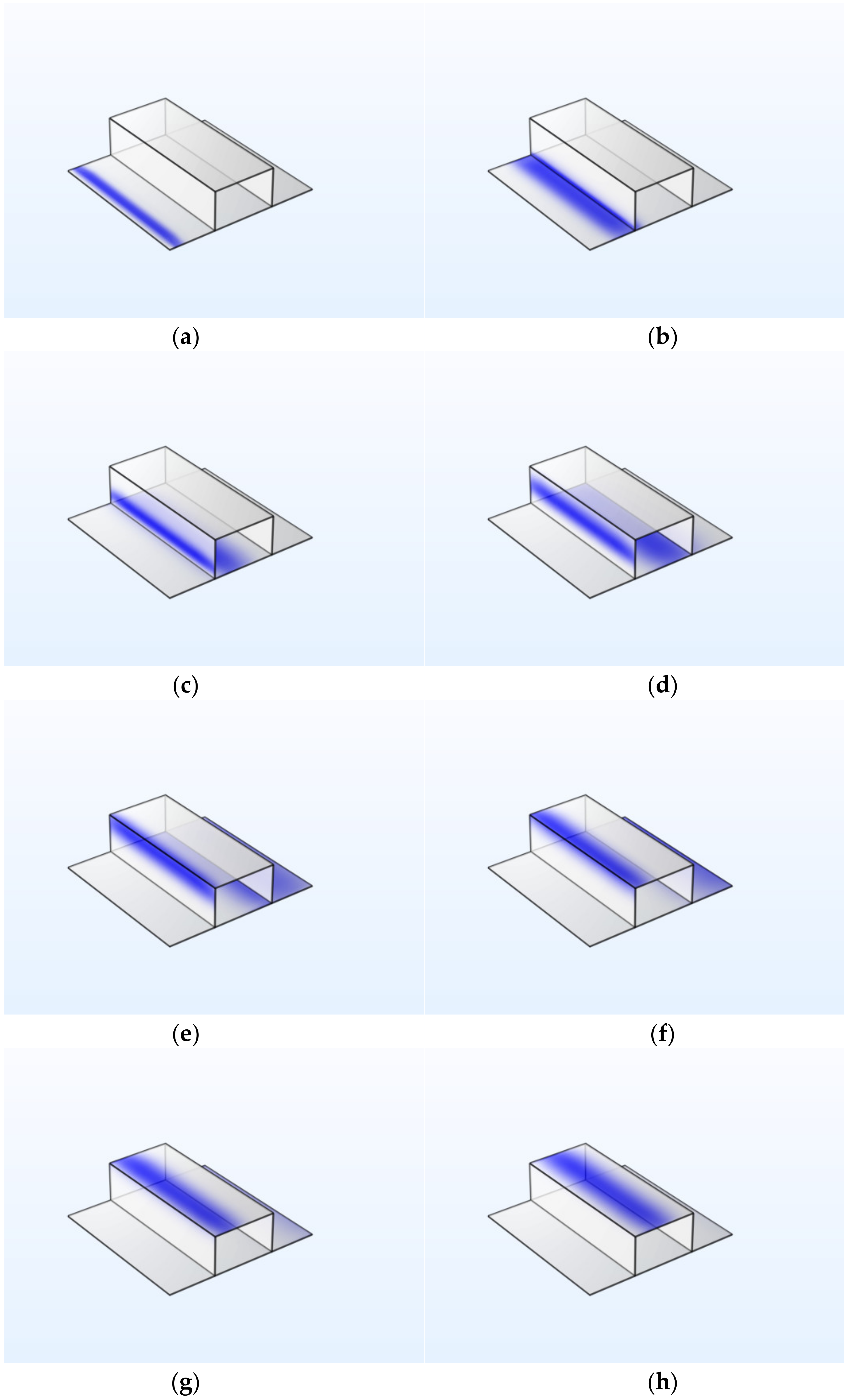
Artificial tracing is extensively used for characterizing rock fracture flow and effective transport parameters [27]. In Figure 3c, after passing the first intersection, the solute transport is observed in the main and diversion fractures, respectively. As shown in Figure 3d–f, due to the different path lengths and flow velocity magnitudes, the first peak is the solute transport curve for the main fracture, while the second peak is the solute transport curve for the diversion fracture, and the concentration field is uniformly distributed along the main flow direction. Over time, the concentration field near the boundary shows only slight variations in concentration along the x-axis. The main reason for this phenomenon is that, under a low Pe number and low flow conditions, the transport process is dominated by diffusion, covering the effect of velocity changes caused by the fracture boundary layer. In the case of diversion fractures, the low-flow velocity zone formed at the corner of the diversion fractures is clearly demonstrated as the main cause of non-Darcy flow. As a result, due to the influence of the low-flow velocity zone at the corner, the concentration field appears inhomogeneous while approaching the boundary layer.
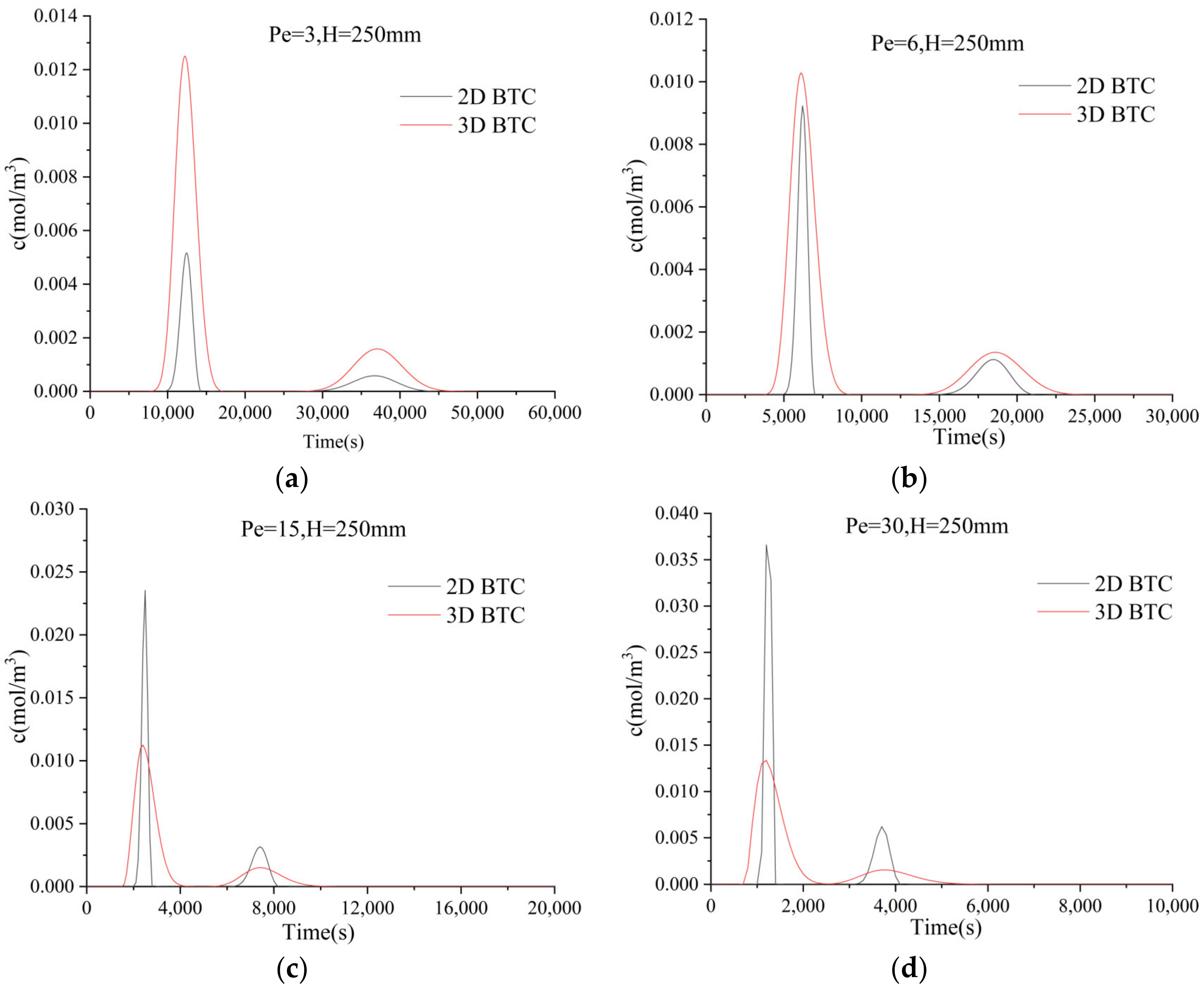
Figure 4 shows the experimental BTCs for the different flow rates and H values, where Figure 4a–d represent H = 250 mm, and the black and red curves represent 2D and 3D, respectively. The BTCs in each graph present a double-peak phenomenon, showing significant differences in propagation times in the main and diversion fractures.
As shown in Figure 4, the measured BTCs are fitted with the WSADE, and the associated transport properties are listed in Table 2 and Table 3, where it can be observed that the WSADE solution matches well with the measured BTCs. When the flow rate is low (Pe = 3), the solute flows slower in the diversion fracture, its value of dispersion is higher relative to the main fracture (D1 and D2 in Table 3), and the diffusion is more evident in the path of the diversion fracture (Figure 4a). As the Pe increases, the BTC curves of the fractures become steeper (Figure 4b–d) and the role of convection in solute transport increases while the dispersion decreases. Compared to the 2D fracture, the dispersion coefficient of the 3D fractures increases when the Pe > 6 (Figure 4b–d). Notably, as depicted from the concentration distributions in Figure 4a–d, the distance between the two peaks decreases with an increasing Pe number, thereby resulting in a relatively late arrival of the peak in the diversion fracture. On the other side, the diffusion coefficient of the solute increases with increases in the flow velocity (Table 3).
The distance between the main fracture and the diversion fracture (H) has a significant effect on the flow distribution and thus on the solute transfer of the solutes in the fissure. As can be seen from Table 3, the length of the diversion fracture increases, the flow velocity of the diversion fracture decreases, and the flow velocity of the main fracture increases. As a result, the diffusion coefficient of the diversion fracture (D2) increases and the diffusion coefficient of the main fracture (D1) decreases. The above deductions are summarized, since BTCs can bring information on underground geometry.
When Pe = 30, the DCF is in the linear region, and the water flow ratio between the main fracture and the diversion fracture (Q1/Q2) is the same. Theoretically, when the fracture solute transport is in the streamlined routing model, the distribution of the flow rates leads to the distribution of outlet concentrations. The ratio of w1/w2, which represents the concentration ratio between the main fracture and diversion fracture, should be the same as the fracture flow ratio. In addition, by comparing Table 1 and Table 3, it can be found that the ratio of water flow is greater than the concentration between the ratio of w1/w2, indicating the essential role of the streamline routing mode in the solute transfer. With increasing flow rates, the ratio of w1/w2 tends to be closer to the flow ratio; due to this, the effect of the complete mixing mode is weakened in the solute transfer process. In particular, the ratios of w1/w2 are significantly larger in 3D than those in 2D, indicating that the streamlined routing mode is more important in the 3D fracture.
4.3. Discussion
Herein, the advective component of solute transport was explored through intersecting rough-walled fractures. Fundamentally, the multidirectional boundary layer causes the mixing trends and deviations from the 3D parallel plate models that are observed. Some research [28,29] has shown that the interaction forces of liquids on domain boundaries are the main cause of viscous forces. The locations of the main conduit and the diversion conduit affect the migration of the flow and solutes. The further apart the fractures are from each other, the greater the variation in the dispersion coefficients of their two peaks. If the two peaks are completely separated from each other, the lengths of the two conduits may be significantly different. Therefore, a large length contrast between the two conduits can be obtained when the two peaks are completely separated. In a previous experimental study [15], the dual-conduit constructions were more prone to exhibit dual-peaked BTCs as the flow rate rose; the results provide detailed information that should help researchers better understand the transport processes in these structures.
The boundary layer of the fracture is one of the main causes of the non-Darcy effect of water flow, which affects the migration of solutes at the intersection when the flow is in the Darcy zone. As shown in Table 2, the ratio of w1/w2 becomes larger as the flow rate increases with increasing H values under the same hydraulic and geometry conditions, and the ratio of w1/w2 is larger for 3D than that for 2D. It was conventionally considered that the solute distribution in the fracture at the intersection is linearly related to the flow. However, as shown in Table 1 and Table 2, the boundary layer affects the diffusion of solute transport at the same flow velocity.
The boundary layer, i.e., a fluid layer that is stagnant in rock fracture media, is reported to exist. During the study of solute transport, although the water flow is in a linear state and vortices are not clearly observed, the solute transport transfer in the fissure is influenced by the Pe number due to the change in the boundary layer thickness, which forms a hysteresis region within the boundary layer, thereby resulting in different BTC characteristics. In addition, the multidimensional nature of the 3D DCF makes its boundary layer range relatively larger and endows it with a more pronounced effect on solute transport. Secchi et al. [30] demonstrated that a fluid ceiling attached to a solid wall has solid-like qualities. In a rather small area, the density and viscosity also rise dramatically. Wu et al. [31] proved that the existence of a thin, nonflowing layer in microchannels is the outcome of fluid–solid interaction through experimental research. There is less flow space due to the existence of the boundary layer, which also increases flow resistance. Considerable attempts have been made by academics to describe the thickness of the boundary layer. When a fluid–solid interaction creates the boundary layer, its thickness depends on the characteristics of both the fluid and the solid wall [32]. The geometry of the fracture changes the distribution of the boundary layer, which affects the water flow and solute transfer. However, the 3D fracture has a greater interference effect than the 2D fracture because of its multidimensional boundary layer.
5. Conclusions
The water flow and solute transport process in dual-conduit structures were herein studied numerically and investigated. The Navier–Stokes and advection–diffusion equations were numerically solved to simulate the conservative water flow and solute transport. Some general conclusions from this study are summarized as follows:
- Based on the numerical results, the Forchheimer equations can more accurately describe the nonlinear fracture flow characteristics in DCFs. The further apart the branch fractures are from each other, the more the coefficient A representing the cohesive force increases while the coefficient B representing the inertial force decreases in 2D fractures, and the coefficients A and B are essentially constant in 3D fractures.
- Relative to the 2D fracture, the 3D DCFs cause a more pronounced non-Darcy phenomenon. Additionally, the Rec of 2D fractures can be approximately 40% less than that of 3D fractures. With an increasing flow rate, the friction coefficient in the bypass is nonlinearly related to the flow rate at exponential conditions, demonstrating the diversion fractures as the main scene of the non-Darcy phenomenon.
- The BTC in each graph shows a double-peak phenomenon with significant differences in propagation times in the main and diversion fractures due to the variation in flow rates. Dual-peaked BTCs can be reproduced by the WSADE model. Furthermore, the further apart the branch fractures are from each other, the larger the Pe number, when the values of parameter D1 of WSADE decrease and parameter D2 and the ratio of w1/w2 increase. Moreover, in the same geometry and flow conditions, the BTC of the 2D fracture is steeper than that of the 3D fracture, and this phenomenon becomes more obvious with increases in Pe.
- Both the complete mixing model and the streamlined routing model affect the transport of fractured solutes, and the streamlined routing mode plays a major role in the solute transfer. With increasing flow rates, the effect of the complete mixing mode is weakened in the solute transport. From a statistics point of view, the streamlined routing mode is more obvious in 3D than that in 2D.
In summary, DCFs caused by distance can influence the nonlinear flow behavior and the outlet solute rate distribution. The current study is a complementary work to a previous study, revealing the effects of the spatial distribution and flow rate. Overall, this work provides a method to estimate the fracture structure by the parametric evaluation of the Forchheimer equation and WSADE coefficients.
Author Contributions
Conceptualization, Y.L.; Data curation, Y.L.; Formal analysis, Y.L.; Funding acquisition, Y.L.; Investigation, Y.L.; Methodology, Y.L.; Project administration, Y.L.; Resources, Y.L.; Supervision, L.C.; Validation, Y.L., L.C. and Y.S.; Visualization, Y.L.; Writing—Original draft, Y.L.; Writing—Review and editing, L.C. and Y.S. All authors have read and agreed to the published version of the manuscript.
Funding
This research received no external funding.
Data Availability Statement
Not applicable.
Acknowledgments
We would like to express our sincerest gratitude for the support from Comsol Simulation.
Conflicts of Interest
The authors declare no conflict of interest.
References
- Chen, Y.; Ma, G.; Wang, H. Heat Extraction Mechanism in a Geothermal Reservoir with Rough-Walled Fracture Networks. Int. J. Heat Mass Transf. 2018, 126, 1083–1093. [Google Scholar] [CrossRef]
- Chen, Y.; Ma, G.; Wang, H. The Simulation of Thermo-Hydro-Chemical Coupled Heat Extraction Process in Fractured Geothermal Reservoir. Appl. Therm. Eng. 2018, 143, 859–870. [Google Scholar] [CrossRef]
- Ma, G.; Chen, Y.; Jin, Y.; Wang, H. Modelling Temperature-Influenced Acidizing Process in Fractured Carbonate Rocks. Int. J. Rock Mech. Min. 2018, 105, 73–84. [Google Scholar] [CrossRef]
- Fan, L.F.; Wu, Z.J.; Wan, Z.; Gao, J.W. Experimental Investigation of Thermal Effects on Dynamic Behavior of Granite. Appl. Therm. Eng. 2017, 125, 94–103. [Google Scholar] [CrossRef]
- Dai, F.; Wei, M.D.; Xu, N.W.; Ma, Y.; Yang, D.S. Numerical Assessment of the Progressive Rock Fracture Mechanism of Cracked Chevron Notched Brazilian Disc Specimens. Rock Mech. Rock Eng. 2014, 48, 463–479. [Google Scholar] [CrossRef]
- Johnson, J.; Brown, S.; Stockman, H. Fluid Flow and Mixing in Rough-Walled Fracture Intersections. J. Geophys. Res.-Sol. Earth 2006, 111, 2169–9313. [Google Scholar] [CrossRef]
- Tsang, C.-F.; Neretnieks, I.; Tsang, Y. Hydrologic Issues Associated with Nuclear Waste Repositories. Water Resour. Res. 2015, 51, 6923–6972. [Google Scholar] [CrossRef]
- Sayed, M.; Chang, F.; Cairns, A.J. Low-Viscosity Single Phase Acid System for Acid Fracturing in Deep Carbonate Reservoirs. MRS Commun. 2021, 11, 796–803. [Google Scholar] [CrossRef]
- Ranjith, P.G.; Darlington, W. Nonlinear Single-Phase Flow in Real Rock Joints. Water Resour. Res. 2007, 43, W09502. [Google Scholar] [CrossRef]
- Huang, H.; Babadagli, T.; Li, H.A.; Develi, K.; Wei, G. Effect of Injection Parameters on Proppant Transport in Rough Vertical Fractures: An Experimental Analysis on Visual Models. J. Pet. Sci. Eng. 2019, 180, 380–395. [Google Scholar] [CrossRef]
- Zhong, Z.; Ding, J.; Hu, Y. Size Effect on the Hydraulic Behavior of Fluid Flow through Rough-Walled Fractures: A Case of Radial Flow. Hydrogeol. J. 2021, 30, 97–109. [Google Scholar] [CrossRef]
- Luo, S.; Zhao, Z.; Peng, H.; Pu, H. The Role of Fracture Surface Roughness in Macroscopic Fluid Flow and Heat Transfer in Fractured Rocks. Int. J. Rock. Mech. Min. Sci. 2016, 87, 29–38. [Google Scholar] [CrossRef]
- Fan, L.F.; Wang, H.D.; Wu, Z.J.; Zhao, S.H. Effects of Angle Patterns at Fracture Intersections on Fluid Flow Nonlinearity and Outlet Flow Rate Distribution at High Reynolds Numbers. Int. J. Rock. Mech. Min. Sci. 2019, 124, 104136. [Google Scholar] [CrossRef]
- Zou, L.; Jing, L.; Cvetkovic, V. Modeling of Flow and Mixing in 3D Rough-Walled Rock Fracture Intersections. Adv. Water Resour. 2017, 107, 1–9. [Google Scholar] [CrossRef]
- Wang, C.; Majdalani, S.; Guinot, V.; Jourde, H. Solute Transport in Dual Conduit Structure: Effects of Aperture and Flow Rate. J. Hydrol. 2022, 613, 128315. [Google Scholar] [CrossRef]
- Wang, C.; Wang, X.; Majdalani, S.; Guinot, V.; Jourde, H. Influence of Dual Conduit Structure on Solute Transport in Karst Tracer Tests: An Experimental Laboratory Study. J. Hydrol. 2020, 590, 125255. [Google Scholar] [CrossRef]
- Chen, L.; Huang, Y. Experimental Study and Characteristic Finite Element Simulation of Solute Transport in a Cross-Fracture. Geosci. Front. 2016, 7, 963–967. [Google Scholar] [CrossRef]
- Berkowitz, B. Characterizing Flow and Transport in Fractured Geological Media: A Review. Adv. Water Resour. 2002, 25, 861–884. [Google Scholar] [CrossRef]
- Xing, K.; Qian, J.; Zhao, W.; Ma, H.; Ma, L. Experimental and Numerical Study for the Inertial Dependence of Non-Darcy Coefficient in Rough Single Fractures. J. Hydrol. 2021, 603, 127148. [Google Scholar] [CrossRef]
- Liu, X.; Chen, D.; Li, M.; Li, Y.; Yang, X. Characteristics of Fluid Flow and Solute Transport in Multicrossed Rough Rock Fractures Based on Three-Dimensional Simulation. IOP Conf. Ser. Earth Environ. Sci. 2021, 861, 072095. [Google Scholar] [CrossRef]
- Pot, V.; Genty, A. Dispersion Dependence on Retardation in a Real Fracture Geometry Using Lattice-Gas Cellular Automaton. Adv. Water Resour. 2007, 30, 273–283. [Google Scholar] [CrossRef]
- Benson, D.A.; Meerschaert, M.M. A Simple and Efficient Random Walk Solution of Multi-Rate Mobile/Immobile Mass Transport Equations. Adv. Water Resour. 2009, 32, 532–539. [Google Scholar] [CrossRef]
- Berkowitz, B.; Scher, H. Exploring the Nature of Non-Fickian Transport in Laboratory Experiments. Adv. Water Resour. 2009, 32, 750–755. [Google Scholar] [CrossRef]
- Majdalani, S.; Guinot, V.; Delenne, C.; Gebran, H. Modelling Solute Dispersion in Periodic Heterogeneous Porous Media: Model Benchmarking against Intermediate Scale Experiments. J. Hydrol. 2018, 561, 427–443. [Google Scholar] [CrossRef]
- Zhao, X.; Chang, Y.; Wu, J.; Peng, F. Laboratory Investigation and Simulation of Breakthrough Curves in Karst Conduits with Pools. Hydrogeol. J. 2017, 25, 2235–2250. [Google Scholar] [CrossRef]
- Field, M.S.; Leij, F.J. Solute Transport in Solution Conduits Exhibiting Multi-Peaked Breakthrough Curves. J. Hydrol. 2012, 440–441, 26–35. [Google Scholar] [CrossRef]
- Goldscheider, N.; Meiman, J.; Pronk, M.; Smart, C. Tracer Tests in Karst Hydrogeology and Speleology. Int. J. Speleol. 2008, 37, 27–40. [Google Scholar] [CrossRef]
- Sedahmed, M.; Coelho, V.; Warda, H.A. An Improved Multicomponent Pseudopotential Lattice Boltzmann Method for Immiscible Fluid Displacement in Porous Media. Phys. Fluids 2022, 34, 023102. [Google Scholar] [CrossRef]
- Sedahmed, M.; Rodrigo, C.V.; Nuno, A.M.; Wahba, E.M.; Warda, H.A. Study of Fluid Displacement in Three-Dimensional Porous Media with an Improved Multicomponent Pseudopotential Lattice Boltzmann Method. Phys. Fluids 2022, 34, 103303. [Google Scholar] [CrossRef]
- Secchi, E.; Marbach, S.; Niguès, A.; Stein, D.; Siria, A.; Bocquet, L. Massive Radius-Dependent Flow Slippage in Carbon Nanotubes. Nature 2016, 537, 210–213. [Google Scholar] [CrossRef]
- Wu, K.; Chen, Z.; Li, J.; Li, X.; Xu, J.; Dong, X. Wettability Effect on Nanoconfined Water Flow. Proc. Natl. Acad. Sci. USA 2017, 114, 3358–3363. [Google Scholar] [CrossRef] [PubMed]
- Huang, Y.; Yang, Z.; He, Y.; Wang, X. An Overview on Nonlinear Porous Flow in Low Permeability Porous Media. Theor. Appl. Mech. Lett. 2013, 3, 022001. [Google Scholar] [CrossRef]
Figure 1.
Schematic diagram of the 3D fracture model for the fluid flow test.

Figure 2.
Variations of the friction factor with flow rates in different H values: (a) 100 mm; (b) 150 mm; (c) 200 mm; and (d) 250 mm.
Figure 2.
Variations of the friction factor with flow rates in different H values: (a) 100 mm; (b) 150 mm; (c) 200 mm; and (d) 250 mm.


Figure 3.
Solute concentration distributions at different times when Pe = 15 and H = 250 mm. (a–h) is when time = 200 s, 700 s, 1200 s, 1700 s, 2200 s, 2700 s, 3200 s and 3700 s, respectively.
Figure 3.
Solute concentration distributions at different times when Pe = 15 and H = 250 mm. (a–h) is when time = 200 s, 700 s, 1200 s, 1700 s, 2200 s, 2700 s, 3200 s and 3700 s, respectively.

Figure 4.
The BTCs of the 2D and 3D fractures: (a) Pe = 3; (b) Pe = 6; (c) Pe = 15; (d) Pe = 30.


Table 1.
Curve-fitting parameters of the Forchheimer’s law in 2D and 3D fractures.
| Fracture | H (mm) | A (105) | B (107) | Rec | R2 | Q1/Q2 |
|---|---|---|---|---|---|---|
| 2D | 100 | 3.75 | 7.63 | 54.61 | 0.998 | 1.60 |
| 150 | 3.82 | 7.88 | 53.86 | 0.997 | 1.88 | |
| 200 | 3.88 | 7.25 | 59.46 | 0.996 | 2.14 | |
| 250 | 3.93 | 6.94 | 62.92 | 0.999 | 2.41 | |
| 3D | 100 | 3.92 | 11.6 | 37.55 | 0.999 | 1.63 |
| 150 | 3.88 | 11.7 | 36.85 | 0.999 | 1.89 | |
| 200 | 3.88 | 11.7 | 36.85 | 0.998 | 2.17 | |
| 250 | 3.92 | 11.6 | 37.55 | 0.999 | 2.43 |
Table 2.
Curve-fitting parameters of the WSADE in the 2D fracture.
| Pe | H (mm) | v1 (m/s) | v2 (m/s) | D1 (m2/s) | D2 (m2/s) | w1/w2 |
|---|---|---|---|---|---|---|
| 3 | 250 | 8.06 × 10⁻⁵ | 2.72 × 10⁻⁵ | 0.0121 | 0.0688 | 2.39 |
| 200 | 7.79 × 10⁻⁵ | 3.21 × 10⁻⁵ | 0.0132 | 0.0656 | 2.06 | |
| 150 | 7.65 × 10⁻⁵ | 3.82 × 10⁻⁵ | 0.0197 | 0.0621 | 1.79 | |
| 100 | 7.53 × 10⁻⁵ | 4.61 × 10⁻⁵ | 0.0191 | 0.0598 | 1.52 | |
| 6 | 250 | 1.67 × 10⁻⁴ | 5.45 × 10⁻⁵ | 0.0083 | 0.13 | 2.44 |
| 200 | 1.59 × 10⁻⁴ | 6.37 × 10⁻⁵ | 0.0096 | 0.138 | 2.12 | |
| 150 | 1.48 × 10⁻⁴ | 7.58 × 10⁻⁵ | 0.0111 | 0.149 | 1.84 | |
| 100 | 1.40 × 10⁻⁴ | 9.98 × 10⁻⁵ | 0.0122 | 0.162 | 1.55 | |
| 15 | 250 | 4.21 × 10⁻⁴ | 1.35 × 10⁻⁴ | 0.0065 | 0.233 | 2.73 |
| 200 | 4.02 × 10⁻⁴ | 1.58 × 10⁻⁴ | 0.0074 | 0.174 | 2.22 | |
| 150 | 3.88 × 10⁻⁴ | 1.89 × 10⁻⁴ | 0.0083 | 0.141 | 1.9 | |
| 100 | 3.76 × 10⁻⁴ | 2.27 × 10⁻⁴ | 0.0102 | 0.143 | 1.53 | |
| 30 | 250 | 7.75 × 10⁻⁴ | 2.70 × 10⁻⁴ | 0.0041 | 0.272 | 2.84 |
| 200 | 7.65 × 10⁻⁴ | 3.13 × 10⁻⁴ | 0.0083 | 0.162 | 2.30 | |
| 150 | 7.59 × 10⁻⁴ | 3.7 × 10⁻⁴ | 0.0076 | 0.129 | 1.93 | |
| 100 | 7.51 × 10⁻⁴ | 4.55 × 10⁻⁴ | 0.012 | 0.097 | 1.52 |
Table 3.
3D burst WSADE curve fit parameters.
| Pe | H (mm) | v1 (m/s) | v2 (m/s) | D1 (m2/s) | D2 (m2/s) | w1/w2 |
|---|---|---|---|---|---|---|
| 3 | 250 | 7.75 × 10⁻⁵ | 2.7 × 10⁻⁵ | 0.142 | 0.113 | 3.50 |
| 200 | 7.65 × 10⁻⁵ | 3.16 × 10⁻⁵ | 0.144 | 0.107 | 3.22 | |
| 150 | 7.59 × 10⁻⁵ | 3.75 × 10⁻⁵ | 0.149 | 0.113 | 2.92 | |
| 100 | 7.51 × 10⁻⁵ | 4.05 × 10⁻⁵ | 0.156 | 0.111 | 2.67 | |
| 6 | 250 | 1.64 × 10⁻⁴ | 5.37 × 10⁻⁵ | 0.117 | 0.132 | 3.57 |
| 200 | 1.61 × 10⁻⁴ | 6.32 × 10⁻⁵ | 0.118 | 0.134 | 3.35 | |
| 150 | 1.53 × 10⁻⁴ | 7.47 × 10⁻⁵ | 0.124 | 0.138 | 3.08 | |
| 100 | 1.45 × 10⁻⁴ | 9.02 × 10⁻⁵ | 0.135 | 0.162 | 2.82 | |
| 15 | 250 | 4.28 × 10⁻⁴ | 1.35 × 10⁻⁴ | 0.097 | 0.164 | 3.93 |
| 200 | 4.16 × 10⁻⁴ | 1.56 × 10⁻⁴ | 0.153 | 0.152 | 3.64 | |
| 150 | 4.01 × 10⁻⁴ | 1.85 × 10⁻⁴ | 0.178 | 0.164 | 3.39 | |
| 100 | 3.89 × 10⁻⁴ | 2.39 × 10⁻⁴ | 0.213 | 0.143 | 3.06 | |
| 30 | 250 | 8.78 × 10⁻⁴ | 2.7 × 10⁻⁴ | 0.0334 | 0.224 | 4.59 |
| 200 | 8.69 × 10⁻⁴ | 3.13 × 10⁻⁴ | 0.0184 | 0.232 | 4.14 | |
| 150 | 8.62 × 10⁻⁴ | 3.7 × 10⁻⁴ | 0.0100 | 0.221 | 3.69 | |
| 100 | 8.54 × 10⁻⁴ | 4.54 × 10⁻⁴ | 0.0056 | 0.191 | 3.15 |
Disclaimer/Publisher’s Note: The statements, opinions and data contained in all publications are solely those of the individual author(s) and contributor(s) and not of MDPI and/or the editor(s). MDPI and/or the editor(s) disclaim responsibility for any injury to people or property resulting from any ideas, methods, instructions or products referred to in the content. |
© 2023 by the authors. Licensee MDPI, Basel, Switzerland. This article is an open access article distributed under the terms and conditions of the Creative Commons Attribution (CC BY) license (https://creativecommons.org/licenses/by/4.0/).
Share and Cite
MDPI and ACS Style
Li, Y.; Chen, L.; Shi, Y. Influence of 3D Fracture Geometry on Water Flow and Solute Transport in Dual-Conduit Fracture. Water 2023, 15, 1754. https://doi.org/10.3390/w15091754
AMA Style
Li Y, Chen L, Shi Y. Influence of 3D Fracture Geometry on Water Flow and Solute Transport in Dual-Conduit Fracture. Water. 2023; 15(9):1754. https://doi.org/10.3390/w15091754
Chicago/Turabian StyleLi, Yubo, Linjie Chen, and Yonghong Shi. 2023. "Influence of 3D Fracture Geometry on Water Flow and Solute Transport in Dual-Conduit Fracture" Water 15, no. 9: 1754. https://doi.org/10.3390/w15091754
Note that from the first issue of 2016, this journal uses article numbers instead of page numbers. See further details here.