Evaluation of Statistical PMP Considering RCP Climate Change Scenarios in Republic of Korea

Abstract

Extreme rainfall and floods have increased in frequency and severity in recent years, due to climate change and urbanization. Consequently, interest in estimating the probable maximum precipitation (PMP) has been burgeoning. The World Meteorological Organization (WMO) recommends two types of methods for calculating the PMP: hydrometeorological and statistical methods. This study proposes a modified Hershfield’s nomograph method and assesses the changes in PMP values based on the two representative concentration pathway (RCP4.5 and RCP8.5) scenarios in South Korea. To achieve the intended objective, five techniques were employed to compute statistical PMPs (SPMPs). Moreover, the most suitable statistical method was selected by comparing the calculated SPMP with the hydrometeorological PMP (HPMP), by applying statistical criteria. Accordingly, SPMPs from the five methods were compared with the HPMPs for the historical period of 2020 and the future period of 2100 for RCP 4.5 and 8.5 scenarios, respectively. The results confirmed that the SPMPs from the modified Hershfield’s nomograph showed the smallest MAE (mean absolute error), MAPE (mean absolute percentage error), and RMSE (root mean square error), which are the best results compared with the HPMP with an average SPMP/HPMP ratio of 0.988 for the 2020 historical period. In addition, Hershfield’s method with varying $K_M$ exhibits the worst results for both RCP scenarios, with SPMP/HPMP ratios of 0.377 for RCP4.5 and 0.304 for RCP8.5, respectively. On the contrary, the modified Hershfield’s nomograph was the most appropriate method for estimating the future SPMPs: the average ratios were 0.878 and 0.726 for the 2100 future period under the RCP 4.5 and 8.5 scenarios, respectively, in South Korea.

1. Introduction

The World Meteorological Organization [1,2] defines the probable maximum precipitation (PMP) as the maximum depth of precipitation for a given rainfall duration and area. PMP is used to estimate the probable maximum flood (PMF), which is generally utilized to design large hydraulic structures. The PMP is utilized worldwide for dam safety assessments. In many countries, dam managers are legally required to use PMPs [3]. Changes in the magnitude and pattern of extreme rainfall events require periodic updates for planning the repair work [4], and PMP is important for designing high-risk hydraulic structures [5].

Recently, abnormal climate phenomena have been reported worldwide, and extreme rainfall due to climate change and urbanization has become increasingly common. The South Korean Ministry of Works [6] calculated the hydrometeorological PMP in 1988 using meteorological data up to 1987, and published a PMP map. In addition, the Ministry of Land, Infrastructure and Transport (MLIT) updated the map of PMP in 2000 [7] based on the WMO report [1,2]. However, the PMP was recalculated in 2004 because the observed rainfall during typhoon “Rusa” in 2002 exceeded the PMP from a specific area [8]. Additionally, after establishing the calculation procedure guidelines for the PMP and PMF in 2008 [9], the PMP was estimated based on the hydrometeorological method conducted in 2020 in Korea [10]. The PMP is based on previously recorded extreme rainfall and, should be periodically updated to include new extreme rainfall [5]. Moreover, the PMP is very spatially volatile, due to the geographical complexity in South Korea. Therefore, it is crucial for actual climate change adaptation planning to determine how future PMPs will change in the regions of interest [11,12]. Furthermore, the uncertainties associated with PMP estimation should be considered when calculating the PMP [13,14].

The most widely used methods for estimating PMP are hydrometeorological and statistical methods. The former considers the maximal ratio between the maximum precipitation during a specific period of the year and the actual precipitation during heavy rain [2,12]. The statistical method developed by Hershfield [15] focuses on frequency analysis and the effect of outliers on the mean and standard deviation of annual maximum precipitation at locations of interest [2,15]. To overcome data unavailability, a reasonable range of PMP values can be calculated using statistical methods [13].

Hershfield initially analyzed the maximum annual precipitation for a total of 95,000 station-years corresponding to 2645 stations. Statistical methods are limited when historical rainfall data are insufficient [16]. Hershfield originally suggested a value of 15 for the frequency factor ($K_M=15)$. However, the frequency factor $K_M=15$ was too high for wet areas [17] and was relatively large for the return period of PMP in Korea, compared to those in the literature [18]. The minimum period required for calculating the statistical PMP in Korea was selected as 43 years, and it was recommended to augment it by 10% for an observation period of less than 30 years [19]. Koutsoyiannis estimated the PMP using Hershfield’s rainfall data based on the generalized extreme value (GEV) distribution and using a shape parameter as a linear function of the mean annual maximum precipitation, and then concluded that the PMP return period corresponded to 60,000 years [20]. Generally, Hershfield’s method has been utilized in many countries globally because it only requires the annual maximum daily precipitation [21,22].

Other methods, such as a probabilistic approach, have been studied for decades to estimate the PMP, but limitations persist, despite the progress in their development. Additional research is needed to effectively apply it while considering the impact of climate change [23]. PMP calculations through the application of climate change scenarios can predict future PMP values from abnormalities in the data [16]. The PMP increases under climate change, which must be considered to design and maintain the hydro-infrastructure in the water engineering field [24]. Rousseau et al. [25] developed the methodology based on the non-stationary frequency analysis to evaluate PMP under changing climate conditions. Rastogi et al. [26] revealed increasing trends in the future PMP using Weather Research and Forecasting (WRF) simulations. Moreover, atmospheric warming is an important factor that can increase the PMP. Therefore, the future PMP and the magnitude of the increase should be estimated to address the global risk of flood damage due to the substantial increase in water vapor concentrations [27].

This study primarily aims to determine an appropriate statistical method for estimating PMP for the 2020 historical period and future 2100 period, using five statistical methods: (1) Hershfield’s fixed frequency factor $K_M=15$ [15], (2) Hershfield’s method with varying $K_M$ at each site, (3) Hershfield’s original nomograph [28], (4) modified Hershfield’s nomograph, and (5) Chow’s frequency factor method (T = 60,000) [29]. Therefore, the estimated statistical PMP (SPMP) was compared with the hydrometeorological PMP (HPMP) for both 2020 and 2100. Finally, the estimated SPMPs from the five methods were compared with the HPMP for 2020, based on SPMP/HPMP ratio and several statistical measures. Moreover, the estimated SPMPs were compared with the HPMPs for the future period of 2100, calculated from the RCP 4.5 and 8.5 scenarios.

2. Study Area and Datasets

2.1. Study Area

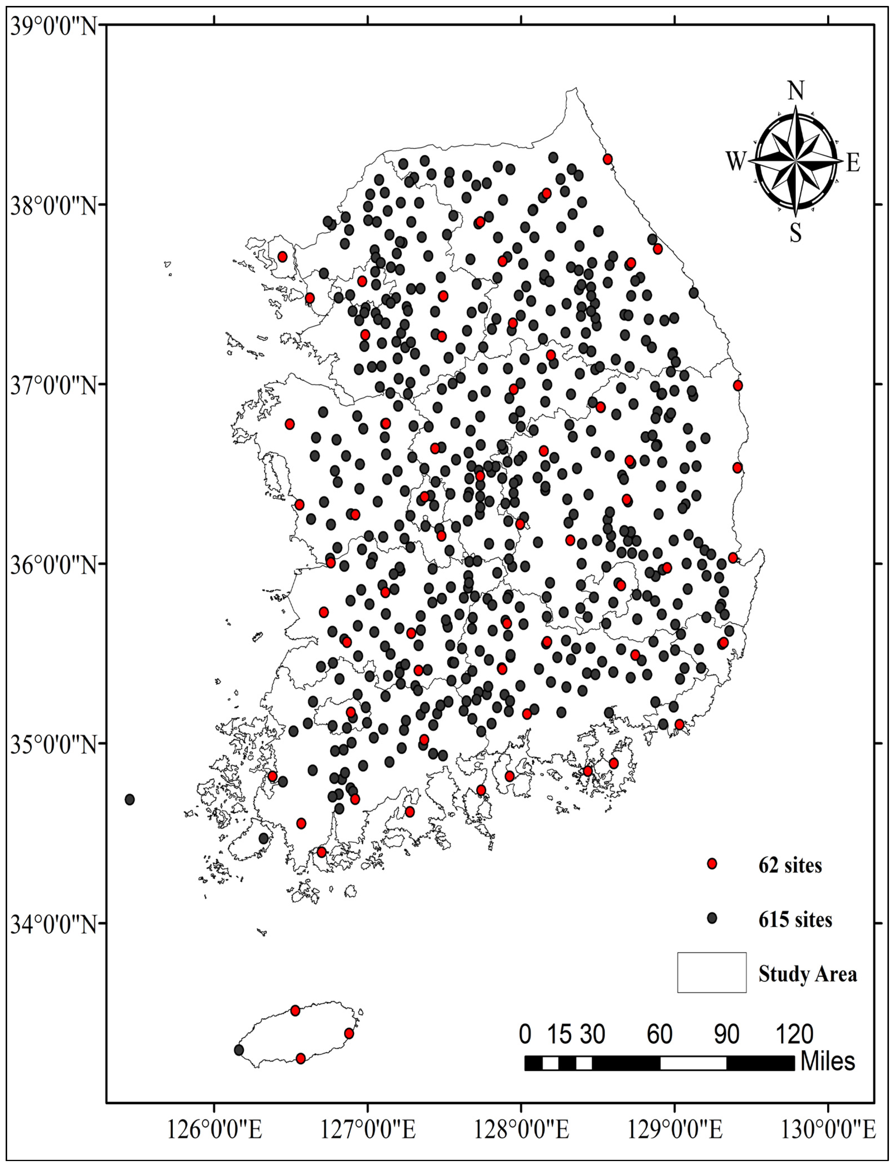
The study area covers the whole of South Korea, which spans across the five major rivers including Han-gang, Nakdong-gang, Geum-gang, Yeongsan-gang, and Seomjin-gang river basins and their tributaries. The management of precipitation data in Korea is conducted in a systematic manner. Recently, a standard report has been published about the hydrological process, and suggested 615 representative sites for the estimation of rainfall quantile [30]. Figure 1 shows the study area and 615 sites, including 62 sites (highlighted in red dots) that have been operated for more than 40 years.

2.2. Datasets

The observed rainfall data were managed by Korea Meteorological Administration (KMA), Korea Water Resources Corporation (K-water), and the Korean Ministry of Environment (MOE), and the all observed datasets were acquired from the water resources management information system (WAMIS, http://www.wamis.go.kr/, accessed on 13 February 2023). In this study, the 615 sites were selected to calculate SPMPs and compare them with the HPMP for the 2020 historical period. Notably, in previous studies conducted in South Korea [10,11,31], the HPMP was calculated for the 62 sites, using more than 40 years of rainfall data. Therefore, the present study involved the calculation of SPMPs for a total of 615 sites, and results were compared with those obtained for results of HPMPs [10] which had been conducted for 62 sites.

The previous study reported that the HadGEM3-RA (12.5 km resolution) model appropriately simulated the statistical characteristics of annual maximum (AM) precipitation data [32]. In addition, several studies applied the HadGEM3-RA model to estimate the quantitative change for a future period [11,33]. In particular, Lee and Kim [11] projected the future HPMP based on the RCP4.5 and RCP8.5 scenarios. Therefore, the future SPMPs were estimated and analyzed for RCP 4.5 and 8.5 scenarios and the 2100 future period. The HadGEM3-RA climate model developed by the KMA was applied to estimate the future precipitation data because it is the most commonly used model in South Korea. The simulated precipitation data of HadGEM3-RA can be accessed through the climate information portal (CIP, http://www.climate.go.kr/home/, accessed on 13 March 2023) website.

The SPMPs were calculated by dividing them into three spans (2040, 2070, and 2100) for the future period, as listed in

Table 1. Classification of future scenarios.

Climate Scenario	Period (Year)
RCP 4.5 and 8.5	Obs. start year~2040
	Obs. start year~2070
	Obs. start year~2100

. The estimated SPMP values were compared with the HPMP for 62 precipitation sites, which were provided for HPMP (2100) in South Korea (red dots in Figure 1) [10].

3. Methodology

3.1. Hershfield Method

The hydrometeorological method and statistical method are commonly applied methods for PMP estimation. Hershfield [15] proposed the PMP estimation method based on the frequency factor [29], as shown in Equation (1):

$${\mathrm{P}\mathrm{M}\mathrm{P}}_{24}={\overline{X}}_n+K_M\times S_n$$

(1)

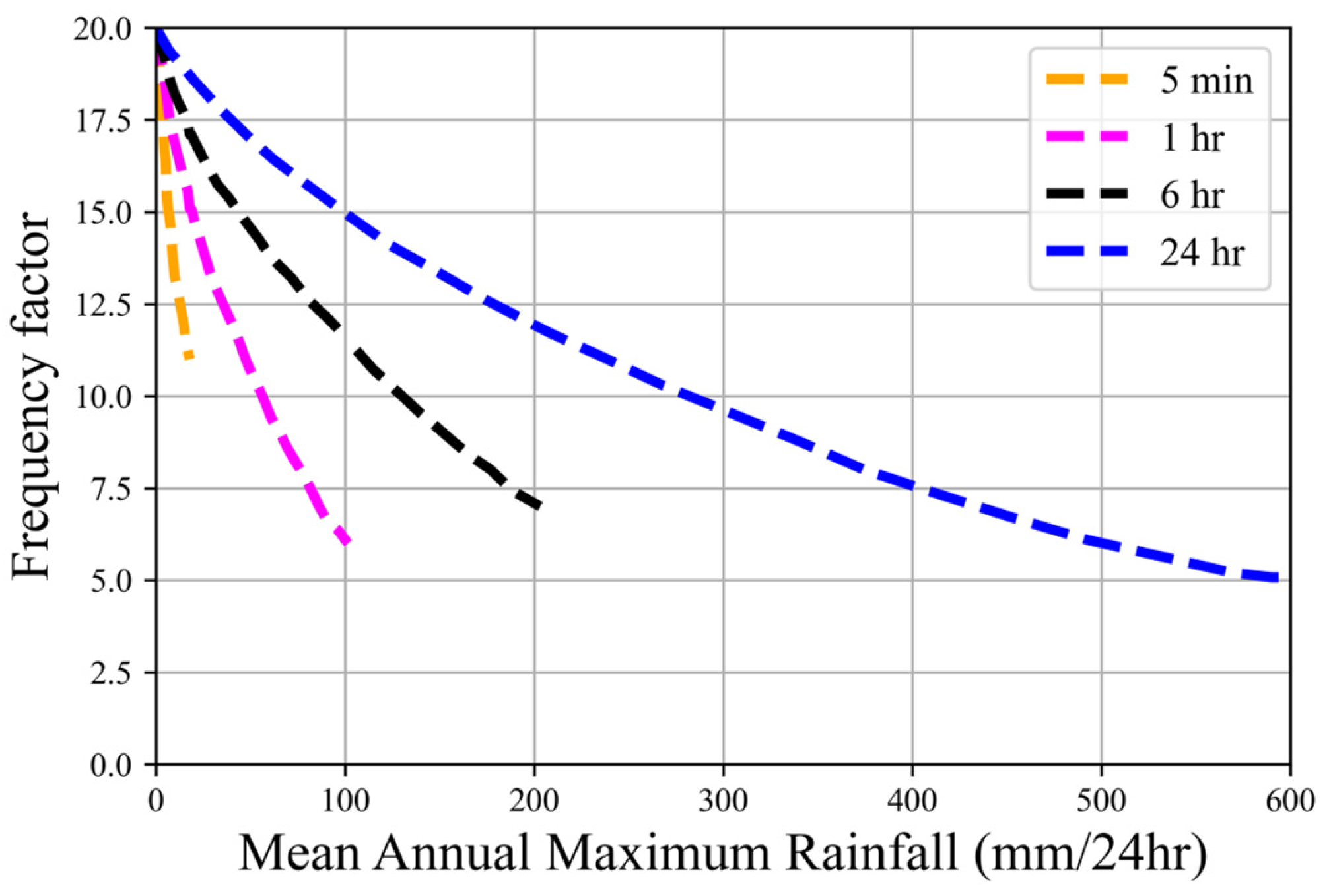
where ${\mathrm{P}\mathrm{M}\mathrm{P}}_{24}$ is the estimated $\mathrm{P}\mathrm{M}\mathrm{P}$ (mm) based on precipitation data (24 h); ${\overline{X}}_n$ and $S_n$ are the mean and standard deviation of annual maximum precipitation, respectively; and $K_M$ is the frequency factor, which can be calculated using Equation (2). Hershfield [15] initially suggested a fixed value of 15 ($K_M=15)$: however, a subsequent study [28] demonstrated that the fixed value of 15 may be too high and low, respectively, for regions with high and low annual rainfall. Therefore, Hershfield revised a $K_M$ value of between 5 and 20, based on the nomograph, as shown in Figure 2.

$$K_M=\frac{X_{max}-{\overline{X}}_{n-1}}{S_{n-1}}$$

(2)

where $X_{max}$ is the maximum precipitation of the observed data and ${\overline{X}}_{n-1}$ and $S_{n-1}$ represent the mean and standard deviation of the annual maximum precipitation, except $X_{max}$, respectively.

3.2. Hershfield’s Nomograph

In this study, the frequency factors of the 615 sites were calculated using the Hershfield’s nomograph (=envelope curve). The WMO [1,2] proposed a frequency factor for 2600 weather stations covering 90% of the entire United States. The rainfall frequency factors of the correlations suggested by the WMO [1,2] are herein presented for each duration (5 min, 1 h, 6 h, and 24 h), and the frequency factor can be calculated using the average rainfall for each duration. Notably, $K_M$ is a function of rainfall duration and mean annual rainfall, as shown in Figure 2.

3.3. Frequency Factor Method

Chow [29] proposed a frequency factor ($K_T$) for computing the quantile for a given return period, $T$ (=return period) as presented in Equation (3):

$$x_T=\overline{X}+K_T{S}_X$$

(3)

where $\overline{X}$ and $S_X$ are the mean and standard deviation for the given data, respectively. For example, the cumulative distribution function of the general extreme value (GEV) model is given by the Institute of Hydrology [34].

$$F\left(x\right)=exp\left[-{\left(1-\frac{\beta \left(x-x_0\right)}{\alpha }\right)}^{1/\beta }\right]$$

(4)

where $x_0,\alpha >0$, and $\beta$ are the location, scale, and shape parameters, respectively. The frequency factor of the GEV model is given by

$$K_T=\frac{\left|\beta \right|}{\beta }\frac{\mathsf{\Gamma }\left(1+\beta \right)-{\left[-ln\left(1-\raisebox{1ex}{$1$}\!\left/ \!\raisebox{-1ex}{$T$}\right.\right)\right]}^{\beta }}{{\left[\mathsf{\Gamma }\left(1+2\beta \right)-{\mathsf{\Gamma }}^2(1+\beta )\right]}^{1/2}}$$

(5)

where $\mathsf{\Gamma }\left(·\right)$ is a complete gamma function. Moreover, the skewness coefficient of the GEV is given below:

$$\mathsf{\gamma }=\frac{\left|\beta \right|}{\beta }\frac{\mathsf{\Gamma }\left(1+3\beta \right)-3\mathsf{\Gamma }\left(1+2\beta \right)\mathsf{\Gamma }\left(1+\beta \right)+2{\mathsf{\Gamma }}^3\left(1+\beta \right)}{{\left[\mathsf{\Gamma }\left(1+2\beta \right)-{\mathsf{\Gamma }}^2(1+\beta )\right]}^{\frac{3}{2}}}$$

(6)

As shown in Equations (5) and (6), the frequency factor is a function of the return period and skewness coefficient, because the latter is only a function of the shape parameter and vice versa. In this case, the shape parameter is estimated based on the method of moments. Notably, the frequency factor of the three-parameter models is a function of the return period and skewness coefficient, whereas the frequency factor of the two-parameter models is only a function of the return period, because the skewness coefficient of the two-parameter models is constant (for example, the skewness coefficients for the normal and Gumbel distributions are 0 and 1.1396, respectively) [34].

3.4. Hydrometeorological Method

The hydrometeorological method is usually applied in practice in South Korea to estimate the PMP; it considers various meteorological variables, including precipitation data. The PMP estimation procedure using the hydrometeorological method is divided into five steps: identification of high-efficiency precipitation events, moisture maximization, storm transposition, data smoothing (envelopment), and PMP calculation for each duration from enveloped depth-area-duration (DAD) curves [31].

$$AP=R_{IP}\cdot R_{HT}\cdot R_{VT}\cdot OTF\cdot OP$$

(7)

where $AP$ is the adjusted precipitation, $R_{IP}$ is the moisture maximization ratio, $R_{HT}$ is the horizontal transition ratio, $R_{VT}$ is the vertical transition ratio, $OTF$ is the mountain transition ratio, and $OP$ is the observed precipitation. Lee et al. [31] expound the methodology and procedures of HPMP comprehensively. The observed precipitation here is assumed to be in a suppliable moisture state under ideal conditions, and becomes the moisture maximization ratio. In addition, the precipitation was transferred by considering the influence of mountains. Finally, after obtaining the adjusted precipitation for various precipitation events, the PMP can be obtained according to the duration and affected area [9].

In this study, the PMP Viewer program [10] was utilized for HPMP estimation, which was developed for South Korean practitioners. It estimates the HPMP based on observed precipitation data up to 2020, and the relevant meteorological variables. In addition, the future PMP values proposed by Lee et al. [31] were applied for the analysis. This study estimates the HPMP for the historical period of 2020, based on 615 sites. However, the HPMPs for the future period of 2100 were obtained from only 62 sites for RCP 4.5 and 8.5 scenarios, because these 2100 values were only available for 62 sites from the South Korea PMP report [31].

3.5. Statistical Measures

Several statistical measures were performed for the results of SPMPs to compare with the result of HPMP. The estimated SPMPs from the five methods were compared with the HPMP for 2020 using the mean absolute error (MAE), mean absolute percentage error (MAPE), root mean square error (RMSE), and SPMP/HPMP ratio. The equations of statistical measure are listed in

Table 2. Statistical measures and formulas for evaluating the results of SPMPs compared to the result of HPMP, where $n$ is number of observation sites, $x_i$ is HPMP value, and ${\widehat{x}}_i$ is SPMP value.

Statistical Measure	Formula
Mean Absolute Error (MAE)	$\mathrm{M}\mathrm{A}\mathrm{E}=\frac{\sum _{i=1}^n\left|x_i-{\widehat{x}}_i\right|}{n}$
Mean Absolute Percentage Error (MAPE)	$\mathrm{M}\mathrm{A}\mathrm{P}\mathrm{E}=\frac{\sum _{i=1}^n\left(\frac{\left|x_i-{\widehat{x}}_i\right|}{x_i}\right)}{n}\times 100\%$
Root Mean Square Error (RMSE)	$\mathrm{R}\mathrm{M}\mathrm{S}\mathrm{E}=\sqrt{\frac{1}{n}{\displaystyle \sum _{i=1}^n}{\left(x_i-{\widehat{x}}_i\right)}^2}$

.

4. Application and Results

4.1. Statistical Probable Maximum Precipitation for Historical Period

As previously stated, the objective of this study is to estimate and evaluate the SPMPs for both the historical (observed data up to 2020) and future period (simulated data up to 2100) in South Korea. Therefore, the five applied methods to calculate SPMPs were listed in

Table 3. Statistical methods for estimating the SPMP in this study.

Case	Statistical Methods
Case 1	$\mathrm{Hershfield}’\mathrm{s}\mathrm{fixed}\mathrm{frequency}\mathrm{factor}(K_M=15$)
Case 2	$\mathrm{Hershfield}’\mathrm{s}\mathrm{method}\mathrm{with}\mathrm{varying}{K}_M$ for each site
Case 3	Hershfield’s original nomograph
Case 4	Modified Hershfield’s nomograph
Case 5	Chow’s frequency factor method (T = 60,000)

. The SPMPs for Cases 1, 2, 3, and 4 were calculated using Equations (1) and (2) which include statistics (${\overline{X}}_n$, $S_n$) and $K_M$ values for each site. Moreover, Equation (3) was applied to calculate the SPMP for Case 5.

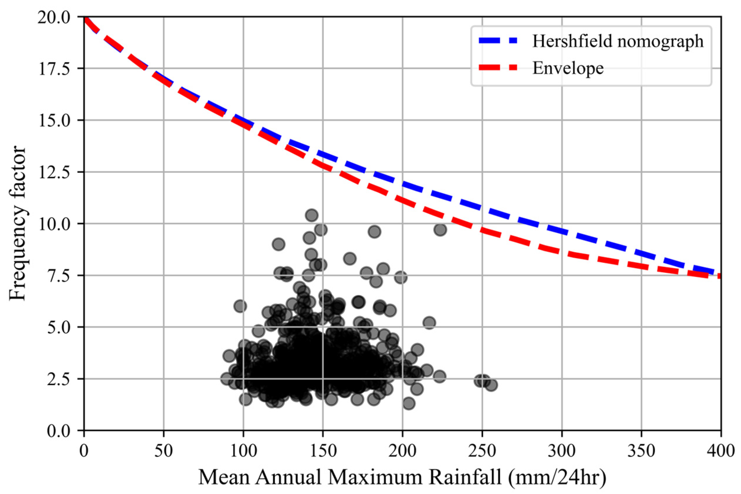
The blue line in Figure 3 is the graph originally proposed by Hershfield [28], and the red line is a graph enveloped by the modified Hershfield’ nomograph from 615 sites in South Korea. Hershfield’s original nomograph has the advantage of simplicity for calculating the SPMP. However, the nomograph using Hershfield’s envelope curve was derived for the United States, and may not apply to South Korea because of differences in rainfall characteristics. Therefore, this study was conducted using the data from 615 sites described in the Flood Design Standard Guidelines in South Korea [30]. In addition, the modified nomogram (representing “Envelope” in Figure 3) was derived from rainfall data of the study area, and is indicated in Equation (8).

$$K_M=6.4164\times {10}^{-5}\times P^2-5.6832\times {10}^{-2}\times P+20$$

(8)

where $P$ is the annual maximum daily precipitation (mm/24 h) and $K_M$ is the frequency factor.

In this study, the SPMPs were estimated by applying the five cases listed in

Table 4. MAE, MAPE, RMSE, SPMP/HPMP ratio, $K_M$, and SPMPs compared to HPMP (2020) for 615 sites.

Estimation of PMP		SPMPs					HPMP (2020)
		Case 1 Hershfield’s ${\mathit{K}}_{\mathit{M}} = 15$	Case 2 $\mathbf{Varying}{\mathit{K}}_{\mathit{M}}$ for Each Site	Case 3 Hershfield’s Nomograph	Case 4 Modified Nomograph	Case 5 Chow’s T = 60,000
PMP	Max.	2083	1420	1608	1719	2966	1396
	Mean	1035	357	909	955	1316	967
	Min.	395	141	403	411	437	598
$K_M$	Max.	15.0	10.4	15.4	15.8	35.1	-
	Mean	15.0	3.4	13.1	13.8	19.8	-
	Min.	15.0	1.3	9.7	11.0	9.7	-
Evaluation
MAE		184	613	150	149	372	-
MAPE		19	63	16	15	39	-
RMSE		249	634	194	189	487	-
SPMP/HPMP Ratio		1.071	0.369	0.941	0.988	1.361	-

, and the precipitation data up to 2020 for each site were used. In addition, the estimated SPMPs were quantitatively compared with the HPMP (2020) using the MAE, MAPE, RMSE, and SPMP/HPMP ratio. The SPMPs were estimated for 615 sites and compared with the HPMP (2020) because the HPMP could be obtained for 615 sites in South Korea [10].

The modified Hershfield’s nomograph (Case 4) shows the smallest average MAE, MPLE, and RMSE values, whereas the Hershfield’s original nomograph (Case 3) shows the second best among the applied methods, as shown in Table 4. The Hershfield’s method with varying $K_M$ for each site (Case 2) displays the worst results. In addition, the average SPMP/HPMP ratio of 615 sites for Case 4 shows 98.8% of HPMP (2020), with Case 3 showing the next closest ratio, as listed in Table 2. Case 2 yielded the smallest ratio, whereas Case 1 (Hershfield’s $K_M=15$) and Case 5 (Chow’s T = 60,000) achieved ratios greater than 1.0, which implies the average SPMPs are higher than the average HPMP (2020). Therefore, the SPMP of Case 4 was the closest to HPMP (2020), based on the assumption that the HPMP is the upper limit of PMP.

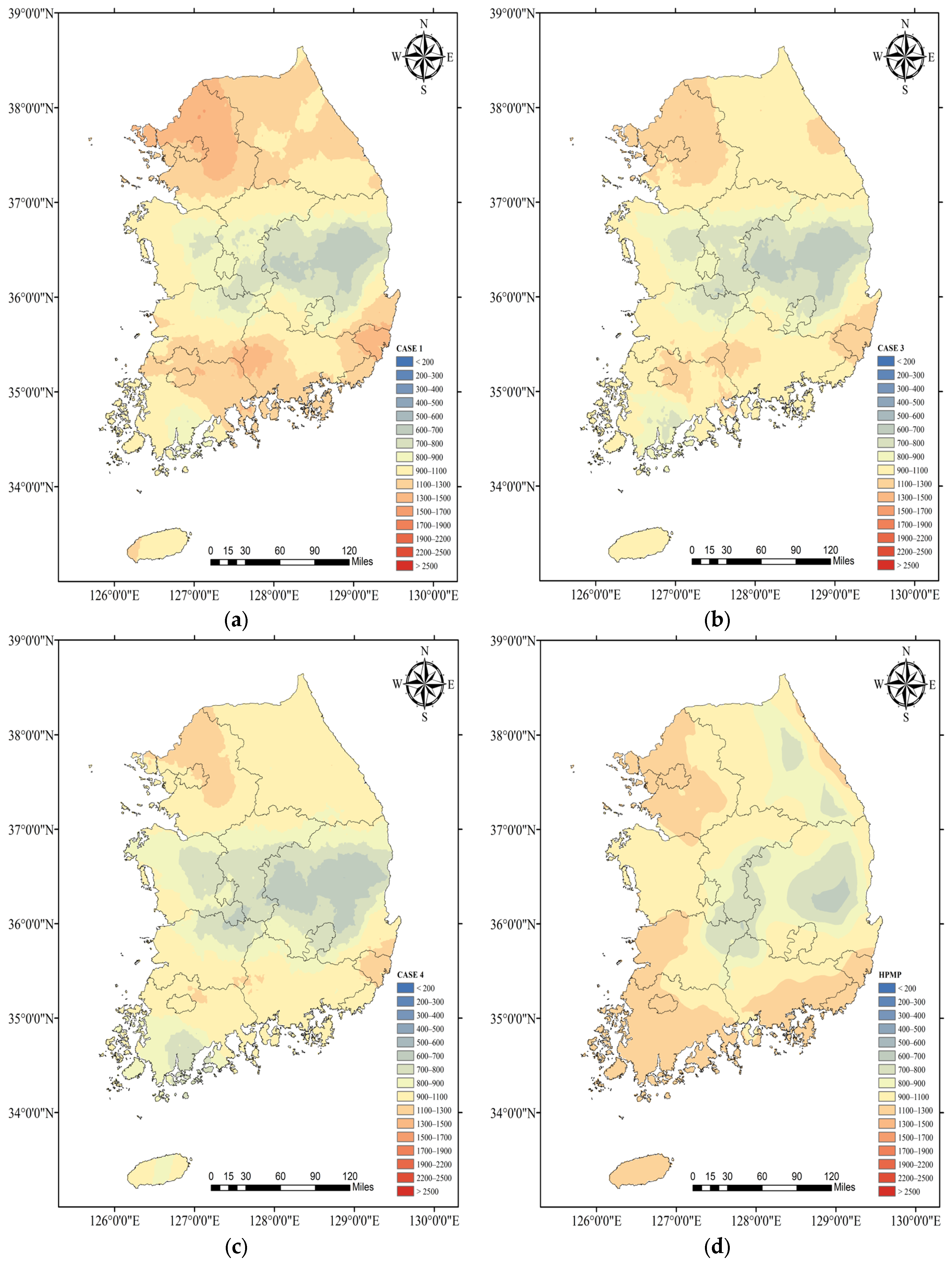
The spatial distribution of PMPs was conducted using the kriging technique. According to Table 4, Case 2 (Varying $K_M$ for each site) and Case 5 (Chow’s T = 60,000) shown that there are substantial differences compared to the results of HPMP, and these methodologies are indicated as not suitable for accurately estimating PMP in Korea. Therefore, the SPMPs (only the results of Case 1, 3 and 4) and HPMP for RCP 4.5 scenario of 2100 are presented in Figure 4. Figure 4 shows the kriging results of the SPMPs and HPMP for each case. Figure 4a–d show that the spatial patterns are similar even though their SPMP values differ in each case. However, regarding the HPMP, some regions exhibited different spatial patterns. In particular, the HPMP, unlike the SPMP, exhibited higher PMP values in the southwest and south coastal regions. Case 2 revealed overall smaller SPMP values, and Case 5 revealed larger SPMP values than other cases. For Case 2, the average value of $K_M$s for 615 sites was 3.4, which is considerably smaller than Hershfield’s original $K_M=15$, whereas the average $K_M$ for Case 5 ($\mathrm{T}=\mathrm{60,000}$ years) was 19.8, which is much larger than $K_M=15$. In addition, the average values of $K_M$s for Cases 3 and 4 were 13.1 and 13.8, respectively. Notably, Chow’s method was used to derive the frequency factor $K_T$ based on the GEV probability model, and a return period of 60,000 years was applied to Case 5 to estimate the SPMP, as suggested by Koutsoyiannis [20]. The SPMP of Case 5 exceeds the HPMP; therefore, the corresponding return periods of SPMP in South Korea are less than the 60,000 years suggested by Koutsoyiannis [20]. Applications of the five SPMP methods revealed that the modified Hershfield’s nomograph is the best statistical approach, compared with the HPMP for the 2020 historical period.

4.2. PMP of Modified Hershfield’s Nomograph for Future Period

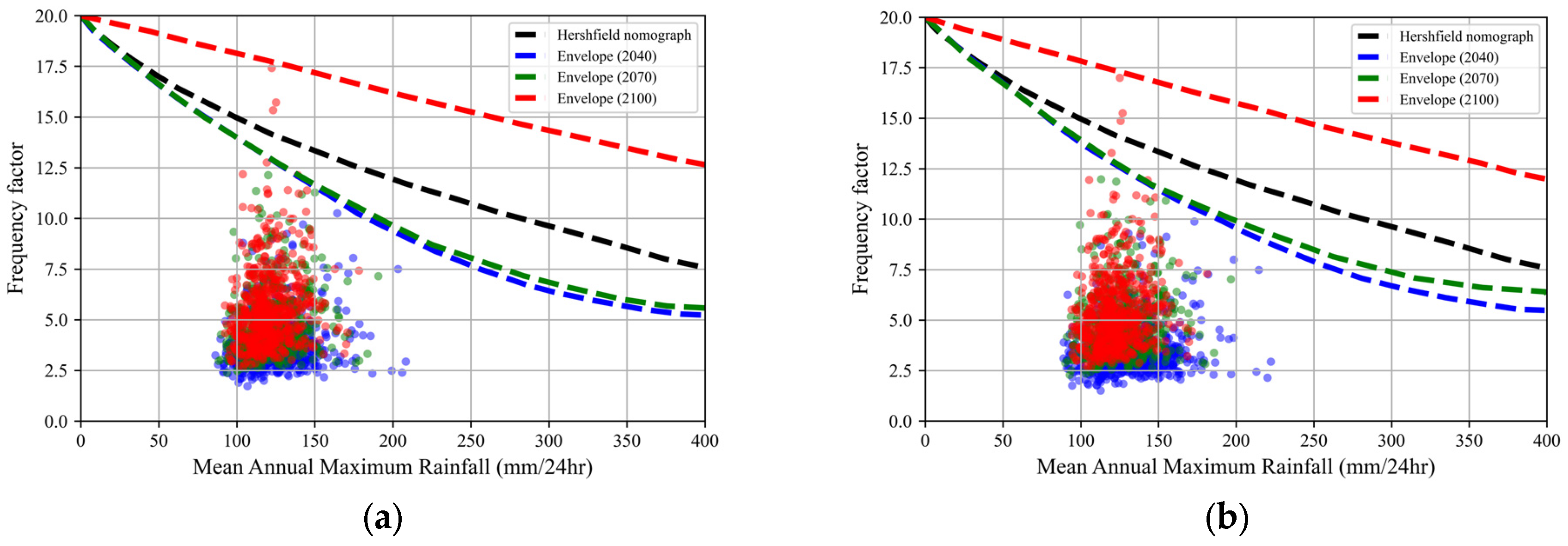
The modified Hershfield’ nomograph (envelope curve) was derived for each period and the RCP 4.5 and 8.5 scenarios in Figure 5. The frequency factors for each site have been computed and are represented by colored circles, with blue denoting the year 2040, green representing 2070, and red indicating 2100. As shown in Figure 5, the nomograph slopes for RCP 4.5 (left side) and 8.5 (right side) increased from 2040 (blue) to 2100 (red). Especially, both 2100 (red dashed line) periods show that the modified Hershfield’ nomograph (Case 4) has higher envelope curves than the Hershfield’s original nomograph (Case 3, dashed black line). Therefore, extreme maximum precipitations from 2070 to 2100 that affected the extremely high frequency factors can be inferred, and attributed to climate change, and the detailed results are summarized in

Table 5. Statistical information of SPMP (calculated using modified Hershfield’s nomograph, Case 4) based on RCP scenarios for future periods.

Scenario (Period)		RCP 4.5			RCP 8.5
		2040	2070	2100	2040	2070	2100
$K_M$	Max	16.5	17.0	25.5	16.6	17.0	25.0
	Mean	12.7	12.9	17.7	12.4	12.8	17.3
	Min	9.1	10.0	16.5	8.8	9.9	16.1
PMP	Max	1573	1904	2665	1810	1831	2614
	Mean	633	763	1079	788	779	1101
	Min	377	444	594	393	432	622

(even minimum values of $K_M$ in the period 2100 are larger than the Hershfield’s original $K_M=15$ for both RCP 4.5 and 8.5 scenarios).

Table 5 lists the statistical information regarding $K_M$ and the estimated SPMP using the modified Hershfield’ nomograph (Case 4) for RCP 4.5 and 8.5 scenarios and three future periods. As listed in Table 5, the maximum, mean, and minimum values of $K_M$ for the RCP 4.5 scenario are slightly larger than, or close to, those for the RCP 8.5 scenario. Furthermore, the minimum $K_M$ values for the period 2100 are larger than Hershfield’s original $K_M=15$ for both RCP scenarios. The frequency factor of $K_M$ increased as the future period shifted from 2040 to 2100, especially for the period 2100.

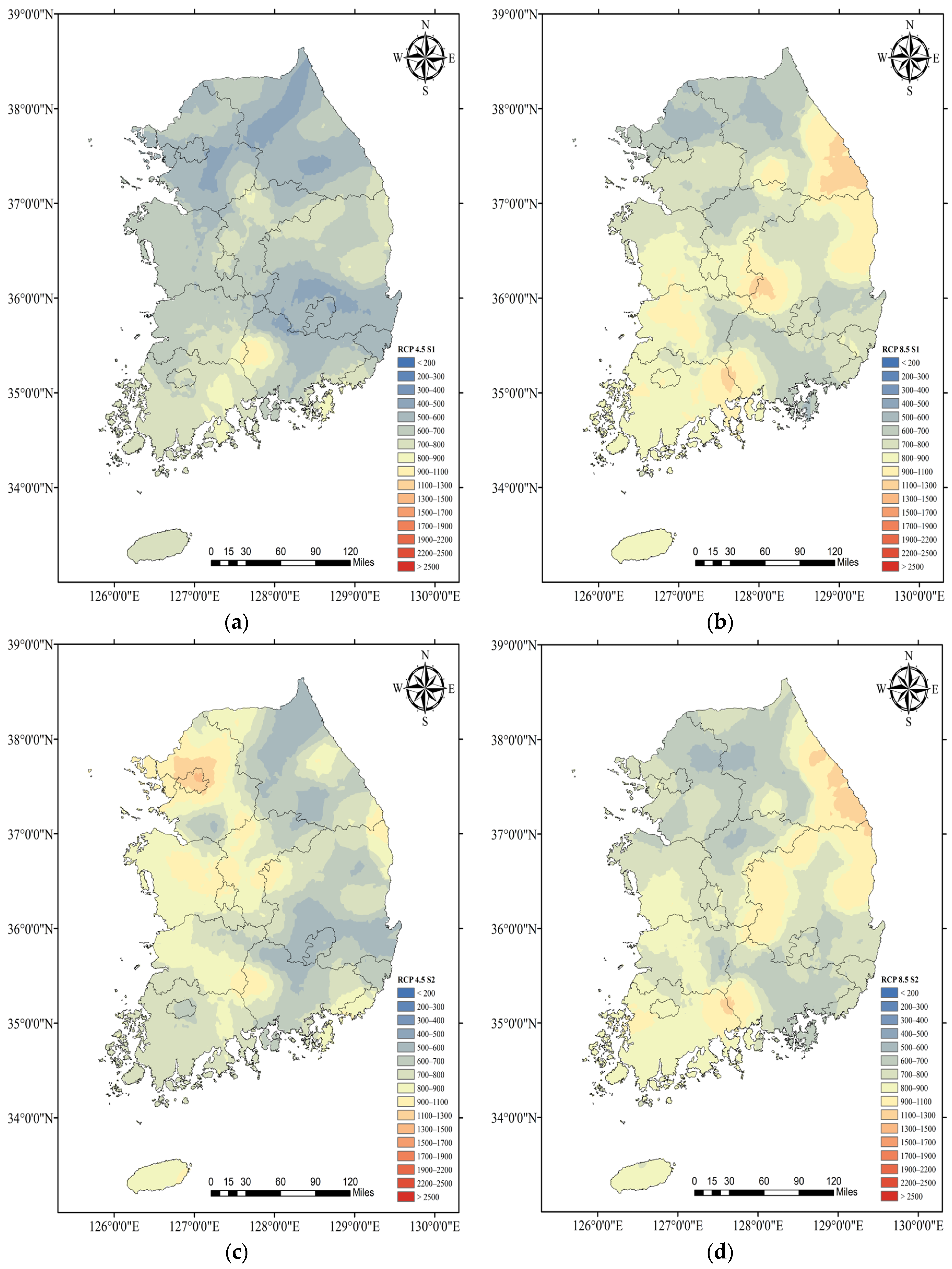
Figure 6 shows the contour maps of SPMP for each scenario and period using precipitation data from 615 sites. The SPMPs increased as the period was extended from 2040 to 2100 for both scenarios, even though their spatial distributions differed somewhat for each scenario.

4.3. Comparision of SPMP by Each Method for Future Period

The future SPMPs were compared with the HPMP for 2100. As mentioned before, the HPMP (2100) is only available for the 62 sites selected in South Korea [10]. Thus, the SPMPs for 2100 were estimated using only the future annual maximum precipitation data of the selected 62 sites for a fair comparison with the HPMP of 2100.

Table 6. MAE, MAPE, RMSE, SPMP/HPMP ratio, $K_M$, and SPMPs compared with HPMP (2100) for 62 sites.

Estimation of PMP			SPMPs					HPMP (2100)
			Case 1 $$\begin{gathered} \mathbf{Hershfield}’\mathbf{s} \\ {\mathit{K}}_{\mathit{M}}=15 \end{gathered}$$	Case 2 $\mathbf{Varying}{\mathit{K}}_{\mathit{M}}$ for Each Site	Case 3 Hershfield’s Nomograph	Case 4 Modified Nomograph	Case 5 Chow’s T = 60,000
RCP 4.5 scenario	SPMP	Max.	1823	1600	1643	2665	2795	1655
		Mean	967	480	948	1118	1361	1273
		Min.	514	172	535	599	611	856
	$K_M$	Max.	15.0	12.6	18.9	25.5	27.4	-
		Mean	15.0	4.9	12.6	17.7	18.5	-
		Min.	15.0	1.4	7.3	16.5	9.9	-
	Evaluation
	MAE		372	798	367	327	407	-
	MAPE		29	62	28	25	32	-
	RMSE		431	841	430	408	522	-
	SPMP/HPMP Ratio		0.760	0.377	0.745	0.878	1.069	-
RCP 8.5 scenario	SPMP	Max.	1968	1017	1828	2316	3634	2136
		Mean	1003	477	983	1137	1933	1566
		Min.	563	212	567	626	912	1019
	$K_M$	Max.	15.0	14.0	15.8	25.0	31.2	-
		Mean	15.0	5.9	14.8	17.3	24.0	-
		Min.	15.0	3.4	13.6	16.1	17.7	-
	Evaluation
	MAE		594	1089	605	512	514	-
	MAPE		37	69	38	32	34	-
	RMSE		646	1122	656	565	744	-
	SPMP/HPMP Ratio		0.641	0.304	0.628	0.726	1.234	-

lists the MAE, MAPE, RMSE, SPMP/HPMP ratio, $K_M$, and SPMPs of five cases based on the HPMPs (2100) for RCP 4.5 and 8.5 scenarios. The modified Hershfield’s nomograph (Case 4) exhibited the smallest MAE, MAPE, and RMSE values among the five applied methods, as listed in Table 6. In addition, the Hershfield’s method with varying $K_M$ for each site (Case 2) exhibited the largest MAE, MAPE, and RMSE values for both RCP 4.5 and 8.5 scenarios. Case 2 underestimated the SPMP because the estimated $K_M$s were relatively small, whereas Case 5 overestimated the SPMP because the corresponding return periods were less than 60,000 years in South Korea. These results are similar to those presented in Table 4.

The outcome presented in Table 6 bears resemblance to that of Table 4. As previously mentioned, Case 2 (Varying $K_M$ for each site) and 5 (Chow’s T = 60,000) are ruled out in Figure 7 and Figure 8, based on the findings of Table 6. For the RCP 4.5 scenario, Case 2 shows the overall smallest SPMP values, whereas Case 5 shows the largest SPMP values. For Case 2, the mean of the estimated $K_M$s for 62 sites was 4.9, which is considerably smaller than the Hershfield’s original $K_M=15$, whereas the mean of $K_M$ for Case 5 ($\mathrm{T}=\mathrm{60,000}$) was 18.5, which considerably exceeds $K_M=15$. In addition, the $K_M$s means for Cases 3 and 4 were 12.6 and 17.7, respectively. The Case 5 SPMP exhibits larger values than the HPMP in Figure 7d, suggesting that the corresponding return periods of SPMP are less than the 60,000 years suggested by Koutsoyiannis [20]: the average ratio was just above 1.0, as given in Table 6. For the RCP 8.5 scenario, Case 2 has the lowest SPMP values, while Case 5 has the highest SPMP values, which is similar to the RCP 4.5 scenario. For Case 5, the average ratio of 1.234 for the RCP 8.5 scenario was an increment from 1.069 under the RCP 4.5 scenario.

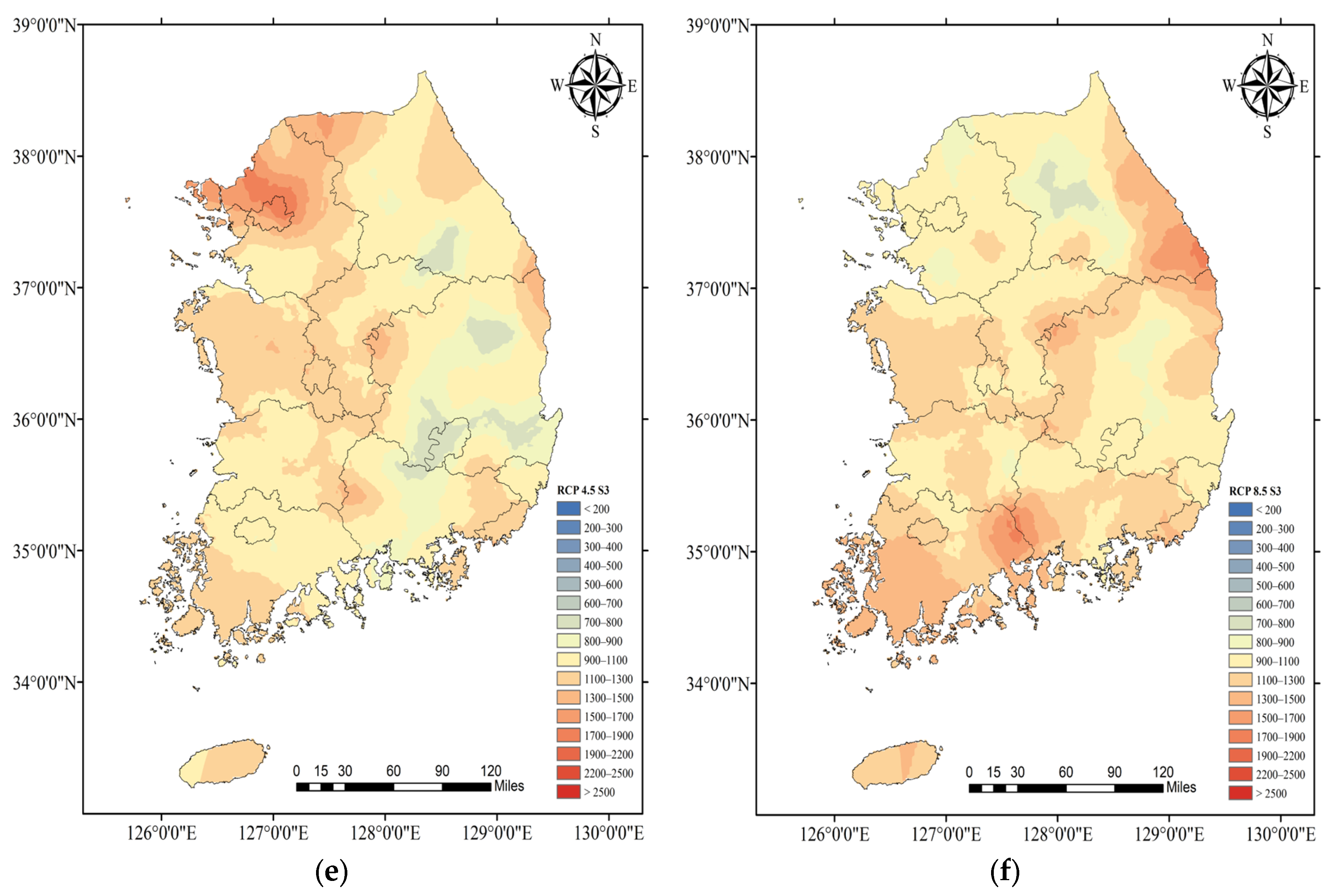
Figure 7 shows the result of SPMPs (except Case 2 and 5) and HPMP for the RCP 4.5 scenario of 2100. The kriging technique was employed to analyze the spatial distribution of PMPs, revealing distinct spatial patterns that differentiate SPMPs from HPMPs. For the RCP 4.5 scenario, the modified Hershfield’s nomograph (Case 4) was the best statistical approach compared with HPMP (2100): despite its SPMP being less than the HPMP (ratio = 0.878), it had a similar spatial distribution. Notably, the PMP in Figure 7c should be same as that in Figure 6e, but they have different PMPs with a similar spatial pattern because the PMPs in Figure 6e and Figure 7c were obtained from 62 and 615 sites, respectively. The SPMP in Figure 6e shows a detailed PMP spatial distribution, compared with the SPMP in Figure 7c.

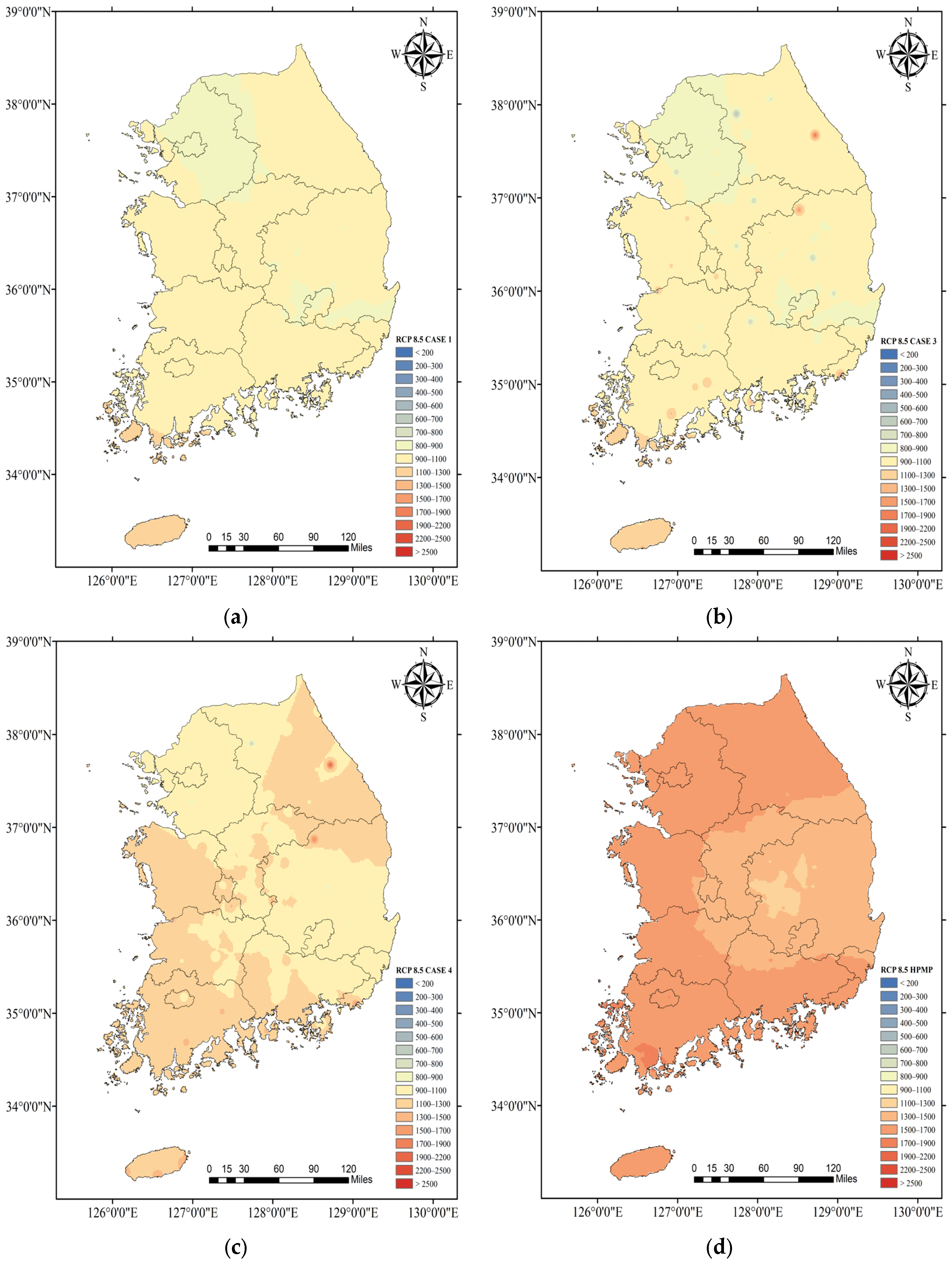
Figure 8 shows the spatial distributions of SPMPs and HPMP for the RCP 8.5 scenario of 2100. Among the statistical techniques employed, the modified Hershfield’s nomograph (Case 4) exhibited suitable performance in comparison to HPMP (2100), even though its ratio of 0.726 was smaller than the 0.878 for the RCP 4.5 scenario. In Case 4, the spatial characteristic of PMP represents the fact that the northwest and southwest coastal area is greater than the central inland, and this result is similar to that of the HPMP. Note that the PMP in Figure 8c should be the same as the PMP in Figure 6f, but they are a little different because the PMPs were obtained from 62 and 615 sites, respectively.

5. Conclusions

In this study, SPMPs are estimated using (1) Hershfield’s fixed frequency factor ($K_M=15$), (2) Hershfield’s method with varying values ($K_M$) for each site, (3) Hershfield’s original nomograph, (4) a modified Hershfield’s nomograph, and (5) Chow’s frequency factor method. The applied statistical methods are quantitatively evaluated, using the MAE, MAPE, RMSE, and SPMP/HPMP ratio. The estimated SPMPs are compared with the HPMP for historical (up to 2020) and future (up to 2100) periods for the RCP 4.5 and 8.5 scenarios, respectively. The conclusions obtained from this study are as follows.

For the historical period up to 2020, the estimated SPMPs were compared with the HPMP from 615 sites. The modified Hershfield’s nomograph (Case 4) was considered the best method, since it has the smallest MAE, MAPE, RMSE, and a SPMP/HPMP ratio of 0.988, whereas that of Hershfield’s original nomograph (Case 3) was the second best. In addition, the average SPMP/HPMP ratios of Hershfield’s fixed frequency factor ($K_M=15$) (Case 1) and Chow’s frequency factor method (T = 60,000, Case 5) are above 1.0. The ratio of Chow’s method is 1.361, which means that HPMP in South Korea is less than the 60,000 years suggested by Koutsoyiannis [20]. As a result, the modified Hershfield’s nomograph is the most appropriate method for estimating the SPMP among the five applied statistical methods.

The future SPMPs of 2100 estimated from the five statistical methods are compared with the HPMP of 2100 for the selected 62 sites and the RCP 4.5 and 8.5 scenarios. The HPMP values were only available for 62 sites in 2100, unlike the HPMP in 2020. The modified Hershfield’s nomograph exhibits the smallest MAE, MAPE, and RMSE, with SPMP/HPMP ratios of 0.878 and 0.726 for RCP 4.5 and 8.5 scenarios, respectively. Hershfield’s method with varying $K_M$ (Case 2) exhibits the worst results for both RCP scenarios, with ratios of 0.377 and 0.304, respectively. In addition, Hershfield’s original nomograph (Case 3) was the second best for the RCP 4.5 scenario but the second worst for the RCP 8.5 scenario.

The ratios of the Hershfield’s fixed frequency factor for the 2100 future period are 0.760 and 0.641 for RCP 4.5 and 8.5, respectively, whereas the ratio is 1.071 for the historical period of 2020. Thus, it is found that the Hershfield’s fixed frequency factor, $K_M=15$ is relatively large for the historical period but relatively small for the future period of 2100, due to climate change. Moreover, Chow’s frequency factor method (Case 5) shows ratios of 1.069 and 1.234 for RCP 4.5 and 8.5 scenarios, respectively. Thus, the return period of future SPMP of 2100 is less than 60,000 years, even when climate changes up to 2100 are considered. Finally, regarding SPMP estimation for historical and future periods, the modified Hershfield’s nomograph method (Case 4) was the appropriate statistical approach among the five statistical methods for estimating the SPMP in South Korea.

References

- World Meteorological Organization. Manual for Estimation of Probable Maximum Precipitation, 2nd ed.; Operational Hydrology Report No. 1, WMO, No. 332; World Meteorological Organization: Geneva, Switzerland, 1986. [Google Scholar]
- World Meteorological Organization. Manual for Estimation of Probable Maximum Precipitation; WMO-No. 1045; World Meteorological Organization: Geneva, Switzerland, 2009; ISBN 978-92-63-11045-9. [Google Scholar]
- King, L.M.; Micovic, Z. Application of the British Columbia MetPortal for estimation of probable maximum precipitation and probable maximum flood for a coastal watershed. Water 2022, 14, 785. [Google Scholar] [CrossRef]
- Gonzalez-Alvarez, A.; Coronado-Hernández, O.E.; Fuertes-Miquel, V.S.; Ramos, H.M. Effect of the non-stationarity of rainfall events on the design of hydraulic structures for runoff management and its applications to a case study at Gordo Creek Watershed in Cartagena de Indias. Colombia. Fluids 2018, 3, 27. [Google Scholar] [CrossRef]
- Johnson, K.A.; Smithers, J.C. Updating the estimation of 1-day probable maximum precipitation in South Africa. J. Hydrol. Reg. Stud. 2020, 32, 100736. [Google Scholar] [CrossRef]
- Ministry of Works. Estimation of Probable Maximum Precipitation in Korea: A Research Report on the Development of Water Resources Management Techniques; Ministry of Works: Seoul, Republic of Korea, 1988; Volume 3.
- Ministry of Land, Infrastructure and Transport. Estimation of Probable Maximum Precipitation in Korea; Ministry of Land, Infrastructure and Transport: Sejong-si, Republic of Korea, 2000.
- Ministry of Land, Infrastructure and Transport. Renewable Report of PMP Map in Korea; Ministry of Land, Infrastructure and Transport: Sejong-si, Republic of Korea, 2004.
- Ministry of Land, Infrastructure and Transport and K-water. PMP and PMF Calculation Procedure Guideline Establishment Service Report; Ministry of Land, Infrastructure and Transport and K-water: Sejong-si, Republic of Korea, 2008.
- Ministry of Environment. Re-Evaluation and Supplementary Research on Report the Probable Maximum Precipitation Calculation Procedure Report; Ministry of Environment: Sejong-si, Republic of Korea, 2020.
- Lee, O.; Kim, S. Estimation of future probable maximum precipitation in Korea using multiple regional climate models. Water 2018, 10, 637. [Google Scholar] [CrossRef]
- Beauchamp, J.; Leconte, R.; Trudel, M.; Brissette, F. Estimation of the summer-fall PMP and PMF of a northern watershed under a changed climate. Water Resour. Res. 2013, 49, 3852–3862. [Google Scholar] [CrossRef]
- Lee, K.; Singh, V.P. Analysis of uncertainty and non-stationarity in probable maximum precipitation in Brazos River basin. J. Hydrol. 2020, 590, 125526. [Google Scholar] [CrossRef]
- Micovic, Z.; Schaefer, M.G.; Taylor, G.H. Uncertainty analysis for probable maximum precipitation estimates. J. Hydrol. 2015, 521, 360–373. [Google Scholar] [CrossRef]
- Hershfield, D.M. Estimating the probable maximum precipitation. J. Hydraul. Div. 1961, 87, 99–116. [Google Scholar] [CrossRef]
- Lee, J.; Choi, J.; Lee, O.; Yoon, J.; Kim, S. Estimation of probable maximum precipitation in Korea using a regional climate model. Water 2017, 9, 240. [Google Scholar] [CrossRef]
- Desa, M.N.; Noriah, A.B.; Rakhecha, P. Probable maximum precipitation for 24 h duration over southeast Asian monsoon region—Selangor, Malaysia. J. Hydrol. 2001, 58, 41–54. [Google Scholar] [CrossRef]
- Sim, I.; Lee, O.; Jeong, S.; Kim, S. Estimating the return period for statistical probable maximum precipitation. J. Korean Soc. Hazard Mitig. 2019, 19, 373–382. [Google Scholar] [CrossRef]
- Sim, K.; Lee, O.; Kim, S.; Kim, E. Determination of minimum observation period for estimating probable maximum precipitation using statistical method. J. Korean Soc. Hazard Mitig. 2017, 17, 369–375. [Google Scholar] [CrossRef]
- Koutsoyiannis, D. A probabilistic view of Hershfield’s method for estimating probable maximum precipitation. Water Resour. Res. 1999, 35, 1313–1322. [Google Scholar] [CrossRef]
- Sarkar, S.; Maity, R. Increase in probable maximum precipitation in a changing climate over India. J. Hydrol. 2020, 585, 124806. [Google Scholar] [CrossRef]
- Hiraga, Y.; Iseri, Y.; Warner, M.D.; Frans, C.D.; Duren, A.M.; England, J.F.; Kavvas, M.L. Estimation of long-duration maximum precipitation during a winter season for large basins dominated by atmospheric rivers using a numerical weather model. J. Hydrol. 2021, 598, 126224. [Google Scholar] [CrossRef]
- Salas, J.D.; Anderson, M.L.; Papalexiou, S.M.; Frances, F. PMP and climate variability and change: A Review. J. Hydrol. Eng. 2020, 25, 03120002. [Google Scholar] [CrossRef]
- Rousseau, A.N.; Klein, I.M.; Freudiger, D.; Gagnon, P.; Frigon, A.; Ratté-Fortin, C. Development of a methodology to evaluate probable maximum precipitation (PMP) under changing climate conditions: Application to southern Quebec, Canada. J. Hydrol. 2014, 519 Pt D, 3094–3109. [Google Scholar] [CrossRef]
- Sarkar, S.; Maity, R. Estimation of probable maximum precipitation in the context of climate change. MethodX 2020, 7, 100904. [Google Scholar] [CrossRef]
- Rastogi, D.; Kao, S.-C.; Ashfaq, M.; Mei, R.; Kabela, E.D.; Gangrade, S.; Naz, B.S.; Preston, B.L.; Singh, N.; Anantharaj, V.G. Effects of climate change on probable maximum precipitation: A sensitivity study over the Alabama-Coosa-Tallapoosa River Basin. J. Geophys. Res. Atmos. 2017, 122, 4808–4828. [Google Scholar] [CrossRef]
- Kunkel, K.E.; Karl, T.R.; Easterling, D.R.; Redmond, K.; Young, J.; Yin, X.; Hennon, P. Probable maximum precipitation and climate change. Geophys. Res. Lett. 2013, 40, 1402–1408. [Google Scholar] [CrossRef]
- Hershfield, D.M. Method for estimating the probable maximum precipitation. J. Am. Water Works Assoc. 1965, 57, 965–972. Available online: http://www.jstor.org/stable/41264521 (accessed on 13 March 2023). [CrossRef]
- Chow, V.T. A general formula for hydrologic frequency analysis. Trans. Am. Geophys. Union 1951, 32, 231–237. [Google Scholar] [CrossRef]
- Ministry of Environment. Flood Design Standard Guidelines; Ministry of Environment: Sejong-si, Korea, 2019.
- Lee, O.; Park, Y.; Kim, E.S.; Kim, S. Projection of Korean Probable Maximum Precipitation under Future Climate Change Scenarios. Adv. Meteorol. 2016, 2016, 3818236. [Google Scholar] [CrossRef]
- Kim, S.; Shin, J.-Y.; Ahn, H.; Heo, J.-H. Selecting Climate Models to Determine Future Extreme Rainfall Quantiles. J. Korean Soc. Hazard Mitig. 2019, 19, 55–69. [Google Scholar] [CrossRef]
- Kim, S.; Joo, K.; Kim, H.; Shin, J.-Y.; Heo, J.-H. Regional quantile delta mapping method using regional frequency analysis for regional climate model precipitation. J. Hydrol. 2021, 596, 125685. [Google Scholar] [CrossRef]
- Institute of Hydrology. Flood Studies Report: Hydrological Studies, Volume No. 1; National Environment Research Council: London, UK, 1975; ISBN 978-09-01-87525-9. [Google Scholar]
Figure 1.
Study area and selected 615 sites including 62 sites (red dots show sites with rainfall data spanning more than 40 years) in this study.
Figure 2.
Nomograph of values based on mean annual maximum series and rainfall duration (Hershfield [28]).
Figure 3.
Nomograph of values based on mean annual maximum 24 h precipitation data from 615 sites. Hershfield’s nomograph (Case 3) is indicated in the blue dashed line, and the modified Hershfield’s nomograph (Case 4) is indicated in the red dashed line. The dots represent the frequency factor corresponding to mean annual maximum rainfall.
Figure 4.
Statistical and hydrometeorological probable maximum precipitation based on observed data up to 2020. (a) SPMP (Case 1, ); (b) SPMP (Case 3, Hershfield’s Nomograph); (c) SPMP (Case 4, Modified Nomograph); (d) HPMP (2020).
Figure 5.
Nomograph of frequency factor for RCP 4.5 and RCP 8.5 scenarios for future periods. (a) RCP 4.5; (b) RCP 8.5.
Figure 6.
SPMPs for Case 4 (modified Hershfield’s nomograph) for RCP scenarios and future periods 2040, 2070, and 2100. (a) RCP 4.5 (2040); (b) RCP 8.5 (2040); (c) RCP 4.5 (2070); (d) RCP 8.5 (2070); (e) RCP 4.5 (2100); (f) RCP 8.5 (2100).
Figure 7.
Statistical and hydrometeorological probable maximum precipitation using RCP 4.5 (2100). (a) RCP 4.5 (Hershfield’s ); (b) RCP 4.5 (Hershfield’s Nomograph); (c) RCP 4.5 (Modified Nomograph); (d) RCP 4.5 (HPMP).
Figure 8.
Statistical and hydrometeorological probable maximum precipitation using RCP 8.5 (2100). (a) RCP 8.5 (Hershfield’s ); (b) RCP 8.5 (Hershfield’s Nomograph); (c) RCP 8.5 (Modified Nomograph); (d) RCP 8.5 (HPMP).