
Deep Learning Approaches for Numerical Modeling and Historical Reconstruction of Water Quality Parameters in Lower Seine

M2C UMR 6143, CNRS, UNICAEN, University Rouen Normandie, F-76000 Rouen, France
*
Author to whom correspondence should be addressed.
Water 2023, 15(9), 1773; https://doi.org/10.3390/w15091773
Submission received: 12 March 2023
/
Revised: 14 April 2023
/
Accepted: 22 April 2023
/
Published: 5 May 2023
(This article belongs to the Special Issue Application of Machine Learning Techniques in Water Resources Management and Environmental Engineering)
Abstract
:Water quality monitoring is essential for managing water resources and ensuring human and environmental health. However, obtaining reliable data can be challenging and costly, especially in complex systems such as estuaries. To address this problem, we propose a novel deep learning-based approach that uses limited available data to accurately estimate and reconstruct critical water quality variables, such as electrical conductivity, dissolved oxygen, and turbidity. Our approach included two tasks, numerical modeling and historical reconstruction, and was applied to the Seine River in the Normandy region of France at four quality stations. In the first task, we evaluated four deep learning approaches (GRU, BiLSTM, BiLSTM-Attention, and CNN-BiLSTM-Attention) to numerically simulate each variable for each station under different input data selection scenarios. We found that incorporating the quality data with the water level data collected at the various stations into the input data improved the accuracy of the water quality data simulation. Combining water levels from multiple stations reliably reproduced electrical conductivity, especially at stations near the sea where tidal fluctuations control saltwater intrusion in the area. While each model had its strengths, the CNN-BiLSTM-Attention model performed best in complex tasks with dissimilar input trends, and the GRU model outperformed other models in simple monitoring tasks with similar input-target trends. The second task involved automatically searching the optimal configurations for completing the missing historical data in sequential order using the modeling task results. The electrical conductivity data were filled before the dissolved oxygen data, which were in turn more reliable than the turbidity simulation. The deep learning models accurately reconstructed 15 years of water quality data using only six and a half years of modeling data. Overall, this research demonstrates the potential of deep learning approaches with their limitations and discusses the best configurations to improve water quality monitoring and reconstruction.
1. Introduction
In the last century, many urban settlements have expanded extensively along rivers due to the availability and easy accessibility of water resources for human consumption and for agricultural and industrial activities. Unfortunately, this intensification of human activities in these sensitive environments has resulted in the release of various types of pollutants in dissolved and solid forms, leading to their environmental degradation [1]. Given the potential health and environmental risks associated with the use of contaminated water, environmental authorities have conditioned its use on compliance with certain quality standards [2]. These standards are generally established based on continuous and rigorous monitoring of a range of biophysical-chemical parameters of water to ensure that its use does not harm the ecosystem or human health [3]. To this end, environmental agencies have increased the number of hydrometric stations to monitor the qualitative and quantitative aspects of water bodies, although this task can be costly and technically challenging [4]. Indeed, environmental monitoring can be complex, requiring the simultaneous recordings of multiple variables (water level, temperature, electrical conductivity, pH, dissolved oxygen, turbidity, salinity) at several stations along the river to accurately capture water quality trends in response to climate variability and human practices [3]. Water resource management and protection may also involve the use of numerical models to better understand the natural and anthropogenic processes that control changes in water quality in long- or short-term [5,6]. The construction of numerical models is as important as the monitoring of environmental indicators in establishing strategies for exploiting and protecting the aquatic environment. This is because they provide decision-makers with relevant spatial information where there are no monitoring stations and indications of the impact of practices and hydraulic infrastructures on rivers before and after their implementation [7,8,9,10]. In the context of global climate change, these tools become indispensable to predict the hydrological impacts of climate change in the long term and to forecast extreme hydrological events (drought, floods).
In the literature, there are two main categories of numerical models: physics-based models and black-box models. Physics-based models are derived from physical laws in which the spatio-temporal distribution of concentrations of the substances of interest are determined by numerically solving a set of complex partial differential equations [11,12,13]. Since the transport processes of suspended or dissolved substances are governed by advection and dispersion phenomena, the mathematical formulation of the transport is expressed by two coupled equations that are solved sequentially [10]. The first one describes the hydrodynamics, where the spatial distribution of the flow velocity in the river is calculated and used in the transport equation to then simulate the concentration of the element of interest [14]. This kind of concept implies the use of a set of physical properties of the river, such as shear stress, bathymetry, and dispersion coefficients, which are generally variable in space, and their introduction are in simplified forms [15]. As is often the case, these transport equations ignore the multiple biophysical-chemical interactions that occur during particle transport. All these simplifications are sources of uncertainty added to the uncertainties associated with the boundary conditions used in the numerical solving of the hydrodynamic and transport equations [16,17,18].
Black box models, unlike physics-based models, are free of physical laws and therefore do not require the physical properties of rivers [5,19,20,21,22]. In this type of approach, the mathematical formulation relating the quality indicator under study (ex: dissolved oxygen) to the driving force variables (ex, River discharge) or with other geochemical variables (ex: salinity) used as inputs, is based on simple formulas [19]. In black box models using the concept of deep statistical learning, simple linear and nonlinear operations are performed sequentially on layers of neural networks to approximate highly nonlinear relationships between two or more variables. This approximation involves the identification of a set of matrices called weights and bias using the data available during the learning phase [23,24,25].
In recent years, models based on deep learning have been used widely in hydro-science applications, taking advantage of the development of a new type of neural network and the availability of large environmental databases. Indeed, the degree of uncertainty in the results provided by these models is related to the size of the database processed; the more data available, the more efficient the models become [26].
Most machine learning applications in hydrology have addressed the qualitative aspects of water bodies by performing numerical simulations to determine the discharge rate, streamflow [27], or water level of rivers. However, more and more, their use has been extended to qualitative aspects by relying on new neural network architectures. In that topic, we cite the recent work of Liu et al. [19] who built a predictive model of the Yangtze River (China) drinking water quality using the long short-term memory (LSTM) network to predict the following parameters: chemical oxygen demand (COD), NH3-N, pH, and dissolved oxygen (DO). The results of that study indicate the feasibility and effectiveness of using LSTM deep neural networks to predict the quality of drinking water in an IoT application, where the model input is the target variable. Barzegar et al. [28] proposed a hybrid network composed of a convolutional neural network (CNN) and an LSTM network to predict water quality indicators (dissolved oxygen and chlorophyll-a) in the small lake Prespa in Greece. The authors concluded that the hybrid CNN–LSTM models outperformed the standalone models (LSTM, CNN, SVR, and DT models) in predicting both DO and Chl-a, as this hybrid model successfully captured both the low and high levels of the water quality variables, particularly for the DO concentrations. This type of network was also chosen by Baek et al. [29] to simulate the water quality parameters of Nakdong River (total nitrogen, total phosphorus, and total organic carbon). Ubah et al. [30] applied the classical artificial neural network (ANN) to predict the water quality index of the Ele River (Nigeria) for irrigation at four stations. The ANN model succeeded in forecasting the water quality data where the model input is the target variable. Aldhyani et al. [31] applied and compared the effectiveness of several neural network algorithms (LSTM, nonlinear autoregressive neural network (NARNET), support vector machine (SVM), K-nearest neighbor (K-NN), and naive Bayes) to perform the tasks of prediction and classification of water quality parameters. In that study, the authors revealed that NARNET and SVM provide satisfactory results in prediction and classification, respectively. Jerry et al. [32] combined in situ punctual measurements of water quality parameters in Itasy Lake (pH, dissolved oxygen, conductivity, and turbidity) with remotely sensed imagery to establish a spatialized view of these parameters over the entire water body, using a dense neural network architecture.
In most previous works, numerical simulations of water quality parameters are based on the statistical processing of databases containing several sets of physicochemical variables collected over a long period of time. However, most rivers do not have a large database to easily apply deep learning tools, as is the case with the Seine River, which is the subject of this study. In the downstream section of the Seine, records of water quality parameters (electrical conductivity, dissolved oxygen, and turbidity) are limited compared to water level monitoring. However, historical analyses of water quality data along the Seine River are available in the literature [33,34], but mainly on a monthly scale in order to make long-term assessments of water bodies. Therefore, in this article, we explored the idea of using water level data to simulate hourly water quality parameters using neural networks. Thus, this strategy aims at linking hydrodynamic conditions and physico-chemical indicators, to reconstruct historical fluctuations of water quality parameters at some stations of the Seine where hydro-chemical probes were installed later than water level probes. Thus, unlike previous studies, this task is challenging as the target variable differs from the model input. In this work, we also test the relevance of the strategy by combining the analysis of water level data and physicochemical data to reconstruct historical physicochemical parameters. Furthermore, we study and discuss the effectiveness of latest generation deep learning networks in this quality data simulation task, such as GRU, BiLSTM, BiLSTM-Attention, and CNN-BiLSTM-Attention.
2. Material and Methods
2.1. Study Area and Data Acquisition
The hydraulic stations that are the subject of historical reconstructions of changes in water quality indicators are located in the downstream part of the Seine (Figure 1). In this estuary, the hydrodynamics and the physico-chemical properties of the water are under the pressure of oceanic, climatic, anthropic, and geological influences that vary according to the geographical position. In addition, the water quality in this region is impacted by multiple sources of pollution, including agricultural runoff, urbanization, and industrial discharges. As a result, water quality in the Seine River can be highly variable both spatially and temporally which make the modeling task more complex. Several sensors are placed in these stations to monitor the water level, electrical conductivity, dissolved oxygen, and turbidity. Our study utilized data from four monitoring stations located at varying distances from the sea, ranging from the closest to the farthest: Fatouville (estuary), Tancarville (mouth of the estuary), Val-des-leux (downstream), and Rouen (downstream). This choice of stations provides a better overview of trends in water quality indicators in the Lower Seine. They also allow to highlight the spatial and temporal correlations between the stations under the influence of various local forcings. At these stations, the recording of the water level started in 1990, but the measurement of the physico-chemical parameters started only in 2012. The stations in the estuarine zone, characterized by a strong oceanic influence, with a mega-tide whose amplitude can be up to 8 m, are equipped with two probes placed at two different depths to identify chemical stratification. The original raw data was recorded at an hourly scale, in order to capture the significant trends in tidal behavior that occur at the hourly scale and would have been lost if we had aggregated the data to daily intervals. The review of available data indicates that water levels are available from 1990 to the end of 2022. While water quality data is only available for the last few years, in some cases from January 2012 to 2022 and in other cases from May 2015 to 2022 (Figure 2). Thus, only six and a half years constitute the period of simultaneous record of water level and water quality parameters on which we can build a deep learning model. The data set is divided into two main parts: the first part of the data is used for training and validation of the model while the second part is used for testing. In this work, 70% of the available dataset is allocated to training, of which 20% is applied to the validation process in order to assess the adequacy of the generalization and avoid overfitting during the training process. The remaining 30% is used to test the model on new data to evaluate its effectiveness and reliability. However, not all available data periods can be exploited for some reasons: For the turbidity data, it turns out that the sensors have been replaced and this new sensor is calibrated differently, and the range of turbidity variation is not the same as the old sensor. For this reason, the simulation period is reduced to the period that was collected with the same sensor. In addition, the data for some parameters, such as electrical conductivity in the Val des Leux, are so noisy that we have discarded them.
2.2. Data Analysis
Before building the statistical learning models, we perform a correlation analysis of all variables to identify possible relationships between them and to evaluate the relevance of their use in the numerical modeling process. The topic of identifying and explaining interdependent relationships between water quality parameters in estuaries and with respect to their hydrodynamic conditions has been addressed in several papers [35,36,37,38]. Most of them have shown that the spatiotemporal trends of variables reflecting water quality exhibit strongly non-linear behaviors, which can be attributed to the concomitance of multiple influences of climatic, anthropogenic, and oceanic origin, whose intensities on the hydro-system vary spatially and temporally. This is demonstrated by the analysis of the annual variability of dissolved oxygen in relation to fluctuations in temperature and electrical conductivity of the water. Indeed, we observed that the oxygen content in the water column of the Seine increases with the decrease of the temperature during the seasons of low temperatures and oscillates also in the short-term during the diurnal and nocturnal periods (Figure 3 and Figure 4). In addition, heavy precipitation events occur during the cold season (between November and Mars), which further contributes to the enrichment of the Seine with oxygenated water. On the other hand, the intrusion of saltwater in the downstream stations, which are under the strong influence of the tides, especially with high coefficients leads to a depletion in the oxygen content of the water (Figure 3). The oscillations of mega tides are usually followed by the resuspension of sediments rich in organic matter, which in turn reduces the concentration of dissolved oxygen (Figure 3). Thus, an increase in turbidity and electrical conductivity is associated with a decrease in oxygen and can be seen in Figure 3 and Figure 4. However, the link between changes in electrical conductivity and turbidity, in general, is more complex to establish because changes in electrical conductivity are multifactorial and depend on the origin of the water. Our study of turbidity is limited to stations upstream of this area, where turbidity is triggered by high tide, which brings in salt water and causes an increase in electrical conductivity. In these environments, conductivity increases with turbidity, but with some time lag (Figure 3).
However, it is sometimes difficult to discern the characteristics of these relationships, especially in long records that include both long- and short-term effects due to the hydrological cycle and megatides. This point was revealed by the analysis of correlations presented in matrix form (Figure 5) in which, for example, the relationships between turbidity and water level or with other variables (dissolved oxygen and electrical conductivity) are difficult to detect on this time scale. This also concerns the correlations between electrical conductivity and water level acquired with the different stations in which the R coefficient is very low. On the other hand, high coefficients (−0.81 < R < −0.60) were found when correlating the electrical conductivity at river-dominated station such as Rouen and Val des Leux and the dissolved oxygen recorded at all stations. This coefficient is also significant at 0.74 < R < 0.91 when the time series of dissolved oxygen recorded at the different stations are correlated. For electrical conductivity, there are correlations only when the data from the two predominantly riverine stations (Rouen and Vals de Leaux) are compared with each other (R = 0.68), and the same is true for the predominantly oceanic stations (Tancarville and Fatouville, 0.6 < R < 0.9). On the other hand, correlations are weak when comparing electrical conductivity data recorded at one predominantly fluvial station and another dominated by the ocean.
In conclusion, the dendrogram alone may not provide sufficient guidance for the selection of inputs for subsequent modeling steps because linear correlation analysis is not sufficient to determine the presence or absence of dependencies among variables. Indeed, some dependencies may exist for some variables, but they are rarely linear and occur with some time lag. The relationship between a variable recorded at two stations may exist, but it is masked by the effect of tides and will not appear until that effect is removed. Thus, this analysis must be taken with caution. For this reason, we prefer to test multiple strategies in the selection of input variables. Additional statistical information on the available parameters is provided in Appendix A Figure A1, Figure A2, Figure A3 and Figure A4.
2.3. Nomenclature and Abbreviation
To avoid having large tables/figures in this paper, a simple abbreviation of the data name was necessary. For the water level data, the name for each station is the combination of WL and the first two letters of the station name: Water_Level_Caudebec = WLCa, etc. For the water quality data, the name for each case is the combination of the first letter of the quality type (C for electrical conductivity, D for dissolved oxygen, and T for turbidity), then the first two letters of the station name, then the location case (S for the surface and B for the bottom case). Table 1 recaps the nomenclature and abbreviation for later use.
2.4. Model Description
2.4.1. Models’ Architecture
In this study, we applied the following networks: GRU, BiLSTM, BiLSTM-Attention, and CNN-BiLSTM-Attention to predict water quality data and reconstruct its historical variations. The CNN and BiLSTM/GRU algorithms are among the most widely used deep learning algorithms and have been applied in various fields (e.g., image recognition and speech analysis) [39,40]. GRU and BiLSTM are widely used in processing sequential data such as time series [41]. CNN is known to be effective in image processing, especially in object and face recognition in photographs and movies [42]. However, CNN can also be adapted to the analysis of time series data by reformulating the problem into a 1D form or, if the time series are multivariate, can be processed as a 2D image. In the following subsections, we will describe in detail the properties and principles of these networks.
Long Short-Term Memory (LSTM)
The LSTM network was originally built by Hochreiter and Schmidhuber in 1997 [43] to avoid the gradient explosion and vanishing during the learning process of RNNs [44]. The LSTM designers added the forget gate, input gate, and output gate functions, to overcome the difficulties encountered in RNNs in the optimization phase called the backpropagation, which is used to identify the matrices (weights and bias) involved in approximating the relationship between the input and output variables. The structure of an LSTM cell is shown in Appendix A Figure A5. The LSTM model consists of several gates that control the flow of information into and out of the cell. The input gate determines how much of the input vector should be added to the cell state, while the forget gate determines how much of the previous cell state should be retained. The candidate value vector state is generated by the tanh activation function applied to the sum of the weighted inputs from the previous hidden state and the current input vector , and it is used to update the cell state . The output gate determines which information from the current cell state should be passed to the output, and the hidden state vector is generated as the element-wise product of the output gate activation vector and the hyperbolic tangent function applied to the current cell state . The equations for the LSTM model are as follows:
where , , , represent the weight matrices for the forget gate, input gate, candidate values, and output gate, respectively, and , , , represent the bias vectors for these gates that are learned during the training.
Bidirectional Long Short-Term Memory (BiLSTM)
BiLSTM is a network with a powerful architecture because it relies on the combination of forward and backward long-term memory (LSTM) for information retrieval [45]. The hidden state of the Bi-LSTM at the current time t contains both forward and backward hidden states. The conventional LSTM algorithm can only process time-related data in one direction. However, BiLSTM also incorporates inverse directional LSTM to capture the most important features that may be missed by LSTM. Therefore, BiLSTM greatly expands the amount of information available to the network for improving its predictive performance.
Gated Recurrent Unit (GRU)
GRU an improved variant of the LSTM algorithm, is known for its reliability in processing time series [46]. One of the main features of GRU is the inclusion of the forget gate and the input gate in the reset gate, as shown in Appendix A Figure A5. The reset gate deals with input and deletion of information, just like the input gate and the forget gate found in the classical LSTMs. The reset gate controls the amount of past data that must be discarded. Compared to the LSTM, GRU requires fewer parameters to be computed and processed. In addition, the hidden state is communicated directly between cells in the network, eliminating the need for an exit gate. This makes GRU easier to compute and implement, resulting in faster training times. The reset gate determines how much of the previous hidden state should be retained and how much of the current input should be added to the candidate hidden state . The candidate hidden state is computed by applying the activation function to the weighted sum of the previous hidden state and the current input multiplied by the reset gate . The output gate determines how much of the candidate hidden state should be passed to the output, and how much of the previous hidden state should be retained.
GRU network equations:
where , , and are the weight matrices for the output, reset, and candidate gates, respectively. , and are the bias vectors for the output, reset, and candidate gates that are learned during training.
Convolution Neural Network (CNN)-Based Bi-Directional Long Short-Term Memory (BiLSTM) with Attention Mechanism
The characteristics of the CNN-BiLSTM-Attention network tested in this work are shown in Appendix A Figure A5. This network consists of a combination of several layers, starting with CNN layers, followed by BiLSTM layers, all topped by an attention layer at the end, just before the output layer. The CNN layers are composed of convolutional layers that aim to extract useful features from the input data by sliding convolution kernels over this data. The extracted features are then injected into a BiLSTM. The output of the BiLSTM is then passed to the attention layer, which is discussed in more detail in the next section. A drop-out layer is then added to reduce complexity and avoid overfitting. To avoid neuron death and solve vanishing and gradient explosion problems, we add the rectified linear unit function (ReLU) as an activation function in the CNN layer [47]. Moreover, the sigmoid activation was included in the hyperparameter selection, so that the hyperparameter fitting process can select the optimal parameter.
Attention Mechanism
The basic concept of the attentional mechanism is inspired by human visual attention, according to which human vision can quickly detect and focus on critical information to capture more complete and relevant patterns. Attention is able to focus on some of the most important information in our dataset by weighting it and ignoring irrelevant information when building the predictive model [48,49].
The three stages of the attention process are presented in Appendix A Figure A5. The similarity score between Query and other keys variables’ values { is derived in the first phase, as indicated in Equation (11). There is only one method of calculating the score, which is based on the current state of the brain unit rather than its past state. It is a widely used method of calculating. The function is employed in the second phase to normalize the similarity score gained in the first phase, yielding the weight coefficient of each BiLSTM unit output vector, which is defined as Equation (12). The attention mechanism performs a weighted summation on the vector and the weight coefficient obtained in the previous phase to get the final attention values of each variable in the third phase, as shown by Equation (13).
where represents the similarity score of the Query to other keys variables, i indicates the serial number of variables, denotes the current moment, and , and stand for the output of Bi-LSTM layer, the weight matrix, and bias unit, respectively.
2.4.2. Model Evaluation Metrics
Evaluation of the performance of the trained deep learning models in terms of their effectiveness in reproducing the real data used in training or testing was conducted using 3 statistical evaluators: the root mean-square-error (RMSE), the relative RMSE (rRMSE %), and the coefficient of multiple determination ().
Root mean-square-error (RMSE):
The RMSE is the mean vertical distance of a data point from a fitted line. It effectively reveals huge differences and was thus utilized to establish prediction quality during the model learning phase. The RMSE equation is given as:
where is the real observed data, is the predicted data, and N is the number of samples.
The relative RMSE error metric “rRMSE”:
The coefficient of multiple determination (
):
In a multiple regression equation, the coefficient of multiple determination () indicates the proportion of variance in the dependent variable that can be predicted from the collection of independent variables. The equation is presented as:
2.4.3. Model Hyperparameters Tuning
The construction of the deep neural networks studied in this paper requires the use of several hyperparameters that must be selected before starting the training. In most cases, the tuning of these hyperparameters is based on the trial-and-error method, where several values are tested in order to keep only the best value in terms of its ability to provide a good fit to the real data in the training and testing phases. In this work, we used the Optuna library to define the range of these hyperparameters, where we sample their values in a stochastic optimization process to determine the optimal values [50]. For each model, a range of corresponding hyperparameter candidates has been reported in Table 2. To prevent overfitting and ensure the model’s ability to generalize well, the hyperparameters were tuned using the validation dataset, which was not used during training.
To train the deep learning models, Adaptive Moment Estimation (ADAM) stochastic optimizer was applied to minimize a loss function expressed as root mean square error (RMSE) [51]. The optimization algorithm is manually stopped when the network correctly predicts the training and validation data to avoid the overfitting problem [52]. Therefore, we chose a sufficiently large number of epochs (150 epochs) to ensure that a state of convergence is reached.
2.5. Modelling and Historical Reconstruction Approaches
The work presented in this paper consists of two tasks. The first task concerns numerical modelling, in which we establish the highly nonlinear relationships between these parameters (water level, electrical conductivity, dissolved oxygen, and turbidity) using neural networks by analyzing all the data recorded at the various stations along the downstream part of the Seine River. The networks created in the first phase of the modelling are then used in the second phase to carry out historical reconstructions of the quality parameters. However, this modelling is difficult to realize with limited and incomplete records to create a network with a good degree of generalization. To overcome this difficulty, a rigorous strategy was developed that involves searching for the best combinations of model input data and the best neural networks among (GRU, BiLSTM, BiLSTM-Attention, and CNN-BiLSTM-Attention) and their associated hyperparameters, as well as the targeted reconstruction order. In fact, the reconstructions of each variable will be sequential, so that the order of the target variables is predominant, as each completed variable serves as data to complete the next variable. Moreover, the complexity of the relationship between the variables under study varies, and some variables require the use of several intermediate variables to capture their evolution over time. Since the reconstruction of historical quality data can only be inferred based on water levels, which are the only parameter available over the reconstruction period, it is therefore necessary to sequentially incorporate previously reconstructed water quality data to recover the remaining quality parameters.
Several options were explored when selecting the inputs for the modelling part. For each target (conductivity, dissolved oxygen, and turbidity data), a set of features was chosen, such as: using only water level data from the same (or closest) station, using water level data from a set of surrounding stations, using water level data from all stations, using only water quality parameters, using jointly water level and water quality parameters from the same or closest station, combining water quality parameters and using the other part (bottom to surface and vice versa), and so on. In the process of selecting a neural network, we evaluated multiple networks through a thorough comparison to determine the optimal model for modelling and reconstruction. We analyzed and presented the performance of each network as the complexity of the task increased, starting with the most challenging task of using water level data to simulate water quality data. Our analysis study then moved on to simpler tasks, such as reconstructing water quality data using data from the same physical parameter at one station to simulate the same parameter at another station or at different stages (bottom and surface) within the same station, which may have a high correlation and be relatively simple to model. Different configurations in the choice of input data, network, and output parameter were tested using data available for the period (2015 to 2022). The quality of these simulations was expressed in terms of and rRMSE in matrix format and all the results were saved in a database. The analysis of these indicators was performed to determine the requirements for each step of the historical reconstruction, including the order of variables to be reconstructed, the selection of the appropriate model, and the best combination of inputs to optimize the reconstruction process. This strategy fills the selected target with the best model and hyperparameters used in this exercise, and the target feature is then added to the full features for subsequent feature construction. Figure 6 provides a visual representation of the historical reconstruction methodology.
Note that in modelling part, there is no restriction on feature selection because many models are tested with different input features. In contrast, in historical reconstruction, the data available at each step constrains the feature selection. For example, in the first step, only water level data from May 2014 to January 1990 are available for selection. Later, water quality data from a particular station (e.g., Electrical conductivity at Tancarville Bottom) will be available, expanding the feature selection for future reconstruction steps. The appropriate model developed in the modelling section will then be used. In summary, the goal of our work is not only to produce a numerical simulation and analyze the dependencies of water quality parameters, but also to perform a historical reconstruction where the choice of inputs is limited. The modelling phase is therefore used to demonstrate the performance of the model under a range of scenarios for each prediction objective and to create a database for the historical reconstruction step.
3. Results and Discussion
3.1. Modelling Task
In this section, the results of several input and target cases have been presented to investigate the possibility of inferring the data of a water quality parameter of a given station from the records of the other or same parameters of the same or other stations. In this analysis, we also investigate the suitability of predicting quality parameters based on water level variations, which is a readily available parameter from hydraulic stations.
The networks formed with the different configurations were tested with a small dataset due to the limited number of chronicles. The quality indicators of these networks are expressed by the average error of the model on the validation and test datasets, which allows us to better evaluate the degree of generalization of the networks. Both evaluation measures range from 0 to 100% for rRMSE, while values range from 0 to 1. We note that negative values can occur when the accuracy is very low, and the model does not match the target trend. In such cases, we can conclude that the selected input combinations do not match the target. Lower rRMSE values and higher values that are close to 1 indicate better accuracy.
3.1.1. Simulating Water Quality Parameters Using Only Water Level Data
In this section, we present the simulation results obtained by using water level data as input for determining the signature of the water quality parameters. These results are presented in Figure 7 and Figure 8 illustrate the overall test and the overall rMRSE test, respectively, for a range of configurations tested. Each figure comprises four subgraphs, each of which displays the results for a particular network indicated at the top of the subgraph. Each test result is shown in a block within the subgraphs and has a specific input selection on the x-axis and the corresponding target on the y-axis. The results of the four networks used in this work are presented.
We see from all these results that it is very difficult to predict the water quality parameters, especially the electrical conductivity at Fatouville (CFaB), using only the Honfleur water level as input, as shown by the low values that do not exceed = 0.49 with rRMSE = 22.26%. The accuracy of the prediction increased slightly when the water level of Tancarville was added as input, with the maximum value being 0.52 and rRMSE = 21.64% for the CNN-BiLSTM model Attention when predicting CFaB. However, adding Rouen water level as input showed better prediction accuracy in many cases (predicting CTaB, DFaB, etc.) for a set of model cases, such as GRU, BiLSTM, and BiLSTM Attention.
In addition, using a combination of many water level stations as input had a significant impact on prediction. Prediction of CFaB was possible with = 0.74 and rRMSE = 15.27% in the case of the CNN-BiLSTM Attention model and prediction of CTaB was possible with = 0.76 and rRMSE = 12.8% in the case of the BiLSTM model. However, not all additions of water level to the input combination had a positive effect on prediction. Some additions, such as adding the water levels of Honfleur and Tancarville (WLHo and WLTa) to the combination of the water levels of Duclair, Caudebec, and Rouen (WLCa_WLDu_WLRo), decreased the prediction accuracy in many experiments, such as the prediction of turbidity at Fatouville (TFaB) and the prediction of conductivity at Tancarville (CTaB). Thus, the WLCa_WLDu_WLRo input provided the most accurate prediction in a range of target cases. The degradation of the prediction accuracy when the water levels of the Honfleur station are included in the input data is due to the dynamics recorded at this station are only oceanic and do not include information on river dynamics, as is the case for the Seine stations. Therefore, the use of oceanic water level data can be considered as noise in the learning process. Thus, the best configuration for using water level data is to combine data from stations in the Seine River such WLCa_WLDu_WLRo that cover oceanic and continental forcings that affect variations in water level and water quality. We also note that the simulation of electrical conductivity at the stations near the sea (Fatouville and Tancarville) is relatively more accurate ( = 0.74 with rRMSE = 15.2 % and = 0.78 with rRMSE = 14.8% respectively) than at the Rouen station ( = 0.64 and rRMSE = 15.9%). However, in general, the reproduction of electrical conductivity at the different stations is feasible with the input water level data, unlike the simulation of turbidity and dissolved oxygen, which require the addition of other input parameters in the learning process. This suggests that water level data are more reliable and useful for predicting water electrical conductivity than other parameters.
3.1.2. Simulating Water Quality Parameters in Many Scenarios
In this section, we presented the results of water quality parameter prediction by adding water quality parameter data to the network inputs this time. In this framework, different scenarios of combining water level and water quality data are investigated. Moreover, for comparison purposes, the best input from the selection process of the last section using only water level data (WLHo_WLTa_WLRo) was included to get a complete overview of the simulation scenarios in terms of the type of input data. Figure 9, Figure 10 and Figure 11 illustrate the quality of the networks’ predictions in for the different data input scenarios (shown on the x-axis) and for the four networks tested. Each subplot is dedicated to a specific target mentioned at the top of the subplot. The purpose of these plots is to evaluate the predictive potential of water quality parameters (electrical conductivity, dissolved oxygen, and turbidity) at the three stations studied (Fatouville, Tancarville, and Rouen) based on water quality parameters and/or water levels. This also allows to evaluate the capabilities of the four models to predict water quality parameters in different situations, e.g., when monitoring the same water parameter at the same station (simple monitoring task such as predicting the next step of the same variable) or at different stations to study their interaction, or when simulating a water quality parameter using different parameters (from the same station or from different stations). In addition, we evaluate the effects of adding the water level data from the nearest station, as well as combining multiple water quality parameters when selecting inputs.
A first look at the results shows that the models are highly competitive with each other and in some cases give similar results. However, the results were sensitive to the choice of network and inputs, as shown by the differences in results when the inputs for the same target were changed (Figure 9, Figure 10 and Figure 11). Therefore, it is difficult to determine and generalize which model is the best for predicting water quality data without considering the specific input and target case. This is logical because each network has its own way of extracting trends from the data, and the performance of the model depends on the complexity, short-term, and long-term variations of the input data. However, it was observed that the highest prediction accuracy was achieved when the target parameters were among the input features. This means that using the existing records of a parameter in one period to predict its changes in neighboring periods is effective, regardless of the complexity of the target trend and the type of network. In this type of task, the GRU model has proven to be particularly efficient, especially when the features of the input and the target have similar trends. The ability of the GRU model to capture the fluctuating trends of different targets is shown in Appendix A Figure A6. It was observed that it is possible to simulate the electrical conductivity at the stations close to the sea (CFaB and CTaB) using the electrical conductivity data from the nearest station. However, it is difficult to accurately predict these values using only the Rouen electrical conductivity data, or the influence of ocean forcing on water quality is minimal. Adding the water level data from the nearest stations greatly improves the accuracy of the prediction in these cases. In addition, using the combined CRoS and DRoS data to predict CFaB and CTaB provides the most accurate results. Although the prediction of water conductivity at stations near the ocean is less accurate when only dissolved oxygen data are used, the addition of water level data from the nearest stations significantly improves the accuracy of the prediction. Predicting the electrical conductivity at Rouen station (CRoS) that is far from the sea, using only electrical conductivity data from CFaB and CTaB, stations near the sea (Fatouville and Tancarville), is not accurate (= 0.65 and rRMSE = 15.2%). This is because the stations on the mouth of the Seine are subject to sea intrusion, which is not the case of Rouen station. However, adding the water level data from the nearest stations to the electrical conductivity data from the nearest station significantly improves the prediction accuracy ( = 0.76 and rRMSE = 11.4%). The dissolved oxygen parameters for DFaB and DTaB, stations near the sea, showed a good ability to be used in simulating the dissolved oxygen parameter of the Rouen station (DRoS). When using the GRU model with only the electrical conductivity data from Fatouville, an of around 0.72 was achieved and rRMSE = 12.3%. When using both the electrical conductivity and dissolved oxygen data from Fatouville combined with the water level data from the nearest stations (WLHo_WLTa_WLCa_CFaB_DFaB), an of around 0.78 was achieved and rRMSE = 10.2%. It was also noted that using dissolved oxygen data at Tancarville (DTaB) as input to simulate water quality parameters at other stations is challenging. However, it is valuable in predicting its own value and the conductivity parameter at the same station. The CNN BiLSTM Attention model outperformed the other models in cases where they failed to capture trends in the input data, especially when the input data had complex or unusual patterns (e.g., when using DTaB alone to predict DFaB or CRoS). This indicates that the model is better suited to handle complex trends.
The results in Figure 10 clearly show that it is possible to predict the surface station data using the bottom one. In these cases, the GRU and BiLSTM models showed a high level of accuracy in predicting the water quality data (e.g., in the predictions of CTaS using CTaB, = 0.75 and rRMSE = 11.1%). Figure 11 suggests that it is possible to simulate the turbidity parameter using either electrical conductivity or dissolved oxygen data from the same station (e.g., predicting TFaB using CFaB or DFaB), with slightly better accuracy when using electrical conductivity data instead of dissolved oxygen data. However, a combination of water stations with electrical conductivity and dissolved oxygen data in the same input gave the highest accuracy. In addition, it was not possible to simulate the turbidity parameter at Fatouville using only electrical conductivity or dissolved oxygen data from a station far from the sea (such as Rouen station CRoS or DRoS). The BiLSTM network outperformed the other network when using only CFaB to predict TFaB. The BiLSTM-Attention model showed additional ability when adding a set of features, such as the water level, and combining CRoS and DRoS among the input. Meanwhile, the GRU outperformed other models when using local water quality parameters (electrical conductivity and dissolved oxygen at Fatouville) to predict the turbidity at the same station.
3.2. Historical Reconstruction
The numerical modelling task developed in the previous section allowed us, using the automated research process developed in Section 2.5, to determine the best configurations in terms of selecting the relevant input variables for each water quality parameter to be modelled and the most appropriate type of network to extract the relevant information from these data. These best configurations are shown in Table 3 and were used in the historical reconstruction of all quality parameters during the period (1990–2015) when only water level data were monitored without any high frequency monitoring of the quality aspects of the Seine. Table 3 also contains the evolution of the reconstruction steps, including the target to be filled in each step, the selected features from the available data, and the selected model.
Indeed, the reconstruction strategy is sequential, i.e., the variable reconstructed in first steps are used among input for the reconstructions of the following variables. Table 3 shows that it is best to reconstruct the conductivity and dissolved oxygen data before the turbidity data. This is due to the complexity of simulating a strong nonlinearity relationship such as turbidity from a single input variable. For this reason, the reconstruction is done from the combination of several input data. As for the bottom data, they are more reliable and less noisy and should be reconstructed before the surface data. In this way, the subsurface data can be used in reconstructions of surface data that are contaminated by noise. It is also worth noting that the combination of water level data and quality data gives effective results, so most variables were derived from this combination. Moreover, it is preferable to reconstruct the stations near the sea (Fatouville and Tancarville) before the other stations (Rouen and Val des Leux), because of the complexity of the trends of the latter and their short records. Indeed, variations in water quality parameters at stations close to the sea are mainly dominated by the tide, where the redundancy of semidiurnal fluctuations makes it easier for the network to extract the features of these variations. This is very complex to achieve at upstream stations which are under the influence of the hydrological cycle with complex low frequency trends. In addition, by analyzing the chosen models in the historical reconstruction steps (Table 3), our analysis revealed that the CNN-BiLSTM attention model was selected for most of the complex reconstruction tasks, particularly when the input data differed significantly from the target. The model’s success can be attributed to its ability to extract local features using convolutional layers, capture long-term dependencies in the input sequence using bidirectional LSTM layers, and focus on relevant input features using the attention mechanism. Furthermore, we found that the GRU model was selected and demonstrated strong performance in simpler reconstruction tasks steps where some input contains some features that share similar trends with the target feature (e.g., reconstruction of the dissolved oxygen at Val_Des_Leux (DVaS) using the same water quality parameter at Rouen (DRoS)). This is due to its simpler architecture with fewer parameters that can be advantageous for simpler input-output relationships. Our results highlight the importance of choosing an appropriate model based on the input data characteristics and the complexity of the reconstruction task.
In Figure 12, the simulation evaluation results for certain historical reconstruction steps are presented, while the historical reconstructed parameters for specific stations can be visualized in Figure 13. In addition to the historical reconstruction, we have made several corrections to the original data that are contaminated with noise whose values do not correspond to reality, such as the electrical conductivity data at Val-des-Leux (as shown in Figure 12—Step 8).
The quality of the numerical reconstructions is evaluated qualitatively by comparing the trends in the simulated data with the acquired data and quantitatively by using some historical dissolved oxygen data acquired in irregular and low frequencies in areas near the Rouen and Tancarvilles stations. Qualitative trend analysis in the reconstructed records shows that the short- and long-term variations in water quality parameters at all stations exhibit some physical consistency, such as that observed in the available data and described in Section 2.2. For example, at the Rouen station, during the period 1993–1996 (See Figure 14), we retrieved in the reconstructed records the seasonal cycle in the fluctuations of electrical conductivity and dissolved oxygen, characterized by a decrease in electrical conductivity and an increase in dissolved oxygen during the rainy months, consistent with the enrichment of the hydro-system with highly oxidized and less conductive water. These types of fluctuations have been recurrently noted in the available data plotted in the Figure 4. Reconstructed signatures of turbidity, dissolved oxygen, and electrical conductivity at stations with tidally influenced water quality such as Tancarville confirm this relationship as well as the interdependencies between variables discussed in the data presented in the Figure 15.
The reconstructed water quality data in Figure 14 and Figure 15, which cover the period from 1993 to 1997 at Rouen, and 1991 to 2004 at Tancarville, respectively, serve as a valuable tool for evaluating the reliability of the model’s historical reconstruction from a physical correlation perspective. The reconstructed parameters display a strong adherence to the logical physical relationships among the various water quality parameters, such as conductivity, turbidity, and dissolved oxygen. For instance, an increase in conductivity typically results in a decrease in dissolved oxygen, which is evident in the reconstructed data.
For the quantitative analysis of the quality of the historical reconstruction, we used a raw data set from the NAIADES-Eau-France database. These data are collected at low frequency and irregularly, sometimes with 2–4 measurements per year, as well as in areas different from those where the high frequency data acquisition sensors used in the present study are installed. Therefore, these differences in data collection prevent a comparison between the two types of measurements, as shown in Figure 16, which illustrates the differences in their evolutions during the period 1990–2020. For this reason, we limit this comparison to the identification of general trends in the magnitude of the fluctuations, especially for dissolved oxygen. In fact, over the period (2015–2019) for which data are available, the low-frequency measurements at Rouen as well as at Tancarville are well within the range of variation of the high-frequency data (Figure 16). This is also true for the variations of the reconstructed data with those of low frequency over the period (2000–2015). However, for the period prior to 2000, we observe that the reconstructed data have a different trend from the base frequency data, characterized by an overestimation of dissolved oxygen values compared to the low-frequency data. This difference is due to the fact that the recent learning data are acquired in a physico-chemical context that favors an oxygen enrichment of the waters that is completely different from the one that precedes the 2000s, marked by an oxygen deficit. This change has been identified in previous work carried out on the Seine [53], in which an improvement in water quality was noted following the implementation of a policy of creating treatment plans for urban waste. Thus, for the period before 2000, the uncertainty of the reconstructions is very high because the data used for training do not capture the physical-chemical conditions of this period affected by highly polluted urban rejects, which is one of the limitations of deep learning tools. Thus, we recall that the quality of generalization of the predictions with these tools depends on the amount of training data and on the nature of their characteristics.
For further reconstruction validation, especially on short-term scale, we compared our dissolved oxygen reconstructed data with reference data collected by the Seine aviation service and presented in the work of Le Pichon et al. [34]. The reference data were collected at a monthly scale, which limits our ability to validate our results on an hourly scale. Nonetheless, we calculated the monthly mean values for the year 2010 as presented by Le Pichon et al. [34] and used these values to assess the accuracy of our reconstructed data. This approach provides an additional means of validation for our dissolved oxygen reconstruction and supports the robustness of our results. Figure 17 illustrates this comparison. It can be seen that our reconstruction respected the overall trends in behavior across the year 2010 with high R2 = 0.813 in the case of Rouen and R2 = 0.814 in the case of Tancarville. The mean monthly values are close to the reference at the beginning and end of the year. However, some low robustness appeared in simulating the end of the summer season, especially in the case of Rouen.
4. Conclusions and Future Works
The objective of this paper is to evaluate the deep learning models’ effectiveness in numerically simulating water quality parameters (electrical conductivity, dissolved oxygen, and turbidity) at several surface and bottom stations located in the downstream section of the Seine. The study aims then to reconstruct the historical data of these parameters for a period of 25 years (January 1990 to January 2015). At these stations, the water level as well as the quality parameters are the result of the concomitance of multiple climatic, oceanic, geological, and anthropogenic factors whose degree varies from station to station. However, the variations of the quality parameters can be sorted into groups, one predominantly oceanic and the other predominantly fluvial, and even the water level fluctuates with the tide in all stations. The study consists of two tasks, numerical modeling and historical reconstruction. Numerical modeling involved finding the optimal configuration to numerically simulate each variable for each station. The optimal configuration is obtained from the tests of various input selection scenarios, where the water level and water quality data recorded at different stations are used individually or jointly in these tests to form the networks. In addition, we tested four networks with different architectures. In the end, the optimal configurations for each variable in terms of input data type and network types were selected to reconstruct the missing historical data in the second task. In that process, we concluded these following points:
- ✓
- The classical correlation analysis used to decrypt the relationships of interdependence between the parameters involved in this study does not allow us to identify clear relationships due to the strong nonlinearity that links them.
- ✓
- Training DL networks to reconstruct variations in water quality parameters based on water level has been shown to be effective, particularly in predicting electrical conductivity at stations located near the sea. This is because of the strong correlation between water level and increasing or decreasing seawater intrusion during tide oscillations. However, at predominantly fluvial stations, the water level data are not sufficient to simulate the electrical conductivity.
- ✓
- Reconstructing a water quality parameter for a given station using a network trained with the same parameter but collected at other stations proves to be an effective solution, especially when the data from the stations used are subject to the same environmental influences.
- ✓
- Deep learning tools are also powerful in identifying temporal interdependencies of each parameter to accurately predict missing data using available historical data. While our initial results using a small modelling data period are promising, it is important to consider that this approach may require longer records and additional parameters, including meteorological data, TSS, TDD, Chloride, etc., to achieve even greater accuracy and more reliable reconstructed data. Therefore, future studies should explore the potential benefits of using larger datasets.
- ✓
- The DL tools were able to extract the hidden correlations that exist between the different quality data recorded at the bottom and at the surface at each station. It was also found that the surface station data are more contaminated by noise and can be recovered with the DL tools using the bottom data as input.
- ✓
- Prediction of electrical conductivity data was more accurate than prediction of dissolved oxygen, which in turn was more accurate than prediction of turbidity. Therefore, the electrical conductivity data were reconstructed prior to the dissolved oxygen and turbidity data. This provided an important database for the final reconstruction of turbidity, which is the most complex parameter in this reconstruction.
- ✓
- The accuracy of the reconstructions depends on the type of network and the amount and nature of input data used. In this respect, the CNN-BiLSTM attention model outperformed the other networks in complex reconstructions, especially when the input data are varied. Meanwhile, the GRU model showed particularly strong performance when the input and target features had similar trends.
- ✓
- The historical reconstruction in high frequency was validated by some measurements in low frequency, with which we highlighted that the physico-chemical conditions of the studied area before 2000, which are different from those of the recent period over which the training data are acquired, make the reconstruction before this period inaccurate and valid for the period between 2000 and 2015. This highlights the strong dependence of ML tools on the nature of the features of the training data.
In conclusion, our findings demonstrate the potential of deep learning approaches for improving water quality monitoring, as it could make it more accessible and efficient, especially in complex environments such as estuaries. This could have far-reaching implications for managing water resources and safeguarding human and environmental health, opening the way to address other facets of this approach that deserve to be developed in future work, such as the integration of TSS, TDD, Chloride, and metrological data, such as precipitation and temperature, into this type of reconstruction, among other factors that also control hydrodynamic and water quality. Uncertainty analysis is also an essential element that should be addressed to evaluate the quality of the predictions and their impact on the reconstruction of other complex parameters such as turbidity.
Author Contributions
Conceptualization, I.J. and A.J.; methodology, I.J.; software, I.J.; validation, I.J. and A.J.; formal analysis, I.J. and A.J.; investigation, I.J.; resources, I.J.; data curation, I.J., J.D. and A.J.; writing—original draft preparation, I.J.; writing—review and editing, I.J., A.J., J.D. and N.M.; visualization, I.J.; supervision, A.J. and J.D.; project administration, A.J.; funding acquisition, A.J. All authors have read and agreed to the published version of the manuscript.
Funding
This research was funded by the Normandie Region.
Data Availability Statement
Original Water Quality Data are available here: https://www.seine-aval.fr/synapses/ (accessed on 25 October 2022). Historical Reference Water Quality Samples: https://naiades.eaufrance.fr/acces-donnees#/physicochimie (accessed on 9 April 2023). Water Level Data are available here: https://hydro.eaufrance.fr/rechercher/entites-hydrometriques (accessed on 25 October 2022).
Conflicts of Interest
The authors declare no conflict of interest.
Appendix A
Figure A1.
Basic additional statistical information for the available water level input parameters.

Figure A2.
Basic additional statistical information for the available electrical conductivity input parameters.
Figure A2.
Basic additional statistical information for the available electrical conductivity input parameters.

Figure A3.
Basic additional statistical information for the available dissolved oxygen input parameters.
Figure A3.
Basic additional statistical information for the available dissolved oxygen input parameters.

Figure A4.
Basic additional statistical information for the available turbidity input parameters.

Figure A5.
Model architectures: (a) LSTM cell diagram, (b) GRU cell diagram, (c) CNN-BiLSTM-Attention model structure, and (d) Attention mechanism process.
Figure A5.
Model architectures: (a) LSTM cell diagram, (b) GRU cell diagram, (c) CNN-BiLSTM-Attention model structure, and (d) Attention mechanism process.

Figure A6.
GRU model performance in simple monitoring tasks across multiple targets. Results of training, validation and test are displayed with the corresponding evaluation metrics (RMSE, rRMSE and ). The GRU network simulates the water parameters with high accuracy.
Figure A6.
GRU model performance in simple monitoring tasks across multiple targets. Results of training, validation and test are displayed with the corresponding evaluation metrics (RMSE, rRMSE and ). The GRU network simulates the water parameters with high accuracy.

References
- Haslam, S.M. River Pollution: An Ecological Perspective; John Wiley & Son Ltd.: Hoboken, NJ, USA, 1991. [Google Scholar]
- Johnstone, D.W.M.; Horan, N.J. Institutional Developments, Standards and River Quality: A UK History and Some Lessons for Industrialising Countries. Water Sci. Technol. 1996, 33, 211–222. [Google Scholar] [CrossRef]
- Strobl, R.O.; Robillard, P.D. Network Design for Water Quality Monitoring of Surface Freshwaters: A Review. J. Environ. Manag. 2008, 87, 639–648. [Google Scholar] [CrossRef]
- Behmel, S.; Damour, M.; Ludwig, R.; Rodriguez, M.J. Water Quality Monitoring Strategies—A Review and Future Perspectives. Sci. Total Environ. 2016, 571, 1312–1329. [Google Scholar] [CrossRef] [PubMed]
- Chau, K. A Review on Integration of Artificial Intelligence into Water Quality Modelling. Mar. Pollut. Bull. 2006, 52, 726–733. [Google Scholar] [CrossRef] [PubMed]
- Chau, K.W.; Jiang, Y.W. Three-Dimensional Pollutant Transport Model for the Pearl River Estuary. Water Res. 2002, 36, 2029–2039. [Google Scholar] [CrossRef] [PubMed]
- Werner, A.D.; Gallagher, M.R. Characterisation of Sea-Water Intrusion in the Pioneer Valley, Australia Using Hydrochemistry and Three-Dimensional Numerical Modelling. Hydrogeol. J. 2006, 14, 1452–1469. [Google Scholar] [CrossRef]
- Downs, P.W.; Cui, Y.; Wooster, J.K.; Dusterhoff, S.R.; Booth, D.B.; Dietrich, W.E.; Sklar, L.S. Managing Reservoir Sediment Release in Dam Removal Projects: An Approach Informed by Physical and Numerical Modelling of Non-cohesive Sediment. Int. J. River Basin Manag. 2009, 7, 433–452. [Google Scholar] [CrossRef]
- Chen, Q.; Wu, W.; Blanckaert, K.; Ma, J.; Huang, G. Optimization of Water Quality Monitoring Network in a Large River by Combining Measurements, a Numerical Model and Matter-Element Analyses. J. Environ. Manag. 2012, 110, 116–124. [Google Scholar] [CrossRef]
- Martyr-Koller, R.C.; Kernkamp, H.W.J.; van Dam, A.; van der Wegen, M.; Lucas, L.V.; Knowles, N.; Jaffe, B.; Fregoso, T.A. Application of an Unstructured 3D Finite Volume Numerical Model to Flows and Salinity Dynamics in the San Francisco Bay-Delta. Estuar. Coast. Shelf Sci. 2017, 192, 86–107. [Google Scholar] [CrossRef]
- Rauch, W.; Henze, M.; Koncsos, L.; Reichert, P.; Shanahan, P.; SomlyóDy, L.; Vanrolleghem, P. River Water Quality Modelling: I. State of the Art. Water Sci. Technol. 1998, 38, 237–244. [Google Scholar] [CrossRef]
- Lesser, G.R.; Roelvink, J.A.; van Kester, J.A.T.M.; Stelling, G.S. Development and Validation of a Three-Dimensional Morphological Model. Coast. Eng. 2004, 51, 883–915. [Google Scholar] [CrossRef]
- Martin, J.L.; McCutcheon, S.C. Hydrodynamics and Transport for Water Quality Modeling; CRC Press: Boca Raton, FL, USA, 2018; ISBN 9781351439886. [Google Scholar]
- Shakibaeinia, A.; Dibike, Y.B.; Kashyap, S.; Prowse, T.D.; Droppo, I.G. A Numerical Framework for Modelling Sediment and Chemical Constituents Transport in the Lower Athabasca River. J. Soils Sediments 2017, 17, 1140–1159. [Google Scholar] [CrossRef]
- Kashyap, S.; Dibike, Y.; Shakibaeinia, A.; Prowse, T.; Droppo, I. Two-Dimensional Numerical Modelling of Sediment and Chemical Constituent Transport within the Lower Reaches of the Athabasca River. Environ. Sci. Pollut. Res. 2017, 24, 2286–2303. [Google Scholar] [CrossRef] [PubMed]
- Radwan, M.; Willems, P.; Berlamont, J. Sensitivity and Uncertainty Analysis for River Quality Modelling. J. Hydroinform. 2004, 6, 83–99. [Google Scholar] [CrossRef]
- Sharma, D.; Kansal, A. Assessment of River Quality Models: A Review. Rev. Environ. Sci. Bio/Technol. 2013, 12, 285–311. [Google Scholar] [CrossRef]
- Karimi, S.; Amiri, B.J.; Malekian, A. Similarity Metrics-Based Uncertainty Analysis of River Water Quality Models. Water Resour. Manag. 2019, 33, 1927–1945. [Google Scholar] [CrossRef]
- Liu, P.; Wang, J.; Sangaiah, A.; Xie, Y.; Yin, X. Analysis and Prediction of Water Quality Using LSTM Deep Neural Networks in IoT Environment. Sustainability 2019, 11, 2058. [Google Scholar] [CrossRef]
- Alizadeh, M.J.; Kavianpour, M.R.; Danesh, M.; Adolf, J.; Shamshirband, S.; Chau, K.-W. Effect of River Flow on the Quality of Estuarine and Coastal Waters Using Machine Learning Models. Eng. Appl. Comput. Fluid Mech. 2018, 12, 810–823. [Google Scholar] [CrossRef]
- Khullar, S.; Singh, N. Machine Learning Techniques in River Water Quality Modelling: A Research Travelogue. Water Supply 2020, 21, 1–13. [Google Scholar] [CrossRef]
- Khoi, D.N.; Quan, N.T.; Linh, D.Q.; Nhi, P.T.T.; Thuy, N.T.D. Using Machine Learning Models for Predicting the Water Quality Index in the La Buong River, Vietnam. Water 2022, 14, 1552. [Google Scholar] [CrossRef]
- Reichstein, M.; Camps-Valls, G.; Stevens, B.; Jung, M.; Denzler, J.; Carvalhais, N. Prabhat Deep Learning and Process Understanding for Data-Driven Earth System Science. Nature 2019, 566, 195–204. [Google Scholar] [CrossRef] [PubMed]
- Zounemat-Kermani, M.; Batelaan, O.; Fadaee, M.; Hinkelmann, R. Ensemble Machine Learning Paradigms in Hydrology: A Review. J. Hydrol. 2021, 598, 126266. [Google Scholar] [CrossRef]
- Wai, K.P.; Chia, M.Y.; Koo, C.H.; Huang, Y.F.; Chong, W.C. Applications of Deep Learning in Water Quality Management: A State-of-the-Art Review. J. Hydrol. 2022, 613, 128332. [Google Scholar] [CrossRef]
- Shen, C. A Transdisciplinary Review of Deep Learning Research and Its Relevance for Water Resources Scientists. Water Resour. Res. 2018, 54, 8558–8593. [Google Scholar] [CrossRef]
- Malekian, A.; Chitsaz, N. Chapter 4—Concepts, Procedures, and Applications of Artificial Neural Network Models in Streamflow Forecasting. In Advances in Streamflow Forecasting; Sharma, P., Machiwal, D., Eds.; Elsevier: Amsterdam, The Netherlands, 2021; pp. 115–147. ISBN 978-0-12-820673-7. [Google Scholar]
- Barzegar, R.; Aalami, M.T.; Adamowski, J. Short-Term Water Quality Variable Prediction Using a Hybrid CNN–LSTM Deep Learning Model. Stoch. Environ. Res. Risk Assess. 2020, 34, 415–433. [Google Scholar] [CrossRef]
- Baek, S.-S.; Pyo, J.; Chun, J.A. Prediction of Water Level and Water Quality Using a CNN-LSTM Combined Deep Learning Approach. Water 2020, 12, 3399. [Google Scholar] [CrossRef]
- Ubah, J.I.; Orakwe, L.C.; Ogbu, K.N.; Awu, J.I.; Ahaneku, I.E.; Chukwuma, E.C. Forecasting Water Quality Parameters Using Artificial Neural Network for Irrigation Purposes. Sci. Rep. 2021, 11, 24438. [Google Scholar] [CrossRef]
- Aldhyani, T.H.H.; Al-Yaari, M.; Alkahtani, H.; Maashi, M. Water Quality Prediction Using Artificial Intelligence Algorithms. Appl. Bionics Biomech. 2020, 2020, 6659314. [Google Scholar] [CrossRef]
- Jerry, R.; Rija, R.; Jean, R.; Lahatra, R.; Fils, R. Modelling of Lake Water Quality Parameters by Deep Learning Using Remote Sensing Data. Am. J. Geogr. Inf. Syst. 2019, 2019, 221–227. [Google Scholar] [CrossRef]
- Billen, G.; Garnier, J.; Ficht, A.; Cun, C. Modeling the Response of Water Quality in the Seine River Estuary to Human Activity in Its Watershed Over the Last 50 Years. Estuaries 2001, 24, 977–993. [Google Scholar] [CrossRef]
- Le Pichon, C.; Lestel, L.; Courson, E.; Merg, M.L.; Tales, E.; Belliard, J. Historical Changes in the Ecological Connectivity of the Seine River for Fish: A Focus on Physical and Chemical Barriers since the Mid-19th Century. Water 2020, 12, 1352. [Google Scholar] [CrossRef]
- Prathumratana, L.; Sthiannopkao, S.; Kim, K.W. The Relationship of Climatic and Hydrological Parameters to Surface Water Quality in the Lower Mekong River. Environ. Int. 2008, 34, 860–866. [Google Scholar] [CrossRef] [PubMed]
- Etcheber, H.; Schmidt, S.; Sottolichio, A.; Maneux, E.; Chabaux, G.; Escalier, J.M.; Wennekes, H.; Derriennic, H.; Schmeltz, M.; Quéméner, L.; et al. Monitoring Water Quality in Estuarine Environments: Lessons from the MAGEST Monitoring Program in the Gironde Fluvial-Estuarine System. Hydrol. Earth Syst. Sci. 2011, 15, 831–840. [Google Scholar] [CrossRef]
- Schmidt, S.; Diallo, I.I.; Derriennic, H.; Fallou, H.; Lepage, M. Exploring the Susceptibility of Turbid Estuaries to Hypoxia as a Prerequisite to Designing a Pertinent Monitoring Strategy of Dissolved Oxygen. Front. Mar. Sci. 2019, 6, 352. [Google Scholar] [CrossRef]
- Onabule, O.A.; Mitchell, S.B.; Couceiro, F. The Effects of Freshwater Flow and Salinity on Turbidity and Dissolved Oxygen in a Shallow Macrotidal Estuary: A Case Study of Portsmouth Harbour. Ocean Coast. Manag. 2020, 191, 105179. [Google Scholar] [CrossRef]
- Xudong Hong Xiao Zheng, J.X.L.W.W.X. Cross-Lingual Non-Ferrous Metals Related News Recognition Method Based on CNN with A Limited Bi-Lingual Dictionary. Comput. Mater. Contin. 2019, 58, 379–389. [Google Scholar] [CrossRef]
- Wang, J.; Zou, Y.; Lei, P.; Sherratt, S.; Wang, L. Research on Recurrent Neural Network Based Crack Opening Prediction of Concrete Dam. J. Internet Technol. 2020, 21, 1151. [Google Scholar] [CrossRef]
- Shen, Y.; Li, Y.; Sun, J.; Ding, W.; Shi, X.; Zhang, L.; Shen, X.; He, J. Hashtag Recommendation Using LSTM Networks with Self-Attention. Comput. Mater. Contin. 2019, 61, 1261–1269. [Google Scholar] [CrossRef]
- Deng, J.; Dong, W.; Socher, R.; Li, L.-J.; Li, K.; Fei-Fei, L. ImageNet: A Large-Scale Hierarchical Image Database. In Proceedings of the 2009 IEEE Conference on Computer Vision and Pattern Recognition, Miami, FL, USA, 20–25 June 2009; pp. 248–255. [Google Scholar]
- Hochreiter, S.; Schmidhuber, J. Long Short-Term Memory. Neural Comput. 1997, 9, 1735–1780. [Google Scholar] [CrossRef]
- Bengio, Y.; Simard, P.Y.; Frasconi, P. Learning Long-Term Dependencies with Gradient Descent Is Difficult. IEEE Trans. Neural Netw. 1994, 5, 157–166. [Google Scholar] [CrossRef]
- Graves, A.; Schmidhuber, J. Framewise Phoneme Classification with Bidirectional LSTM and Other Neural Network Architectures. Neural Netw. 2005, 18, 602–610. [Google Scholar] [CrossRef] [PubMed]
- Chung, J.; Gulcehre, C.; Cho, K.; Bengio, Y. Empirical Evaluation of Gated Recurrent Neural Networks on Sequence Modeling. arXiv 2014, arXiv:1412.3555. [Google Scholar]
- Yang, Z.; Zhang, J.; Zhao, Z.; Zhai, Z.; Chen, G. Interpreting Network Knowledge with Attention Mechanism for Bearing Fault Diagnosis. Appl. Soft Comput. 2020, 97, 106829. [Google Scholar] [CrossRef]
- Bahdanau, D.; Cho, K.; Bengio, Y. Neural Machine Translation by Jointly Learning to Align and Translate. arXiv 2014, arXiv:1409.0473. [Google Scholar]
- Vaswani, A.; Shazeer, N.; Parmar, N.; Uszkoreit, J.; Jones, L.; Gomez, A.N.; Kaiser, Ł.; Polosukhin, I. Attention Is All You Need. In Advances in Neural Information Processing Systems; Guyon, I., Von Luxburg, U., Bengio, S., Wallach, H., Fergus, R., Vishwanathan, S., Garnett, R., Eds.; Curran Associates, Inc.: Red Hook, NY, USA, 2017; Volume 30. [Google Scholar]
- Akiba, T.; Sano, S.; Yanase, T.; Ohta, T.; Koyama, M. Optuna: A Next-Generation Hyperparameter Optimization Framework. arXiv 2019, arXiv:1907.10902. [Google Scholar]
- Kingma, D.P.; Ba, J. Adam: A Method for Stochastic Optimization. arXiv 2014, arXiv:1412.6980. [Google Scholar]
- Prechelt, L. Early Stopping—But When? In Neural Networks: Tricks of the Trade, 2nd ed.; Montavon, G., Orr, G.B., Müller, K.-R., Eds.; Springer: Berlin/Heidelberg, Germany, 2012; pp. 53–67. ISBN 978-3-642-35289-8. [Google Scholar]
- Romero, E.; Le Gendre, R.; Garnier, J.; Billen, G.; Fisson, C.; Silvestre, M.; Riou, P. Long-term water quality in the lower Seine: Lessons learned over 4 decades of monitoring. Environ. Sci. Policy 2016, 58, 141–154. [Google Scholar] [CrossRef]
Figure 1.
Study area and monitoring stations in the Seine River. The orange and blue dots are dedicated to water level and quality data sampling sites respectively.
Figure 1.
Study area and monitoring stations in the Seine River. The orange and blue dots are dedicated to water level and quality data sampling sites respectively.

Figure 2.
The measurement time windows for the available data cover 30 years, from 1990 to 2022. In this database, water levels are archived since 1990, but quality parameters are measured only since the last decade. The goal of this work is to reconstruct historical quality data to complete this database.

Figure 3.
Long-term (seasonal) and short-term (daily) dynamic trends in water quality indicators (water level, conductivity, dissolved oxygen and turbidity) at Tancarville. Long-term seasonal trends are difficult to identify because the interdependencies between variables are masked by daily fluctuations. However, correlation trends are recognizable at the tidal scale.

Figure 4.
Long-term (seasonal) and short-term (daily) dynamic trends of water quality indicators (water level, conductivity, dissolved oxygen) in Rouen. Despite the fact that this station is located far from the sea, the influence of the tidal cycle is clearly noticeable, especially in the variations of the water level, but its influence on the variability of the physico-chemical parameters remains rather limited compared to the downstream stations. Consequently, the quality parameters at this station are largely dependent on the water cycle, as shown by the seasonal variations in electrical conductivity and dissolved oxygen, which evolve in a correlated but opposite manner.

Figure 5.
Input parameters correlation matrix, using the Pearson correlation coefficient R, supported by a Dendrogram diagram.
Figure 5.
Input parameters correlation matrix, using the Pearson correlation coefficient R, supported by a Dendrogram diagram.

Figure 6.
Flowchart of the historical reconstruction methodology for water quality parameters. This diagram illustrates the flow mechanism for a specific historical reconstruction step, including the process of dividing parameters into available and remaining categories and generating all possible input combinations. The diagram highlights an automatic search process that selects the best target parameter, the optimal neural network model, and suitable input combinations based on the maximum value from a database of modeling results. The selected target parameter is then filled and added to the available parameters for the subsequent reconstruction steps.

Figure 7.
The results of evaluating the four proposed models for predicting water quality data with different input selections, including only water level data. For each model the on the overall test dataset are presented. The combination of the water level WLCa_WLDu_WLRo emerges as the best input combination, in most of the cases. Simulating the electrical conductivity in stations near to the sea (Tancarville & Fatouville) showed to be more accurate than the other parameters and location.

Figure 8.
The results of evaluating the four proposed models for predicting water quality data with different input selections, including only water level data. For each model the rRMSE on the overall test dataset are presented. The combination of the water level WLCa_WLDu_WLRo emerges as the best input combination, in most of the cases.

Figure 9.
Comparative performance analysis for the four proposed models in predicting water quality data (conductivity and dissolved oxygen) at the bottom layer of three stations (Fatouville, Tancarville and Rouen) using different input selections.
Figure 9.
Comparative performance analysis for the four proposed models in predicting water quality data (conductivity and dissolved oxygen) at the bottom layer of three stations (Fatouville, Tancarville and Rouen) using different input selections.

Figure 10.
Comparative performance analysis for the four proposed models in predicting water quality data (conductivity and dissolved oxygen) at the surface layer of two stations near to the sea (Fatouville, Tancarville) using different input selections.
Figure 10.
Comparative performance analysis for the four proposed models in predicting water quality data (conductivity and dissolved oxygen) at the surface layer of two stations near to the sea (Fatouville, Tancarville) using different input selections.

Figure 11.
Comparative performance analysis for the four proposed models in predicting water turbidity at Fatouville using different input selections.
Figure 11.
Comparative performance analysis for the four proposed models in predicting water turbidity at Fatouville using different input selections.

Figure 12.
Comparison results of the observed and predicted water quality data for some steps in the historical reconstruction. The results on training, validation and test are displayed with the corresponding evaluation meterics (RMSE, rRMSE and ). Each subfigure corresponds to a specific historical reconstruction step. The model used in each step, in addition to the input selection and the filled target are mentioned at the top of each subfigure. An additional data correction results are displayed in the step 8.

Figure 13.
Historical Reconstruction of several water quality data in many stations over the last 25 years.
Figure 13.
Historical Reconstruction of several water quality data in many stations over the last 25 years.

Figure 14.
Example of reconstructed water quality data (electrical conductivity and dissolved oxygen) at Rouen between 1993 and 1997: the reconstructed data indicates that increasing conductivity is associated with a decrease in dissolved oxygen, in accordance with the expected physical relationship between these two water quality parameters. This finding further validates the accuracy of the historical reconstruction process in capturing such relationships.

Figure 15.
An example of reconstructed water quality data for conductivity, dissolved oxygen, and turbidity at Tancarville in 1991–2004. The reconstructed data confirms the expected physical relationship between the water quality parameters: an increase in water conductivity is associated with a decrease in dissolved oxygen, with recognizable correlation trends even at the tidal scale. The study also observes the expected lag between the parameters, further validating the accuracy of the historical reconstruction process in capturing these relationships at different stations.

Figure 16.
Comparison of the original, and historical reconstructed dissolved oxygen data with the historical random reference samples data provided by NAIADES-Eau-France for two stations: (a) Rouen and (b) Tancarville. The figure includes hourly reconstructed data to illustrate the range variability in the reconstructed data, for better visualizing/evaluating the placement of the historical samples among the reconstructed one as the measured time and error are unknown.

Figure 17.
Comparison of mean monthly reconstructed dissolved oxygen data in 2010 with monthly reference data from the work of Le Pichon et al. [34] for two stations: (a) Rouen and (b) Tancarville. Hourly reconstructed data is included also to illustrate high-frequency variability in the reconstructed data not captured by the monthly reference data. Error confidence intervals are added to the mean monthly data to account for added uncertainty resulting from high-frequency variability in hourly data and potential errors in extracting the reference monthly data, which were digitalized from a figure.


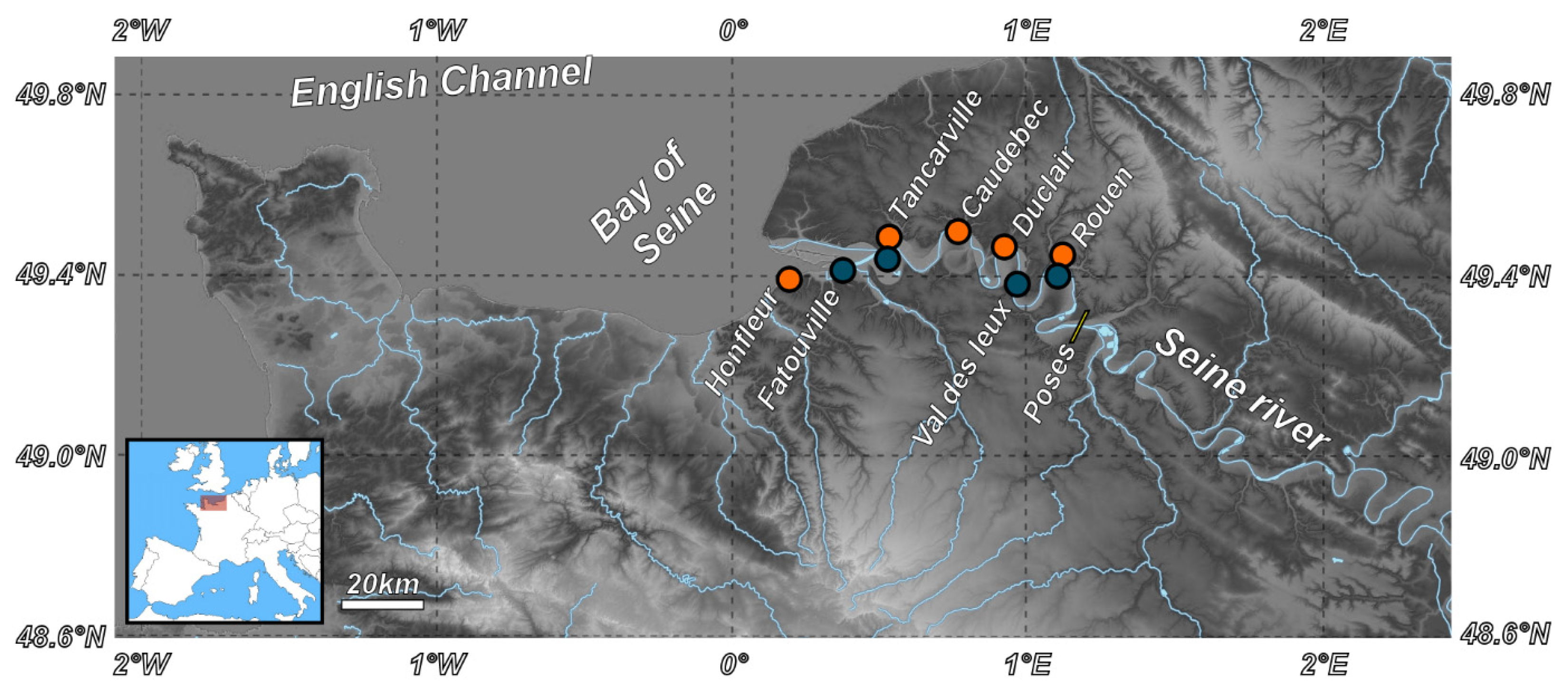
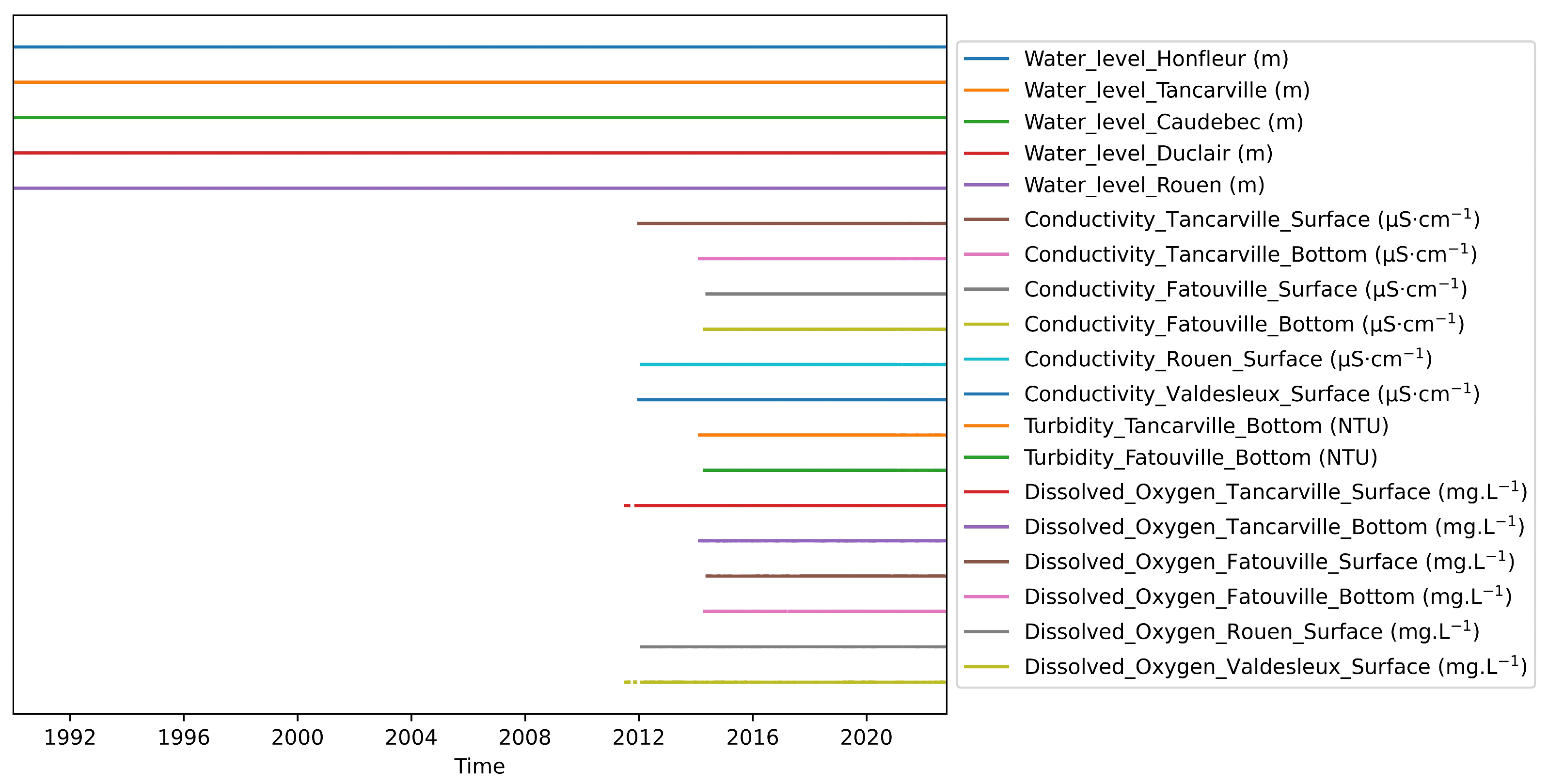
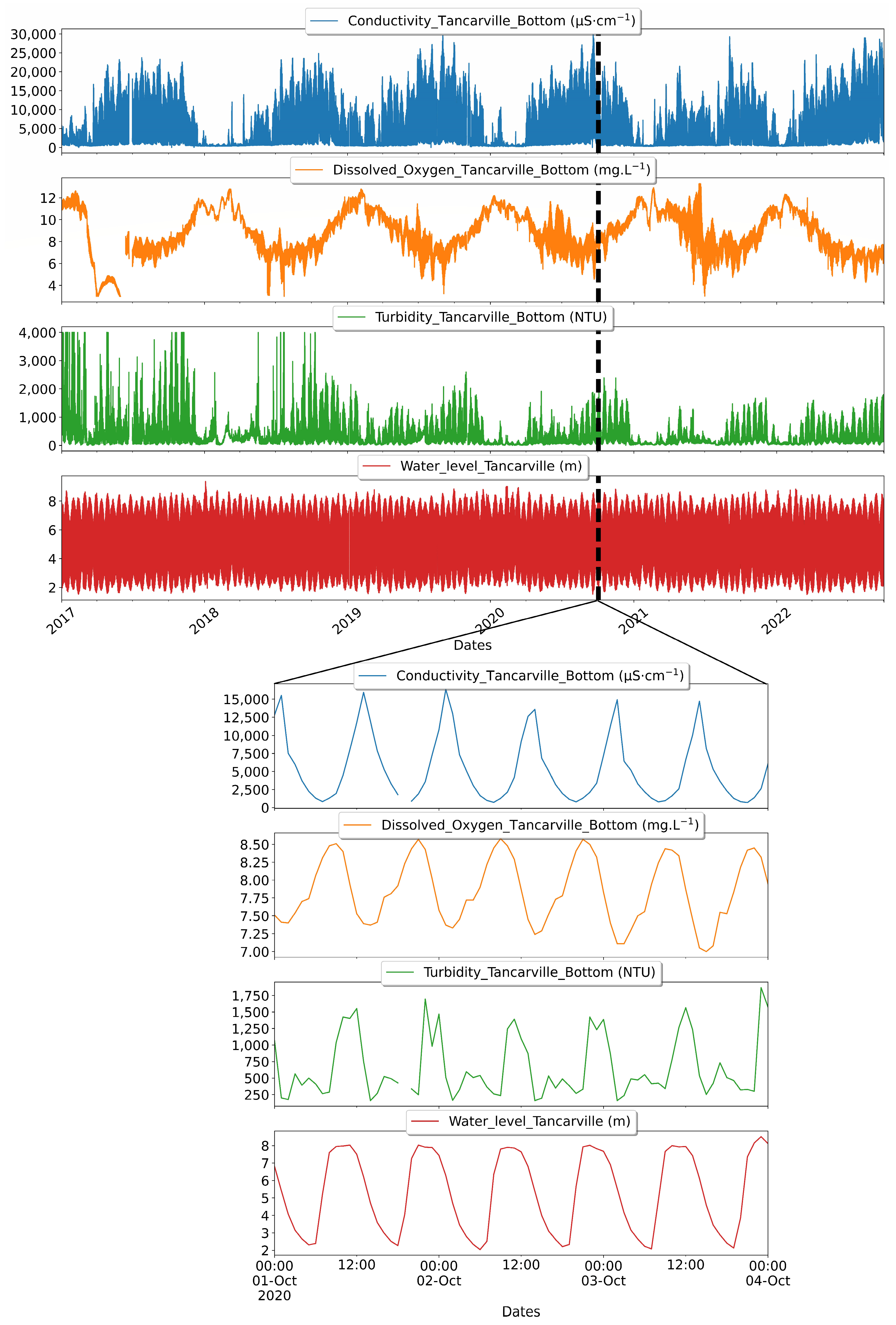
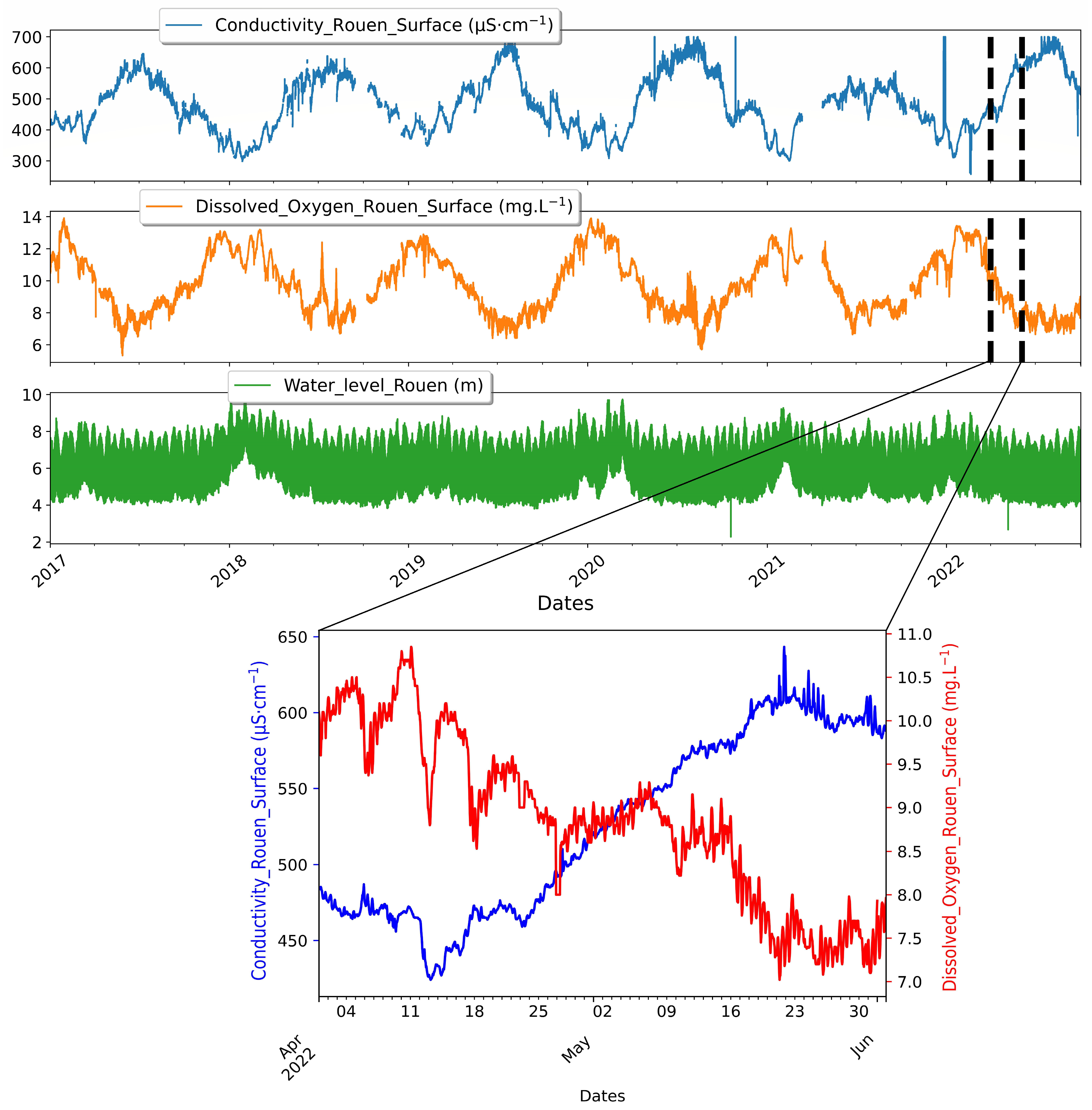
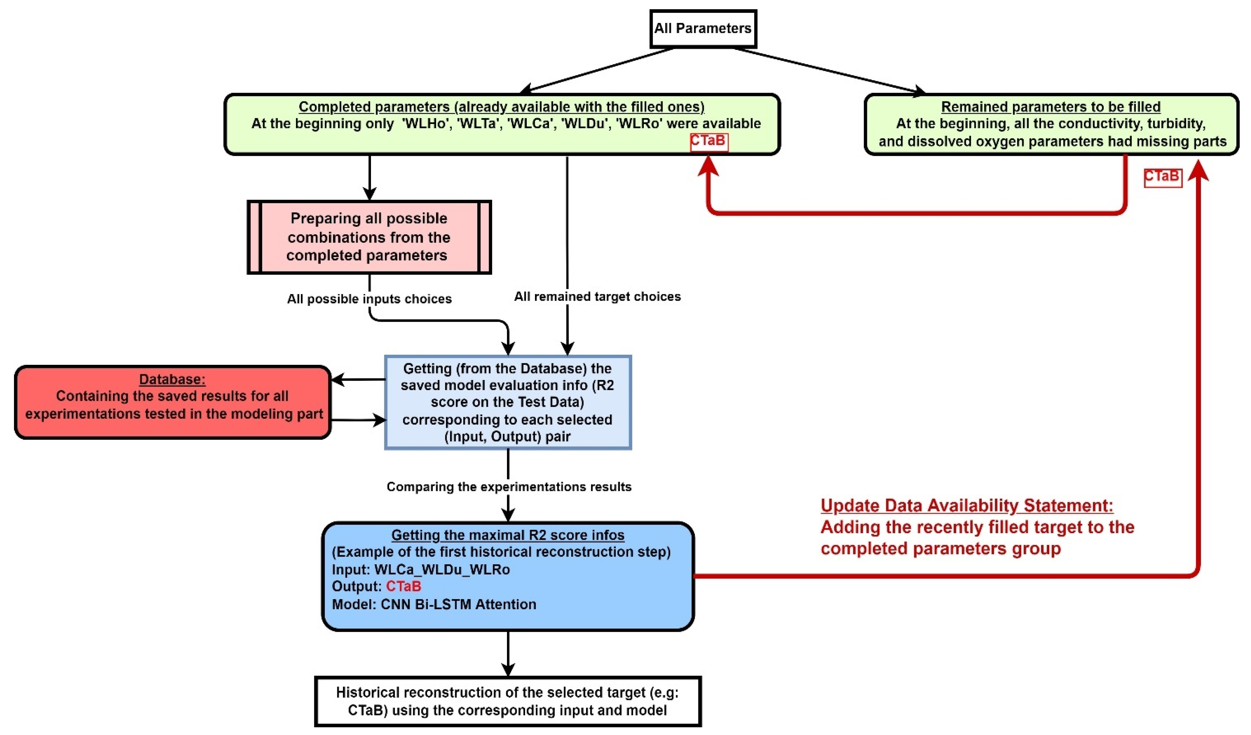
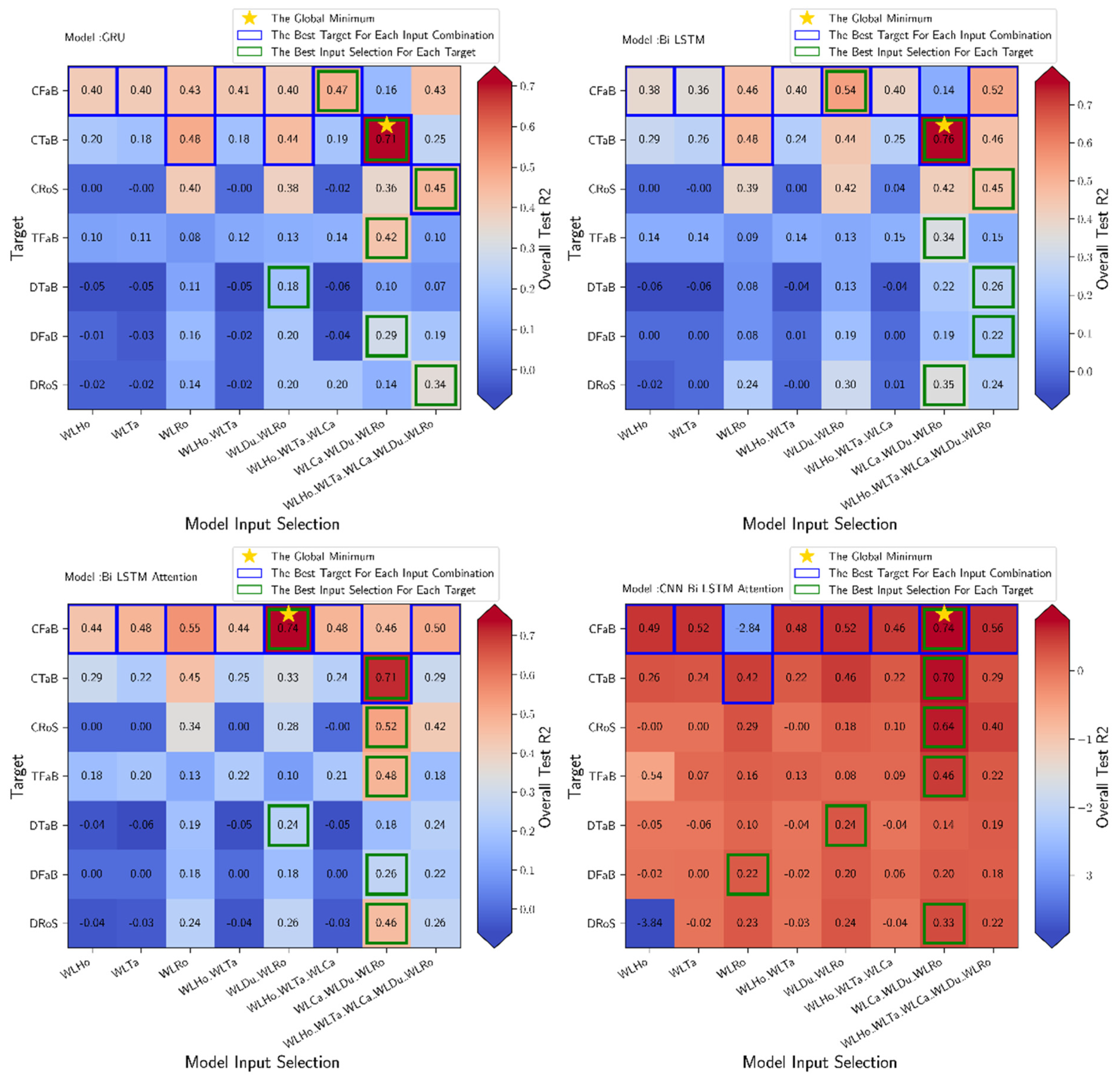
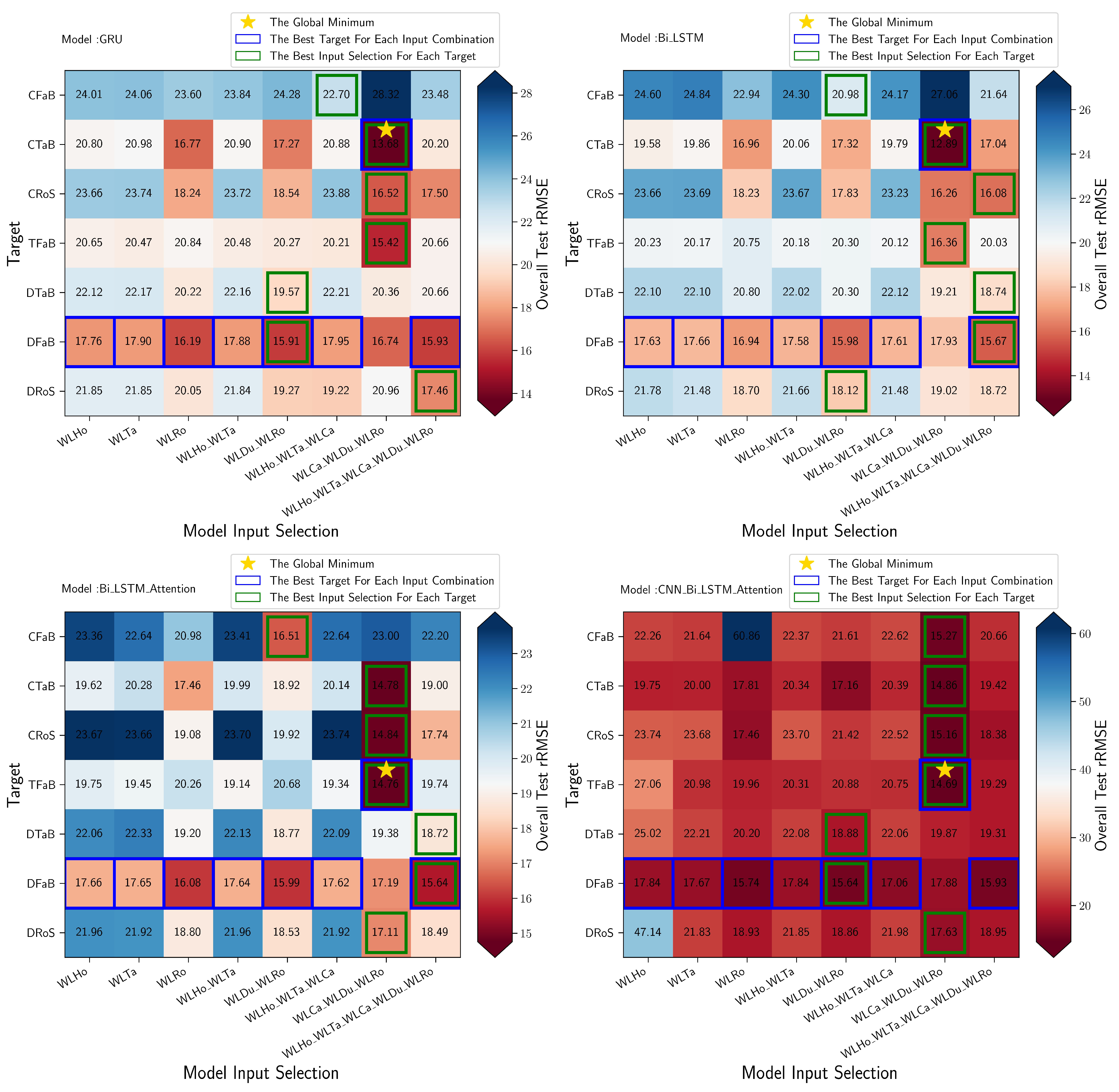
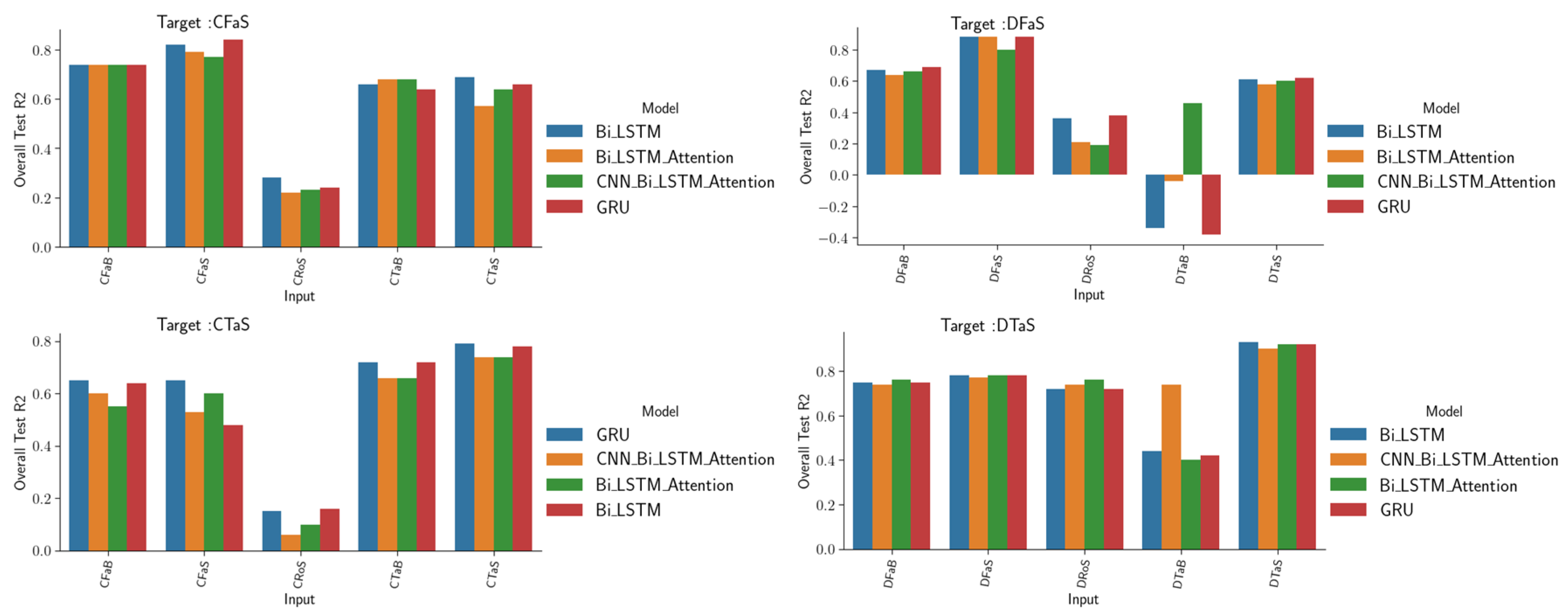
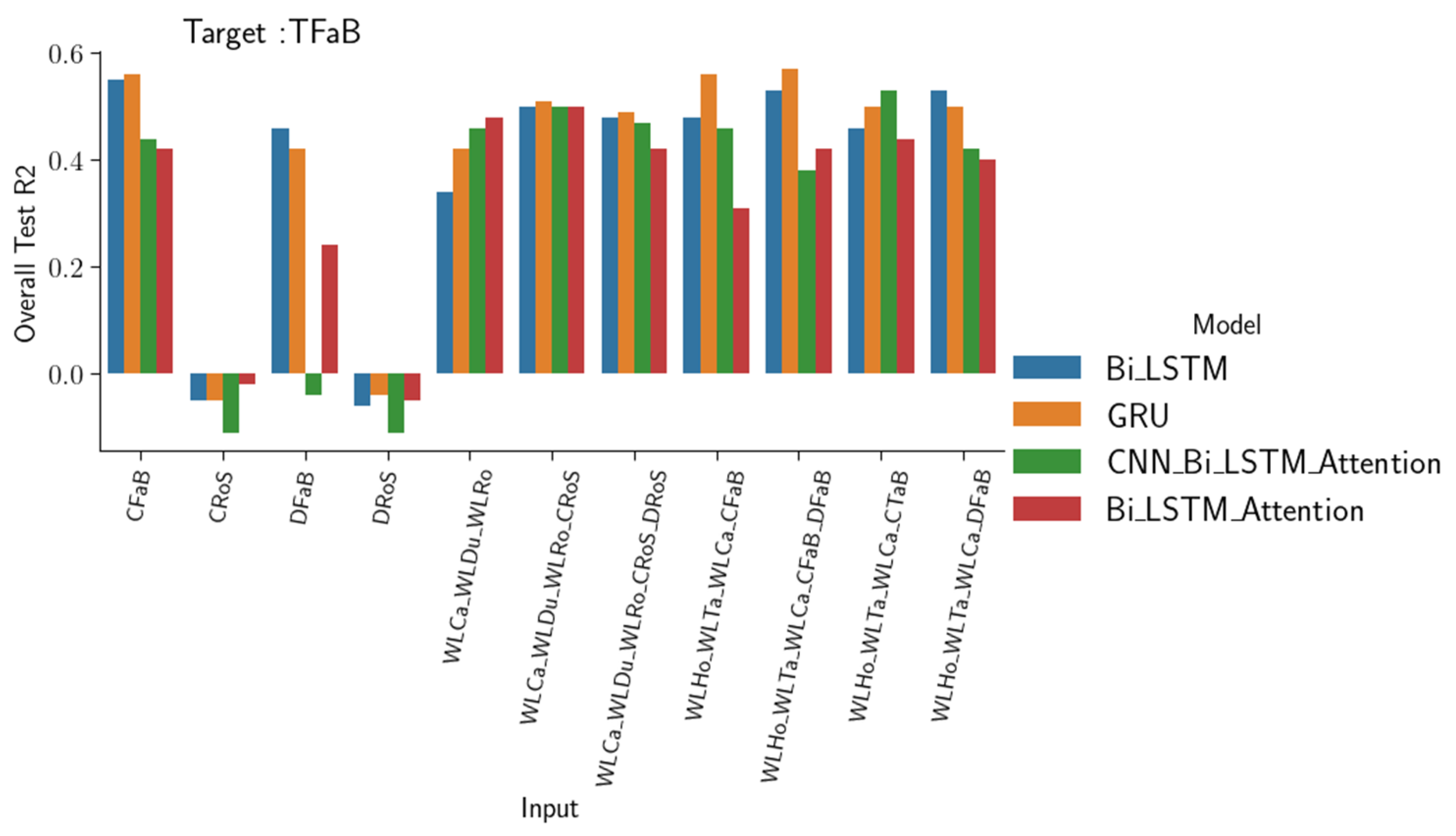
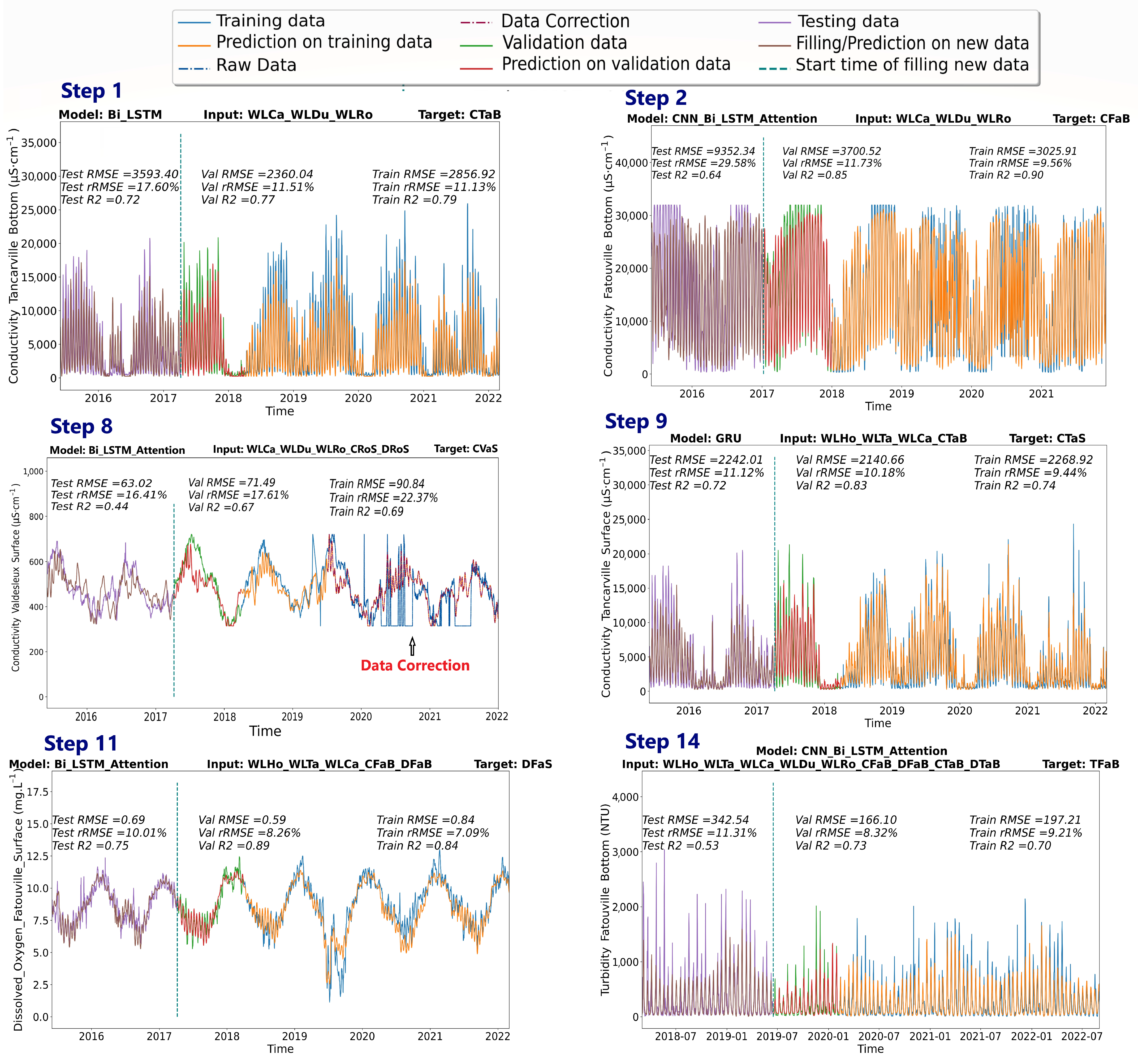
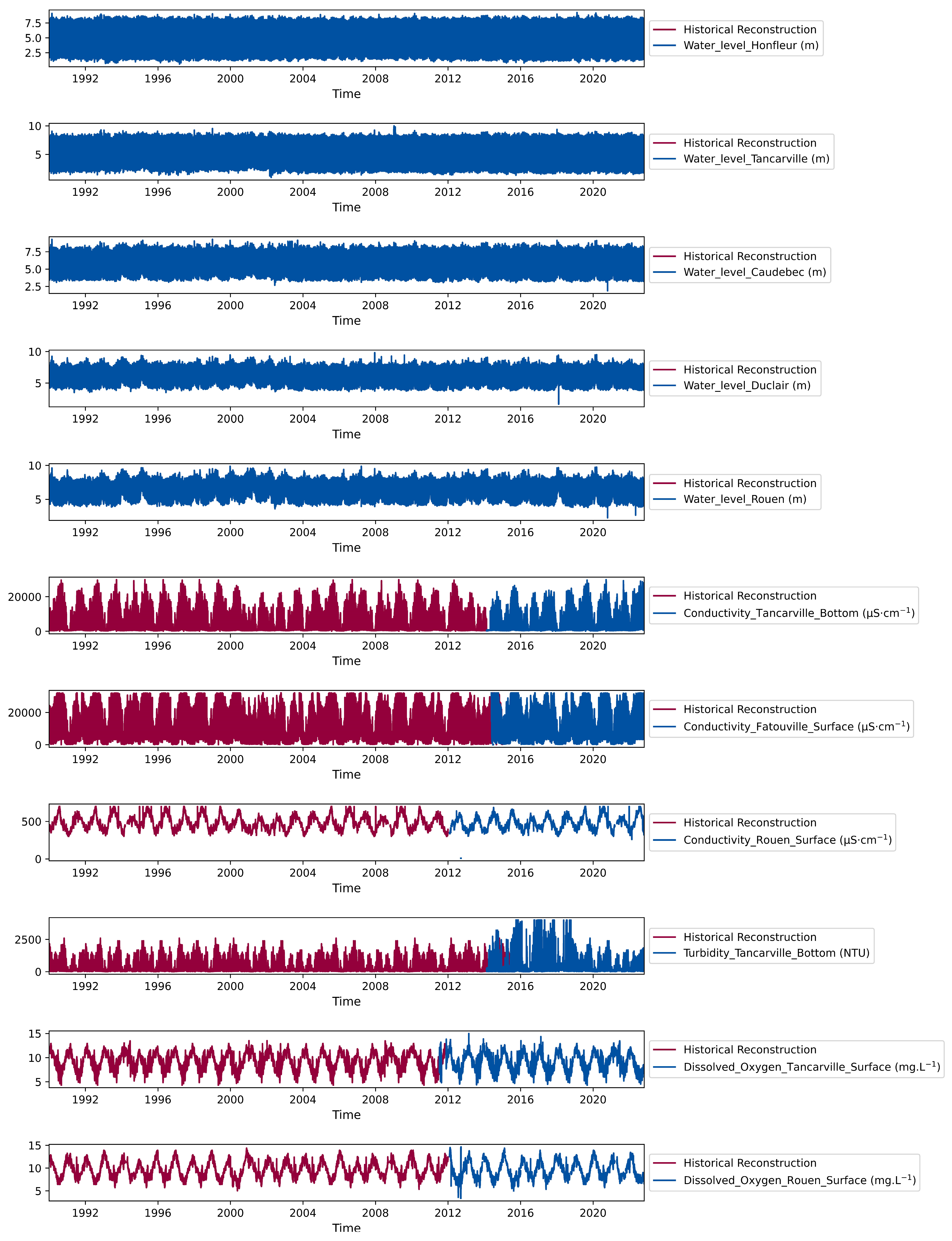
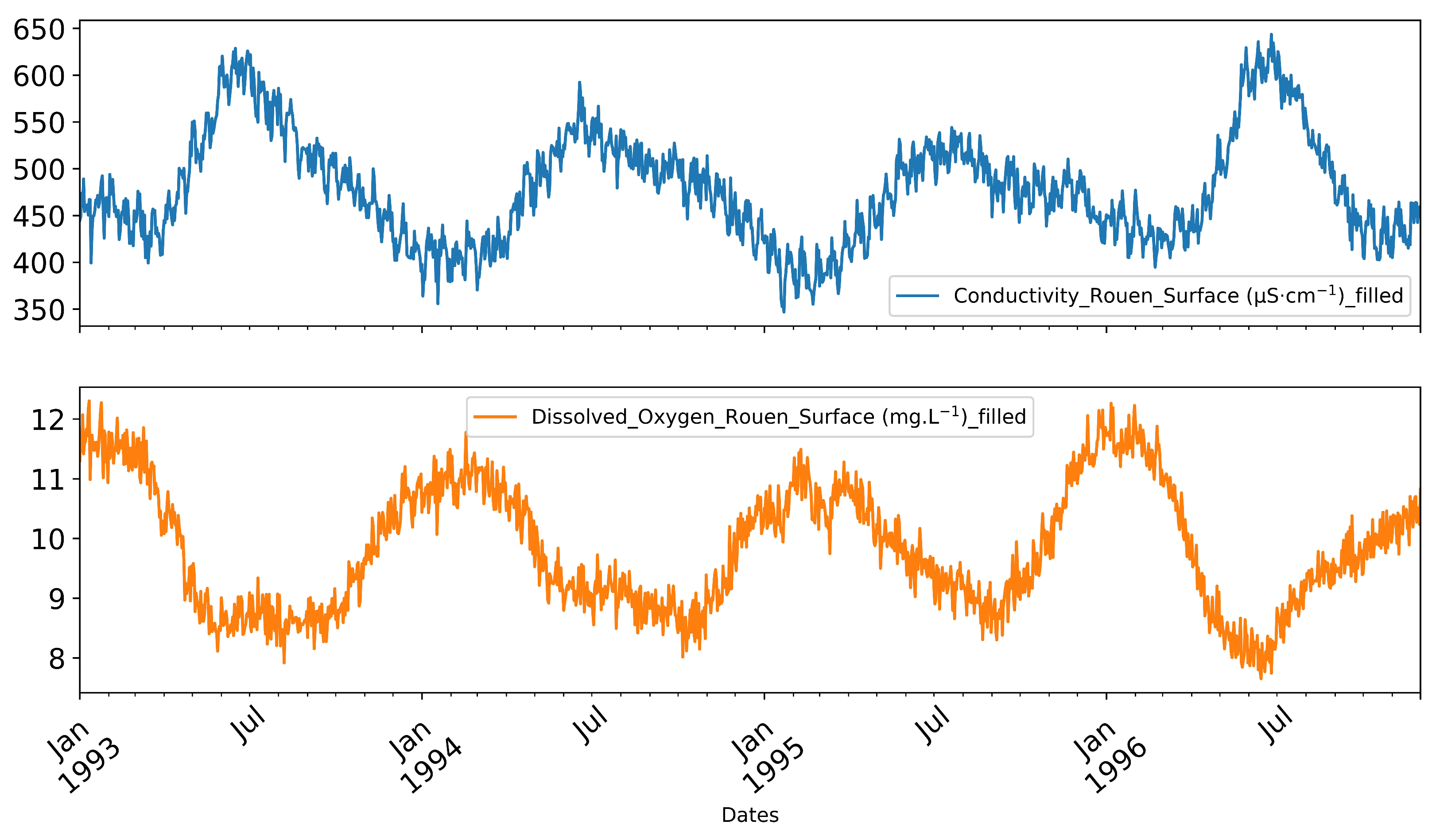
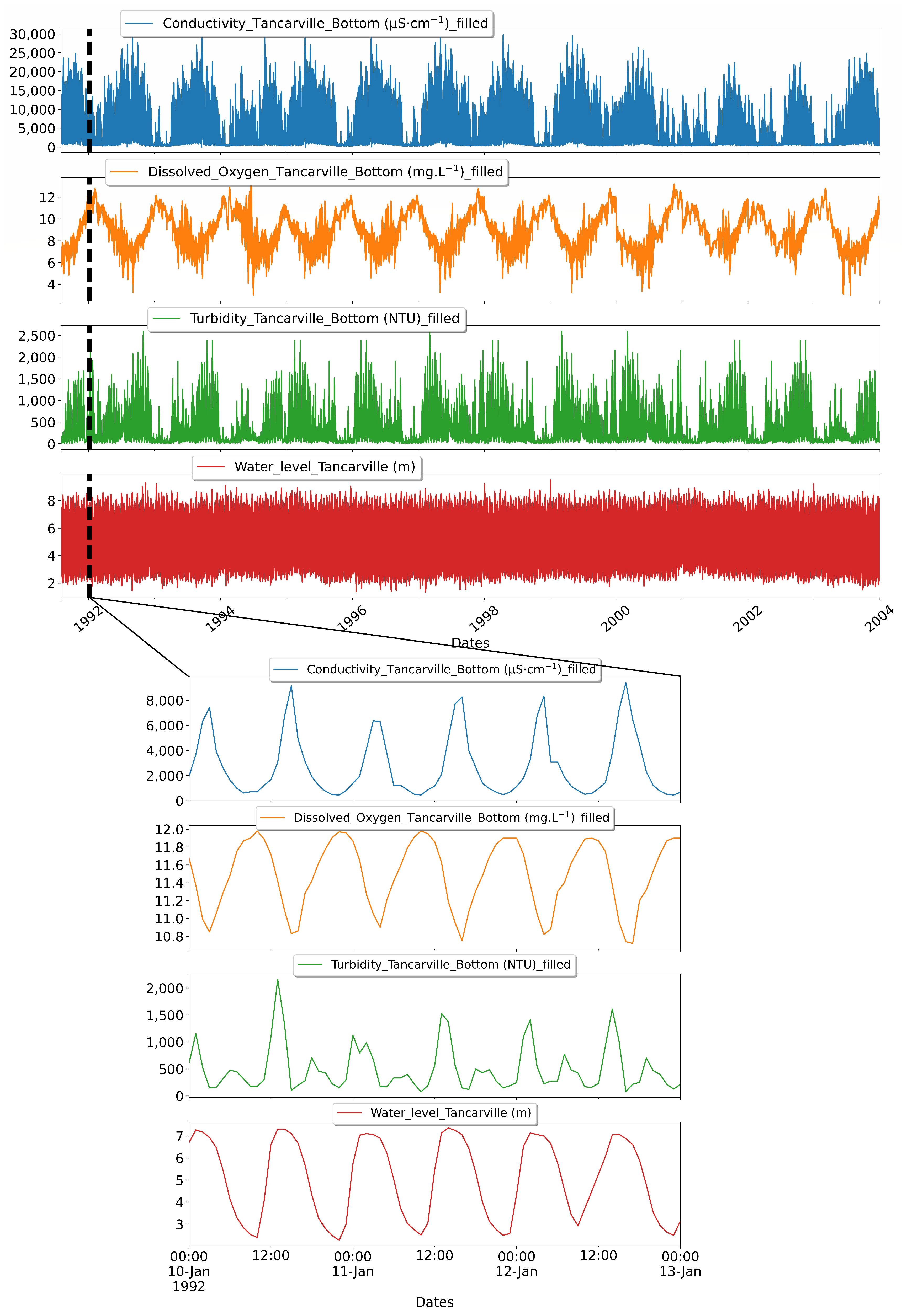
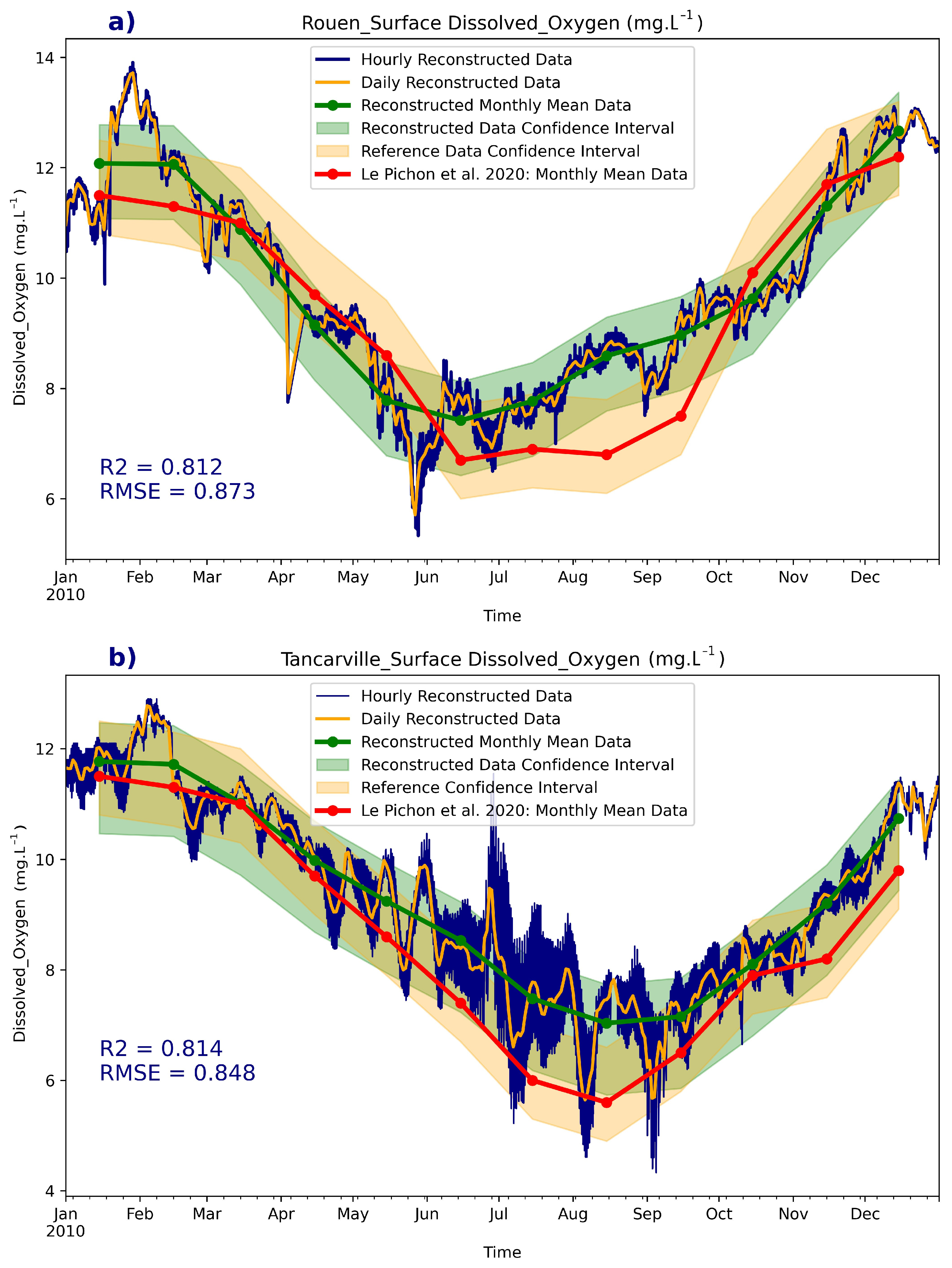
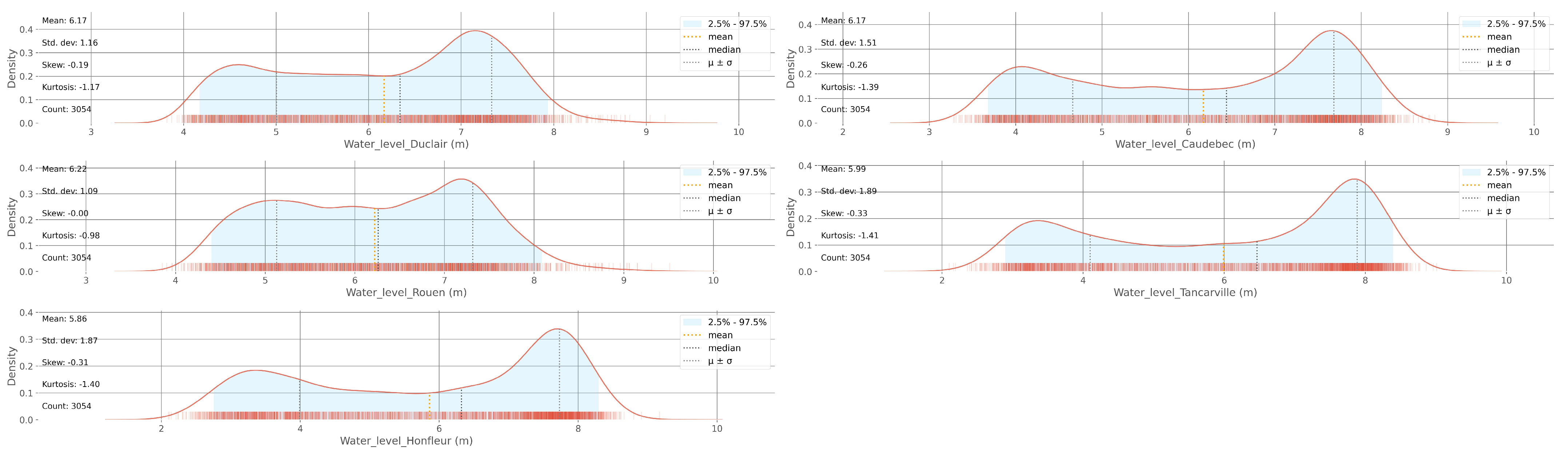
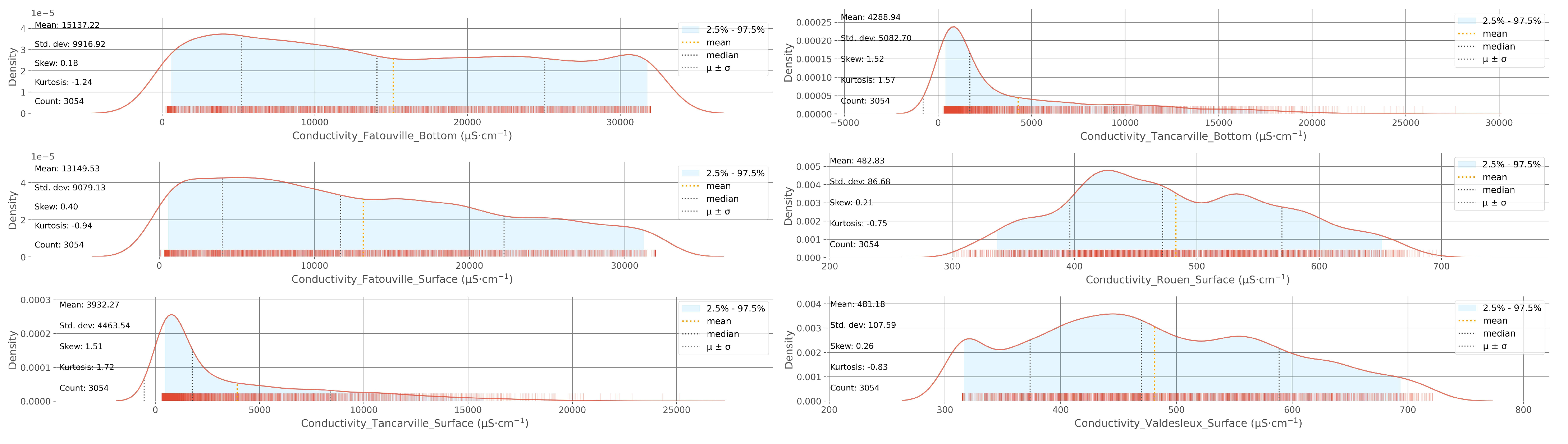
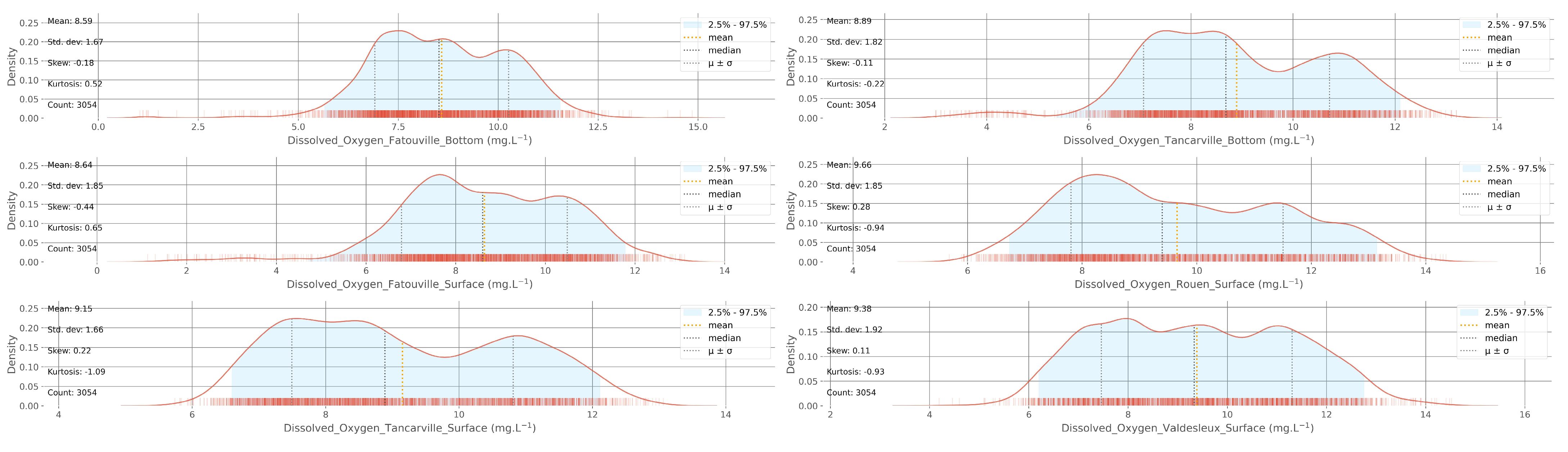
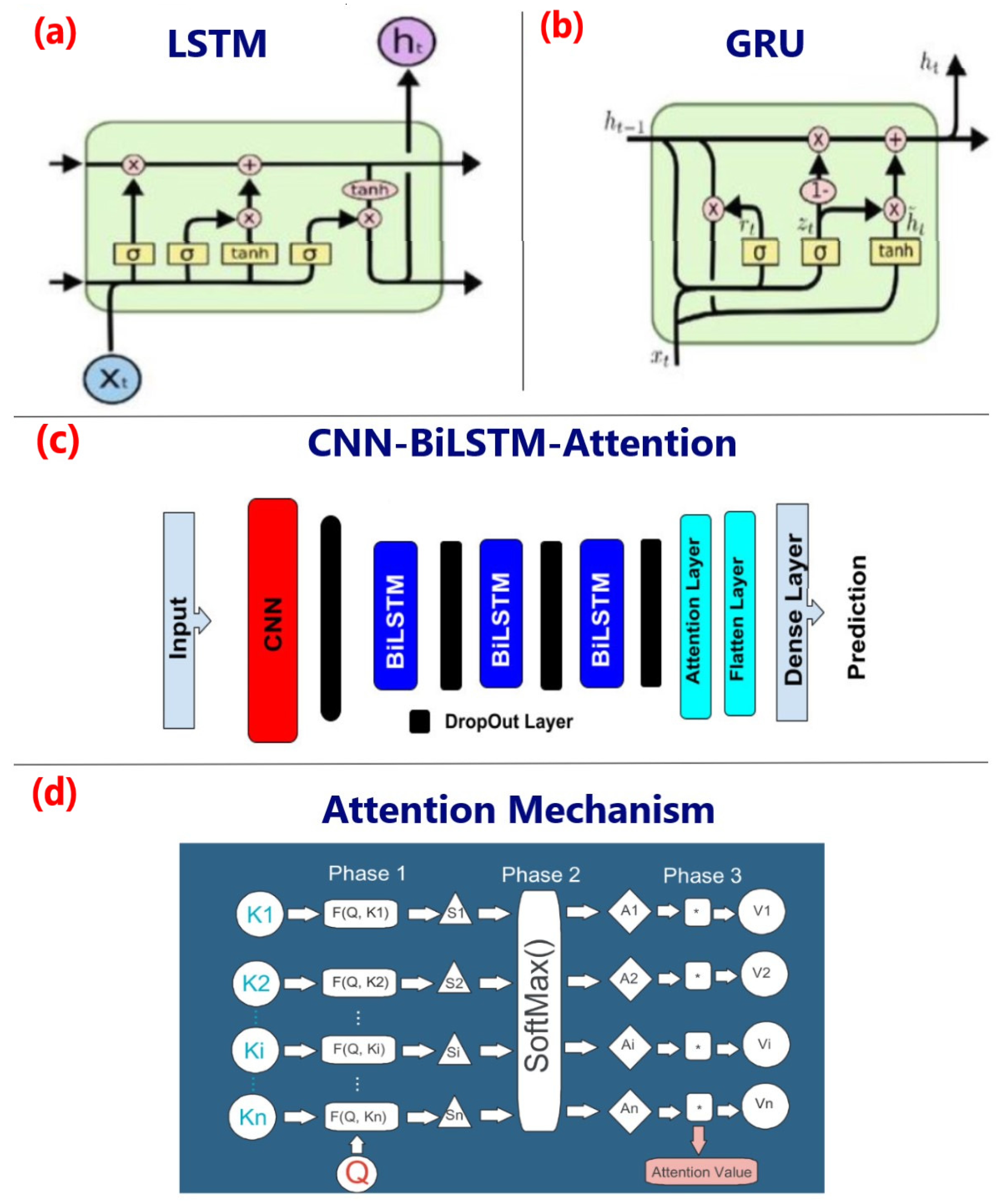
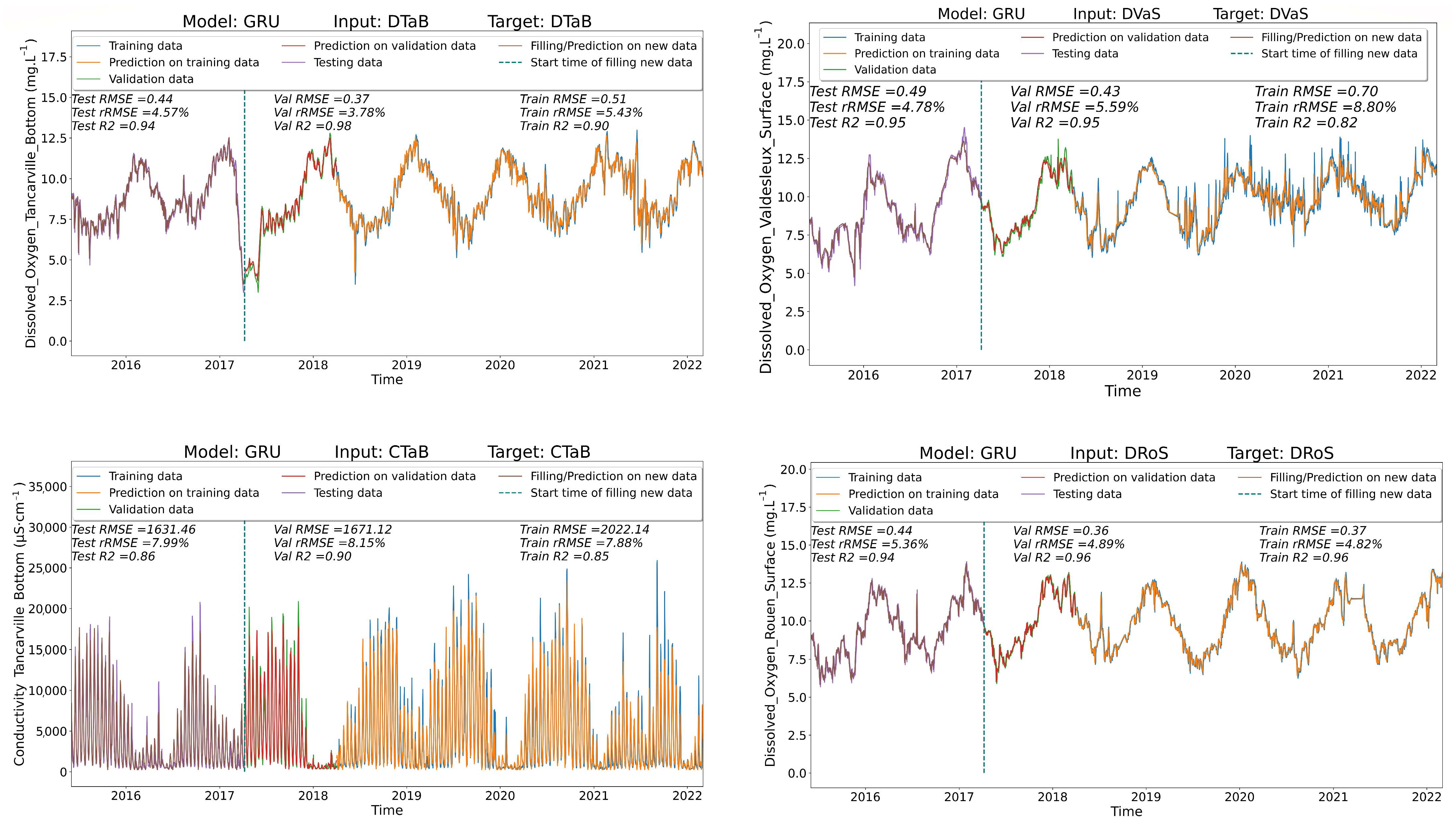
Table 1.
Abbreviations of available parameter names.
| Feature Name | Abbreviation |
|---|---|
| Water_Level_Honfleur (m) Water_Level_Tancarville (m) Water_Level_Caudebec (m) Water_Level_Duclair (m) Water_Level_Rouen (m) | WLHo WLTa WLCa WLDu WLRo |
| Electrical Conductivity_Tancarville_Surface (μS·cm−1) Electrical Conductivity_Tancarville_Bottom (μS·cm−1) Electrical Conductivity_Fatouville_Surface (μS·cm−1) Electrical Conductivity_Fatouville_Bottom (μS·cm−1) Electrical Conductivity_Rouen_Surface (μS·cm−1) Electrical Conductivity_Valdesleux_Surface (μS·cm−1) | CTaS CTaB CFaS CFaB CRoS CVaS |
| Turbidity_Tancarville_Bottom (NTU) Turbidity_Fatouville_Bottom (NTU) | TTaB TFaB |
| Dissolved_Oxygen_Tancarville_Surface (mg·L−1) Dissolved_Oxygen_Tancarville_Bottom (mg·L−1) Dissolved_Oxygen_Fatouville_Surface (mg·L−1) Dissolved_Oxygen_Fatouville_Bottom (mg·L−1) Dissolved_Oxygen_Rouen_Surface (mg·L−1) Dissolved_Oxygen_Valdesleux_Surface (mg·L−1) | DTaS DTaB DFaS DFaB DRoS DVaS |
Table 2.
Suggested range of hyperparameters fed into the Optuna hyperparameter tuning process.
| Hyper-Parameters | Range |
|---|---|
| BiLSTM/GRU Number of layers | From 1 to 4 |
| BiLSTM/GRU Number of Unit | From 10 to 500 |
| Batch-size | {32, 64, 128, 256} |
| Learning rate | From 0.001 to 0.1 |
| Drop-out | {0.1, 0.2, 0.3} |
| CNN Filter size | {4, 9, 16, 25, 36, 49, 64, 81} |
| CNN Activation Function | ‘Sigmoid’, ‘Relu’ |
| Look-Back (Input Sequence size) | From 1 day to 12 months |
Table 3.
Historical reconstruction steps with the appropriate input and model selection for each step.
Table 3.
Historical reconstruction steps with the appropriate input and model selection for each step.
| Steps | Target to Be Filled at the Specific Step | Selected Input | Selected Model |
|---|---|---|---|
| 1 | CTaB | WLCa_WLDu_WLRo | Bi_LSTM |
| 2 | CFaB | WLCa_WLDu_WLRo | CNN_Bi_LSTM_Attention |
| 3 | CFaS | CFaB | CNN_Bi_LSTM_Attention |
| 4 | CRoS | WLHo_WLTa_WLCa_CFaB | CNN_Bi_LSTM_Attention |
| 5 | DRoS | CRoS | Bi_LSTM |
| 6 | DTaS | WLCa_WLDu_WLRo_CRoS_DRoS | Bi_LSTM |
| 7 | CVaS | WLCa_WLDu_WLRo_CRoS_DRoS | Bi_LSTM_Attention |
| 8 | DVaS | DRoS | GRU |
| 9 | CTaS | WLHo_WLTa_WLCa_CTaB | GRU |
| 10 | DFaB | WLCa_WLDu_WLRo_DTaS | GRU |
| 11 | DFaS | WLHo_WLTa_WLCa_CFaB_DFaB | Bi_LSTM_Attention |
| 12 | DTaB | WLHo_WLTa_WLCa_CFaB_DFaB | CNN_Bi_LSTM_Attention |
| 13 | TFaB | WLHo_WLTa_WLCa_CFaB_DFaB_CTaB_DTaB | CNN_Bi_LSTM_Attention |
| 14 | TTaB | WLHo_WLTa_WLCa_TFaB | CNN_Bi_LSTM_Attention |
Disclaimer/Publisher’s Note: The statements, opinions and data contained in all publications are solely those of the individual author(s) and contributor(s) and not of MDPI and/or the editor(s). MDPI and/or the editor(s) disclaim responsibility for any injury to people or property resulting from any ideas, methods, instructions or products referred to in the content. |
© 2023 by the authors. Licensee MDPI, Basel, Switzerland. This article is an open access article distributed under the terms and conditions of the Creative Commons Attribution (CC BY) license (https://creativecommons.org/licenses/by/4.0/).
Share and Cite
MDPI and ACS Style
Janbain, I.; Jardani, A.; Deloffre, J.; Massei, N. Deep Learning Approaches for Numerical Modeling and Historical Reconstruction of Water Quality Parameters in Lower Seine. Water 2023, 15, 1773. https://doi.org/10.3390/w15091773
AMA Style
Janbain I, Jardani A, Deloffre J, Massei N. Deep Learning Approaches for Numerical Modeling and Historical Reconstruction of Water Quality Parameters in Lower Seine. Water. 2023; 15(9):1773. https://doi.org/10.3390/w15091773
Chicago/Turabian StyleJanbain, Imad, Abderrahim Jardani, Julien Deloffre, and Nicolas Massei. 2023. "Deep Learning Approaches for Numerical Modeling and Historical Reconstruction of Water Quality Parameters in Lower Seine" Water 15, no. 9: 1773. https://doi.org/10.3390/w15091773
Note that from the first issue of 2016, this journal uses article numbers instead of page numbers. See further details here.