Estimation of Real-Time Rainfall Fields Reflecting the Mountain Effect of Rainfall Explained by the WRF Rainfall Fields

Abstract

The effect of mountainous regions with high elevation on hourly timescale rainfall presents great difficulties in flood forecasting and warning in mountainous areas. In this study, the hourly rainfall–elevation relationship of the regional scale is investigated using the hourly rainfall fields of three storm events simulated by Weather Research and Forecasting (WRF) model. From this relationship, a parameterized model that can estimate the spatial rainfall field in real time using the hourly rainfall observation data of the ground observation network is proposed. The parameters of the proposed model are estimated using eight representative pixel pairs in valleys and mountains. The proposed model was applied to the Namgang Dam watershed, a representative mountainous region in the Korea, and it was found that as elevation increased in eight selected pixel pairs, rainfall intensity also increased. The increase in rainfall due to the mountain effect was clearly observed with more rainfall in high mountainous areas, and the rainfall distribution was more realistically represented using an algorithm that tracked elevation along the terrain. The proposed model was validated using leave-one-out cross-validation with seven rainfall observation sites in mountainous areas, and it demonstrated clear advantages in estimating a spatial rainfall field that reflects the mountain effect. These results are expected to be helpful for flood forecasting and warning, which need to be calculated quickly, in mountainous areas. Considering the importance of orographic effects on rainfall spatial distribution in mountainous areas, more storm events and physical analysis of environmental factors (wind direction, thermal cycles, and mountain slope angle) should be continuously studied.

1. Introduction

The complex topography of the Korea, with many mountainous areas, has a significant impact on the spatial pattern of rainfall. Previous studies have highlighted the importance of orographic effects on the spatial distribution of rainfall in mountainous areas [1,2,3,4,5,6,7,8]. The mountain effect, also known as the orographic effect, may cause rainfall intensification, acting as a precursor of convective storm formation [9,10]. It is expected that climate change caused by global warming will intensify the spatio-temporal variability of rainfall and extreme phenomena [11], and this mountain effect can be strengthened. However, most previous studies have focused on rainfall over longer timescales, such as daily, monthly, and yearly timescales. The effect of mountains on the spatial distribution of rainfall is more pronounced in the long timescale, while the relationship between rainfall and elevation becomes more complex in the short timescale [12]. Nonetheless, for the flood forecasting and warning, the influence of elevation at these shorter timescales is critical, especially in mountainous areas with a limited number of ground rainfall observation sites. External drift kriging and co-kriging methods using the statistical relationship between ground observed rainfall data and elevation have been used to obtain the rainfall field in the void space of the ground observation network [13,14,15]. However, on a short timescale, there are often cases where rainfall occurs only in some areas, and it is often impractical to estimate an appropriate variogram in real time, making it difficult to apply models based on kriging.

The scarcity of studies investigating the relationship between rainfall and elevation on short timescales can be attributed to the limited spatial density of ground observation networks in mountainous areas. Typically, the maximum spatial scale for investigating the rainfall–elevation relationship at the hourly timescale is considered to be the meso-γ-scale, which is approximately around 5 km. [16,17]. However, in most regions, including the Korea, it is challenging to find ground observation networks with such high spatial density. Consequently, the current ground rainfall observation network may underestimate or overestimate the spatial rainfall of the watershed, leading to distortions not only in the estimation of flood volume but also in the assessment of the watershed’s hydrologic cycle.

Over the last 30 years, there has been a significant improvement in the quality of rainfall simulations produced by numerical weather forecasting models at global, regional, and local scales. For example, Ohara et al. [18] successfully reconstructed past typhoon precipitation using MM5 (Fifth-Generation Penn State/NCAR Mesoscale Model) [19], while Wu et al. [20] simulated typhoon rainfall using various weather prediction numerical models such as the WRF (Weather Research and Forecasting) model, HWRF (Hurricane Weather Research and Forecasting) model, MM5, and CReSS (Cloud Resolving Storm Simulator) and identified the optimal combination of these ensembles. Karki et al. [21] used WRF to simulate extreme heavy rain events in Nepal and evaluated the location and intensity of rainfall events through sensitivity analysis of the physical options in WRF. Similarly, Patel et al. [22] utilized WRF to predict extreme flooding in western coastal cities of India, and Caumont et al. [23] simulated extreme storm events in France using a weather prediction numerical model. While numerical weather forecasting models excel in consistently simulating the dynamics of the atmosphere and addressing orographic precipitation generation mechanisms more accurately [9], their long computing time makes them unsuitable for forecasting and warning purposes.

This study aims to estimate a real-time rainfall field in the Namgang Dam watershed by using rainfall data observed at ground observation sites. The purpose is to improve the reliability of flood estimation for flood forecasting and warning in the mountainous region. The focus of the research is on extreme rainfall and its spatio-temporal distribution, with a perspective on hydrology and disaster prevention. This approach may differ from research that takes into account various weather factors such as atmospheric pressure and wind speed.

The research schematic diagram depicted in Figure 1 illustrates the methodology used in this study. The rainfall time series from 2001 to 2020 in the target area were analyzed, and storm events were selected and simulated using the WRF model. The spatial rainfall field is reconstructed from the WRF simulation results through bias correction using ground observation data. The INCA (Integrated Nowcasting through Comprehensive Analysis) algorithm, developed by ZAMG (Austrian Central Institute for Meteorology and Geodynamics), is applied to quantify the relationship between rainfall and elevation in the Namgang Dam watershed using the reconstructed rainfall field and ground observation data. Additionally, a rainfall field estimation model, which is associated with elevation, is proposed based on this relationship. Finally, the practical applicability of the proposed model is assessed using leave-one-out cross-validation (LOOCV) for seven ground observation sites in the mountainous region of the Namgang Dam watershed.

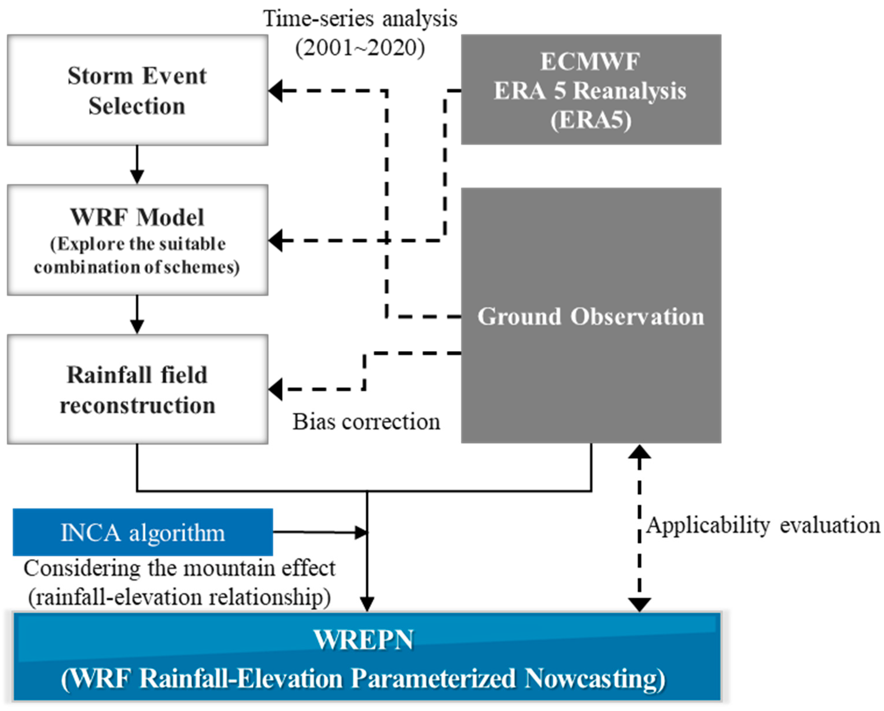
2. Materials and Methods

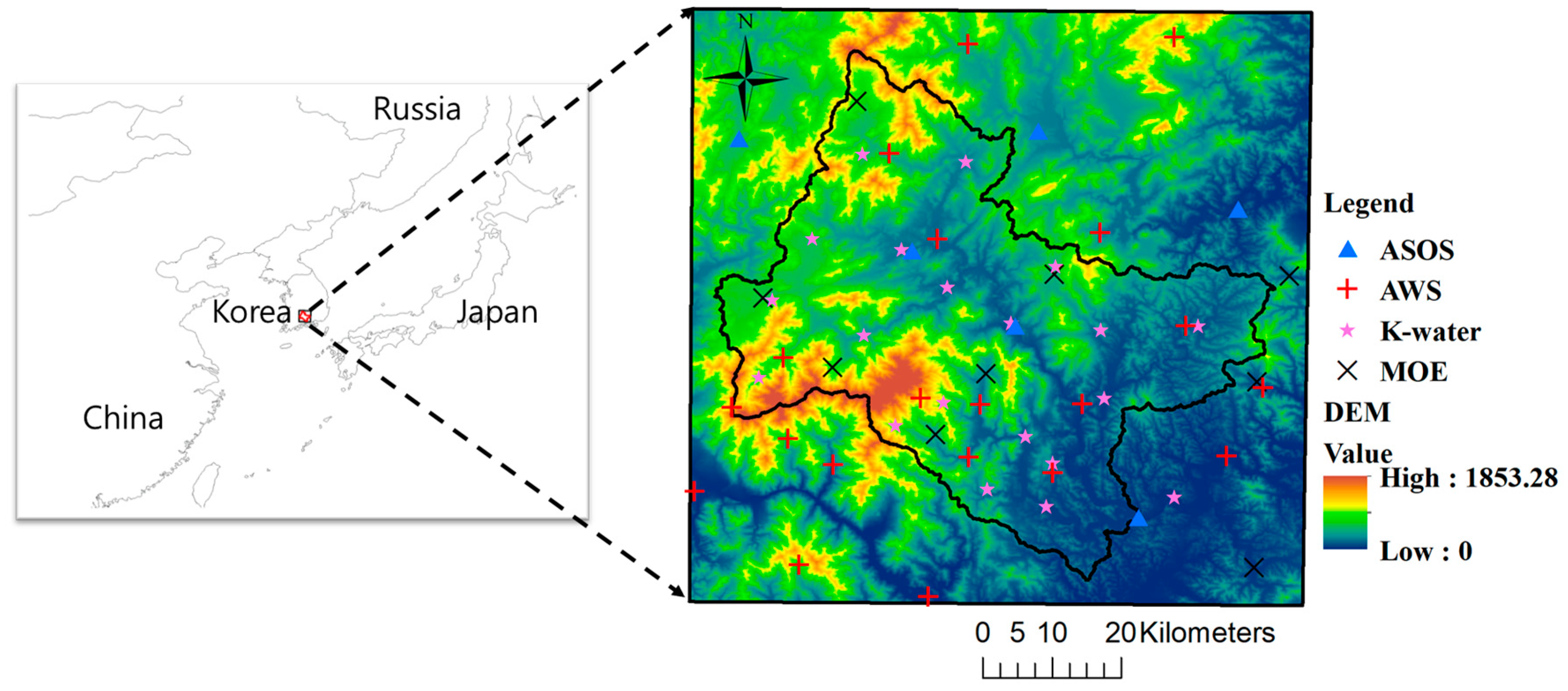
2.1. Target Area and Storm Events

The Namgang Dam watershed is a representative mountainous region in the Korea, with a highest elevation of 1853 m and a lowest elevation of 35 m based on a digital elevation model with a spatial resolution of 90 m. For this study, the target area shown in Figure 2 was selected, which includes 55 ground rainfall observation sites. The elevation of the lowest operating site is 4.5 m, while the highest site has an elevation of 1087.9 m.

Storm events that occurred in 2003, 2007, and 2020 were selected for WRF modeling. The storm event that occurred in 2003 was associated with Typhoon Maemi, which recorded the highest accumulated rainfall (about 250 mm) in the Namgang Dam watershed among typhoons that have affected the Korea in the past 30 years. The storm event that occurred in 2007 was selected from among the storm events that showed an abnormally large runoff rate in Namgang Dam watershed. This storm event was also related to Typhoon Nari, and the official record of the inflow of flooding from Namgang Dam showed a runoff rate of 1.02 at this time. The storm events that occurred in 2020 were chosen as relatively recent extreme storm events. This storm event showed a pattern of torrential rainfall that was not related to a typhoon, and it is a storm event that occurred during an unprecedentedly long rainy season.

2.2. WRF

WRF (Weather Research and Forecasting) is a community weather forecasting numerical model developed in cooperation with more than 150 organizations around the world, centered on the US National Center for Atmospheric Research (NCAR). As of 10 May 2021, version 4.3 is provided, and this version was used in this study.

To simulate rainfall using WRF, it is necessary to explore the scheme of physics options suitable for the target area and storm event [22]. Among the physical options generally used in WRF, MP (microphysics), CU (cumulus parameterization), and PL (planetary boundary layer) are known as major physical options that affect rainfall [24,25]. In addition to these physical options, RA_L (longwave radiation) and RA_S (shortwave radiation) have been added to the latest version of WRF. In this study, the selected storm events were reproduced by numerical experiments with various combinations of schemes available in the five physics options. Various experiments were performed, consisting of the seven different MP (Goddard 4-ice, Ferrier Eta, Stony-Brook University, Thompson, WRF Double Moment 6-class, WRF Single-Moment 5-class, and WRF Single-Moment 6-class scheme), four CP (Betts–Miller–Janjic, Kain–Fritsch, New Tiedtke, and Tiedtke scheme), two different PL (Mellor–Yamada–Janjic, Yonsei University scheme), two different RA_L (RRTM, RRTMG scheme), and two different RA_S (Dudhia, RRTMG scheme) schemes.

The spatial domain driving the WRF consists of three-level domains. The final domain was configured with a spatial resolution of 3 km (see Figure 3). However, the simulated rainfall fields were analyzed by limiting them to the area corresponding to Figure 2 inside the domain D-3.

Even if a storm event is reconstructed using the combination of physics options–scheme that is most appropriate for each storm event, the observed rainfall from ground observation networks cannot be fully reproduced. In this study, conditional merging (CM) [26] was used to perform bias correction for the simulated rainfall field through the following procedure:

(1) Obtain the rainfall field $R_s\left(x\right)$ simulated by WRF.

(2) Generate the interpolated spatial rainfall field $R_{ko}\left(x\right)$ using co-kriging from ground observation network data.

(3) Generate the rainfall field $R_{ks}\left(x\right)$ interpolated by co-kriging by extracting data of pixels where the ground observation network is located from $R_s\left(x\right)$.

(4) Calculate the difference of the simulated and observed rainfall fields as ${∆R}_s\left(x\right)=R_s\left(x\right)-R_{ks}\left(x\right)$.

(5) Obtain the bias-corrected rainfall field $R_{cs}\left(x\right)=R_{ko}\left(x\right)+∆R_s\left(x\right)$, where $R_{cs}\left(x\right)$ represents the bias-corrected rainfall field, $R_{ko}\left(x\right)$ represents the interplated spatial rainfall field.

2.3. Estimation Model of Rainfall Field Associated with Elevation

The algorithm introduced in this study has been successfully applied to the Austrian INCA nowcasting system [27,28], and relatively recently applied to account for the mountain effect of rainfall near Beijing, China [29]. The rainfall field estimation algorithm considering the elevation effect on rainfall is designed depending on the magnitude of the rainfall intensity. The equation of the proposed algorithm is as follows.

$$P_m=\left\{\begin{array}{c}{P}_v(a-b·P_v)\\ P_v+(a-1-b·P_c)P_c\end{array}\genfrac{}{}{0pt}{}{, for P_v\le P_c}{, for P_v>P_c}\right.$$

(1)

where $P_m$ and $P_v$ are mountain and valley rainfall, respectively, and $P_c=(a-1)/\left(2b\right)$. Parameters $a$ and $b$ were estimated to minimize the difference between observed $P_m$ (simulated by the WRF in this study) and the calculated $P_m$ using Equation (1).

To extend the relationship in the mountain–valley station pair to the rainfall field, we first construct the station-based terrain $Z_{st}(i,j)$ interpolated with the inverse distance weighting method (IDW) using the elevation of the pixel where the station is located. Here, $(i,j)$ denotes a pixel position, $i$ denotes a longitude direction, and $j$ denotes a latitude direction. Then, using the relationship between valley and mountain rainfall in Equation (1), the relative rainfall increment field is calculated as follows.

$$G\left(i,j\right)=\frac{P_m\left(i,j\right)-P_v(i,j)}{z_r}$$

(2)

where $P_v$ is a rainfall field that interpolates rainfall data of a pixel with an observation site using IDW, and $P_m$ can be calculated by applying the parameters $a$, $P_c$, and $P_v$ to Equation (1). The $z_r$ is the average elevation difference of mountain–valley pixels used to construct the relationship of Equation (1) ($z_r$ = 528 m in this study). That is, $G$ is the rainfall increment per unit meter of mountain.

Therefore, the geographic rainfall increases due to the elevation effect $∆P$ can be obtained as follows.

$$∆P\left(i,j\right)=G(i,j)·[\widehat{Z_H}\left(i,j\right)-Z_{ST}(i,j)]$$

(3)

where $\widehat{Z_H}$ conceptually represents the actual elevation, but because the reduction in the mountain effect at a high elevation above a certain level should be reflected, the adjusted elevation is applied as follows.

$$\widehat{Z_H}=\left\{\begin{array}{c}{Z}_{MAX}-∆Z·exp\left[-\frac{Z_H-Z_{MAX}+∆Z}{∆Z}\right]\\ Z_H\end{array}\right.\genfrac{}{}{0pt}{}{\begin{array}{c},for Z_H>Z_{MAX}-∆Z\\ \end{array}}{,for Z_H\le Z_{MAX}-∆Z}$$

(4)

where $Z_H$ is the actual elevation, and $Z_{max}$ and $∆Z$ are 1500 m and 250 m, respectively.

Finally, the hourly rainfall field $P_E$ considering the mountain effect is composed as follows.

$$P_E\left(i,j\right)=P_v\left(i,j\right)+∆P\left(i,j\right), \mathrm{for} ∆P\left(i,j\right)>0$$

(5)

In this case, $P_E\left(i,j\right)=P_v\left(i,j\right)$ is applied to a pixel with $∆P\left(i,j\right)\le 0$.

3. Results and Discussion

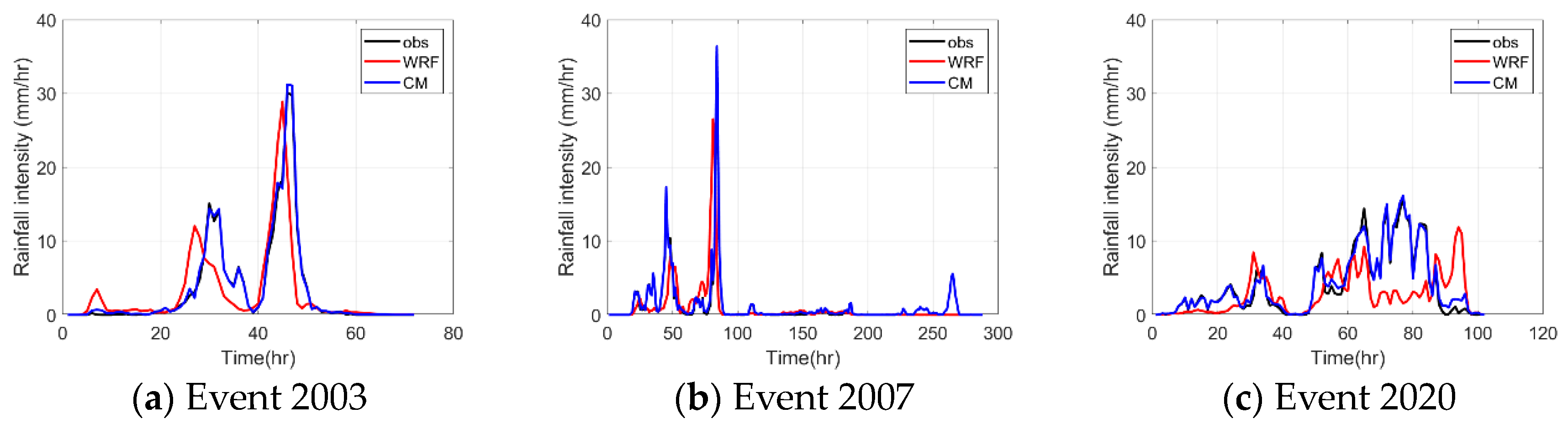
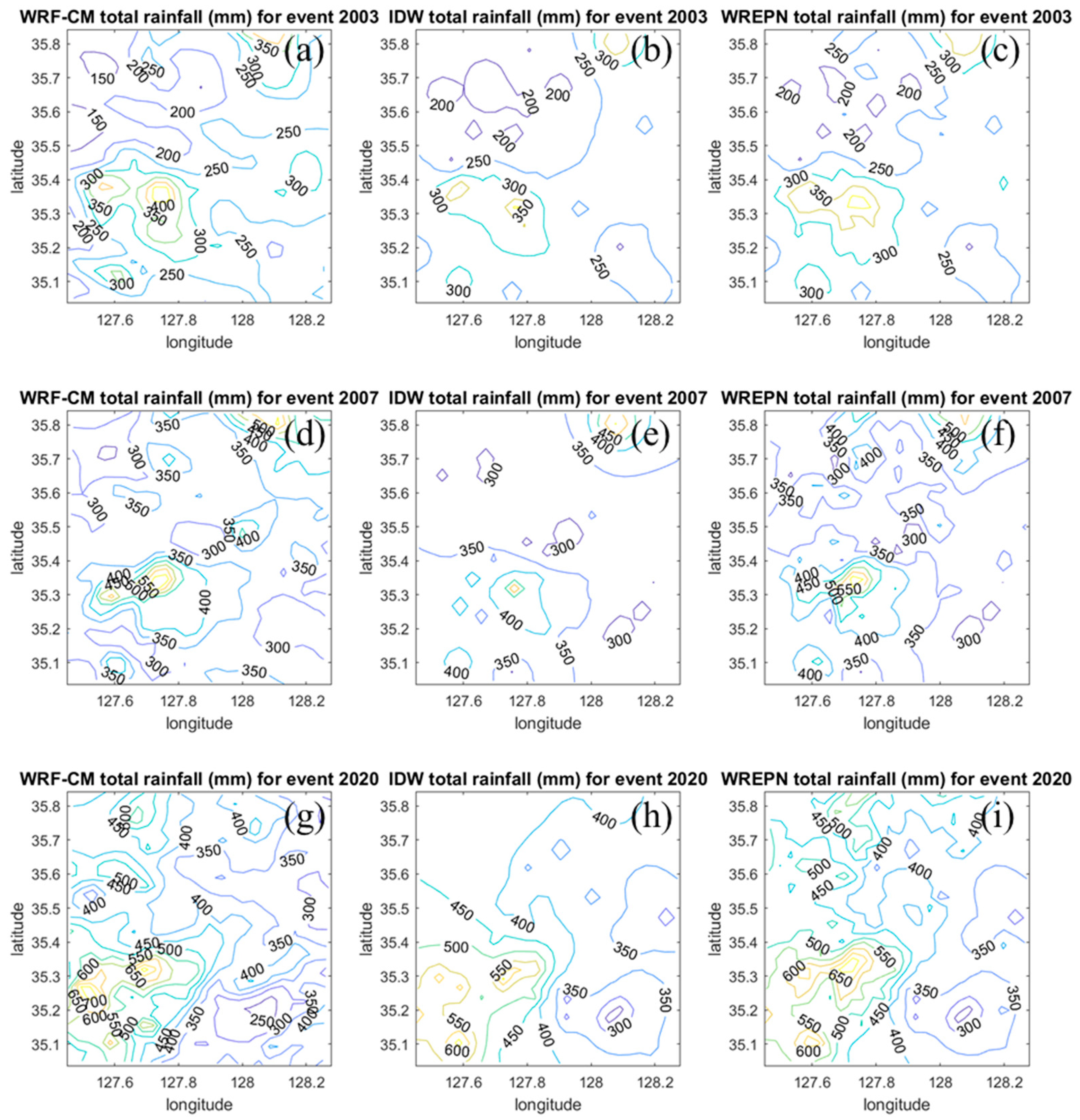
3.1. WRF Simulation Results

In order to run WRF, initial and boundary conditions are necessary, and these have a significant impact on the simulated results of WRF. For initial and boundary condition data, the following data are commonly used: (1) National Centers for Environmental Prediction (NCEP) Final Operation Model Global Tropospheric Analyses (hereinafter referred to as NCEP-FNL); (2) NCEP’s GDAS/FNL 0.25 Degree Global Tropospheric Analyses and Forecast Grids (hereinafter NCEP-GDAS/FNL); (3) ERA-Interim Project (hereinafter ERA-Interim) of the European Center for Medium-range Weather Forecasts (ECMWF); and (4) ERA 5 Reanalysis of ECMWF (ERA5). Among them, ERA5, which provides information at 1 h intervals and a resolution of 0.25°, has been judged to be particularly useful due to its high resolution and accuracy. It also showed the best agreement when compared with the ASOS (Automated Synoptic Observing System) and AWS (Automatic Weather System) data of the Korea Meteorological Administration. Therefore, in this study, initial and boundary condition data were constructed based on ERA5. However, the initial and boundary conditions generated with a spatial resolution of 0.25° are difficult to reconstruct the detailed spatial distribution expressing the extreme values, so the initial and boundary conditions were improved using additional data. In this study, the initial and boundary condition data were improved by additionally inputting NCEP ADP Global Surface Observational Weather Data, which is the surface and sea level observation data constructed in NCEP ADP Global Upper Air Observational Weather Data and the Global Telecommunications System (GTS), which includes various terrestrial and satellite observation systems operated by NCEP.

Numerical experiments were performed by configuring various combinations for each storm event to select the optimal combination of physics options–scheme. The number of combinations mentioned in Section 2.2 is a total of 224, and it is not practically appropriate to conduct numerical experiments for all of them to reconstruct a single storm event. Therefore, referring to the existing literature conducted on the Korean region (e.g., [30,31,32,33,34]), numerical experiments were performed by configuring as few as 15 combinations and as many as 37 combinations for each storm event.

Table 1. Optimal scheme combination for each storm event.

Storm Event	Event 2003	Event 2007	Event 2020
MP	WRF Single-Moment 6-class	WRF Single-Moment 6-class	Thompson scheme
CU	New Tiedtke scheme	New Tiedtke scheme	Tiedtke scheme
PB	Mellor–Yamada–Janjic scheme	Yonsei University scheme	Yonsei University scheme
RA_L	RRTMG scheme	RRTMG scheme	RRTMG scheme
RA_S	RRTMG scheme	RRTMG scheme	RRTMG scheme

shows the optimal physics option–scheme combination corresponding to each storm event.

In order to examine the spatial reproducibility of the simulated storm event, Figure 4 shows the rainfall field which was interpolated by the co-kriging method of the accumulated rainfall observed from the ground observation network (obs in Figure 4), the simulated accumulated rainfall from the WRF (WRF in Figure 4), and the cumulative rainfall field which was bias-corrected for each hour of the WRF rainfall field using CM (CM in Figure 4). WRF simulated a lot of rainfall in the middle of Jirisan Mountain (southwest of Namgang Dam watershed) for all three storm events, and it can be confirmed that this is similar to the spatial distribution of the observed rainfall field. Although there is a difference between the cumulative rainfall of WRF and the observed cumulative rainfall, it can be found that this difference is removed by performing bias correction using CM.

Figure 5 shows the temporal distribution of spatially averaged rainfall for each storm event. While WRF rainfall reconstructs the temporal distribution of the observed rainfall well for Events 2003 and 2007, it does not reconstruct this for Event 2020. Nevertheless, performing bias correction using CM enables the temporal distribution of rainfall to also closely match the observed distribution. For reference, the total cumulative rainfall of the reanalysis data and satellite data for Event 2020 was reviewed, and it was confirmed that there is a difference in the point where the peak occurred, and that the amount of rainfall is also underestimated (Figure S1 in the Supplementary Material).

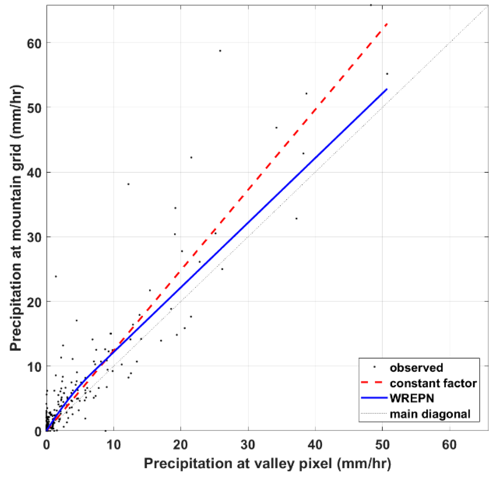
3.2. Results from the Elevation-Associated Rainfall Field Estimation Model

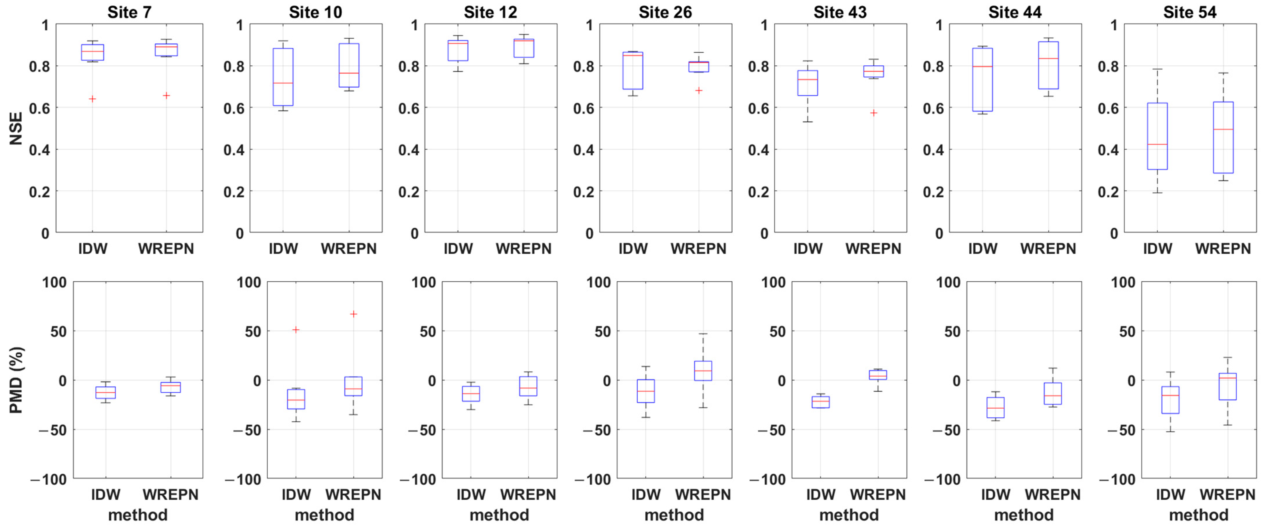
The data used to estimate the parameters of the proposed model are the rainfall fields of the WRF corresponding to the three storm events, which were bias-corrected by CM. The spatial resolution of the final domain of the WRF applied in this study is 3 km, resulting in a rainfall field consisting of pixels with 30 rows and 25 columns. The temporal resolution of the rainfall field is 1 h, and the total simulated time for the three storm events is 420 h.

Table 2. Topographic characteristics of pixel pairs.

No.	Pixel (Row, Column)	Station ID	Aspect	$∆\mathbf{x}$ (km)	$∆\mathbf{z}$ (m)
1	(18, 9) (17, 8)	KW 20184190	NW	4.2	689
2	(20, 4) (19, 4)	KW 20184210	N	3.0	458
3	(19,10) (20,11)	KW 20184260	SE	4.2	518
4	(19, 6) (18, 7)	MOE 20184150	NE	4.2	507
5	(7, 9) (8, 8)	AWS 914	SW	4.2	491
6	(21, 4) (22, 5)	AWS 945	NE	4.2	483
7	(21, 4) (22, 5)	AWS 791	SE	4.2	533
8	(22, 8) (23, 7)	AWS 906	SW	4.2	545

provides information of eight representative pixel pairs located in valleys and mountains, respectively. Representative pixel pairs were selected based on pixels with actual ground observation sites. The top pixel represents the mountain, while the bottom pixel represents the valley. Table 2 shows the inclination direction, horizontal distance difference, and vertical height difference in the WRF pixel system in addition to the observation site name. To examine the relationship between rainfall and elevation, it is crucial to select pixel pairs that represent the same aspect. The horizontal distance difference ($∆\mathrm{x}$) between the paired valley and mountain pixels was limited to within about 5 km, and the vertical elevation difference ($∆\mathrm{z}$) was limited to between 450 m and 750 m.

The increase in rainfall due to the mountain effect was analyzed for eight selected pixel pairs in valleys and mountains. The accumulated total rainfall in hourly timescale rainfall data is generally higher for mountain pixels than for valley pixels (

Table 3. Characteristics of rainfall between each pixel pair located at mountain and valley, including mean rainfall intensity and ratio of the mountain to valley rainfall totals (EF) during three storm events.

Pixel No.	Mean Rainfall Intensity (mm/h)		EF
	Mountain	Valley
1	3.6964	2.6149	1.4136
2	3.4747	3.0365	1.1443
3	4.1159	3.4185	1.2040
4	3.1409	2.7669	1.1352
5	2.5449	2.1138	1.2039
6	2.5439	2.2268	1.1424
7	3.6970	3.1600	1.1699
8	3.2974	2.6467	1.2458

). The difference in average rainfall intensity between mountain and valley pixels is 0.317–1.08 mm/h. When comparing the results of previous studies [29], this small difference may be attributed to the uncertainty of simulated precipitation by WRF. However, it is not appropriate to characterize this difference as being due to model uncertainty because the rainfall intensity at the mountain pixels is consistently greater than the rainfall intensity at the corresponding valley pixels. In Table 3, EF (Enhancement Factor) is defined as the relative ratio of average rainfall intensity between mountain and valley pixels depending on the change in terrain elevation. EF ranges from 1.14 to 1.41 for eight mountain-valley pixel pairs, all greater than 1.0. This means that rainfall intensity increases with increasing elevation.

The above analysis suggests that rainfall in the Namgang Dam watershed is influenced by the mountains. However, it is still difficult to model the rainfall–elevation relationship on the hourly timescale due to its complex variability. Figure 6 shows an example of a scatter plot of rainfall intensity in valleys and mountains using data from the first representative pixel pair. On the hourly timescale, the distribution of rainfall intensity is widely scattered. The figure suggests a weak linear relationship with a slope of about 1.24 (constant factor in Figure 6) for valley rainfall intensity up to about 50 mm/h. However, applying this relationship to all rainfall intensities overestimates the rainfall intensities of mountain pixels. Using a linear relationship, the total rainfall at the mountain pixel would be well reproducible, but conversely, it would underestimate the mountain effect for many rainfall intensities below about 10 mm/h at the valley pixel. For reference, WREPN in Figure 6 is an abbreviation of WRF Rainfall–Elevation Parameterized Nowcasting, and this represents the relationship between rainfall and elevation by the model proposed in this study.

The parameters of the proposed model were estimated using the data of eight pixel pairs in Table 2. For parameter estimation, the Markov Chain Monte Carlo (MCMC) algorithm, which can estimate the posterior distribution, was applied. As sampling algorithms, Metropolis–Hastings, Gibbs Sampling, Hamiltonian Monte Carlo, and No-U-Turn Sampler are widely used. In this study, the Metropolis–Hastings algorithm [35,36,37,38] was used, which is relatively simple and easy to apply and has a low computational cost compared to other algorithms in some cases. First, the values of the parameters estimated from the rainfall fields of two different storm events are presented in

Table 4. Estimated optimum parameter values for storm events.

Event	2003 and 2007	2007 and 2020	2020 and 2003	All Events
$\mathrm{a}$ (-)	1.62	1.65	1.55	1.65
$P_c$ (mm/h)	5.85	6.44	5.77	6.70

. It can be found that the difference in the values of the estimated parameters in each data set is not large. Finally, the rainfall fields of all three storm events were used to determine the values of the parameters (last column in Table 4). Sensitivity analysis for the parameters was not performed in this study and will be reviewed in a future study.

The rainfall fields considering the elevation effect were obtained from the proposed model using rainfall data in pixels with observation sites in the Namgang Dam watershed. Figure 7 shows the cumulative rainfall field simulated by WRF-CM for each storm event (left panel, WRF-CM), the cumulative rainfall field interpolated with IDW using rainfall data from pixels with observed sites (middle panel, IDW), and the cumulative rainfall field by the proposed model (right panel, WREPN), respectively. Figure 7 shows that the proposed model can be usefully applied to realize the spatial distribution of precipitation in mountainous areas. Comparison of IDW (Figure 7b,e,h) and WREPN (Figure 7c,f,i) in the region with high-elevation pixels and the region with low-elevation pixels reveals that the two rainfall fields are mostly similar in the low-elevation region. However, it can be said that the proposed model explains the rainfall fields better, as the rainfall field by WREPN in the high-elevation region is more similar to that of WRF-CM (Figure 7a,d,g). The increase in rainfall due to the mountain effect is evident with more rainfall in high mountains. In addition, rainfall distributions appear more realistic using an elevation-reflected algorithm that tracks along the terrain. In the low-lying area, there is little influence of elevation, so it is difficult to find the characteristics of the rainfall distribution. In fact, the Namgang Dam watershed has a relatively high density of rainfall observation networks compared to other areas in the Korea. The proposed model will play a more important role in representing the mountainous effect of rainfall in regions with low network density.

3.3. Validation

For validation of the proposed model, seven storm events that occurred in the past in the Namgang Dam watershed were used. The seven historical storm events used are summarized in

Table 5. Key specifications of storm events used for validation of the proposed model.

Event	The Time the Storm Event Occurred	Duration (h)	Rainfall Depth (mm)
1	1 August 2014 22:00	76	252
2	11 July 2015 14:00	49	172
3	27 August 2012 20:00	27	125
4	29 June 2018 21:00	103	156
5	21 August 2013 19:00	80	140
6	23 August 2018 01:00	39	102
7	19 August 2017 13:00	86	92

.

The validation method was performed using the concept of leave-one-out cross-validation (LOOCV) as follows.

(1) Excluding 1 site out of 55 sites.

(2) Calculate rainfall fields from IDW using data from sites other than the excluded site.

(2-1) Compare rainfall data observed at the excluded site with rainfall data interpolated from IDW at that site location.

(3) Calculate rainfall fields from the proposed model using data from sites other than the excluded site.

(3-1) Compare rainfall data observed at the excluded site with rainfall data simulated from WREPN at that site location.

(4) Repeatedly changing the excluded site.

Table 6. Specifications of sites in mountainous areas selected for validation of the proposed model.

No.	Site ID	Latitude (°)	Longitude (°)	Elevation (m)
7	KW20184210	127.5461	35.3469	630
10	KW20184240	127.7239	35.2842	660
12	KW20184260	127.7864	35.3147	640
26	MOE20184150	127.6419	35.3597	568
43	AWS315	127.5108	35.3067	1088
44	AWS872	127.7564	35.3192	869
54	AWS856	127.5982	35.1018	515

shows information about the sites selected for validation. The validation sites were selected from among the top 10 sites among the 55 sites applied in this study. Three of these ten sites were not suitable for performing validation due to intermittent missing data. The elevations of the selected sites ranged from 515 m to 1018 m.

As performance indicators for validation, Nash–Sutcliffe efficiency (NSE, [39]) and percent mean difference (PMD) were used. NSE is a representative performance index that evaluates the prediction performance of hydrologic models and is calculated as in the following Equation (6), and the closer it is to 1, the better the performance.

$$\mathrm{N}\mathrm{S}\mathrm{E}=1-\frac{{\sum }_{t=1}^T{\left(P_o\left(t\right)-P_s\left(t\right)\right)}^2}{{\sum }_{t=1}^T{(P_o(t)-\stackrel{-}{P_o})}^2}$$

(6)

where $\stackrel{-}{P_o}$ is the mean of observed rainfall data, and $P_s$ is simulated rainfall data. $P_o\left(t\right)$ is observed rainfall data at time $t$.

PMD is an index that evaluates the prediction performance of the total rainfall for each event at each site. It is calculated as Equation (7) below, and $\stackrel{-}{P_s}$ is the mean of simulated rainfall data. The closer it is to 0, the better the performance, and negative numbers indicate underestimation and positive numbers indicate overestimation.

$$\mathrm{P}\mathrm{M}\mathrm{D}=\frac{\stackrel{-}{P_s}-\stackrel{-}{P_o}}{\stackrel{-}{P_o}}\times 100$$

(7)

Figure 8 shows a box plot of performance index results for seven sites for each storm event. Although there are differences in the performance index for each storm event, the results show that WREPN performs relatively better than IDW. Based on the median value of NSE, WREPN predicts rainfall more accurately than IDW for all storm events at ungauged pixels. Both IDW and WREPN have a tendency to underestimate rainfall in mountainous areas (see PMD box plot in Figure 8). However, the data indicate that WREPN has the advantage of reducing this tendency of underestimation.

Figure 9 shows a box plot of performance index results for seven storm events for each site. Although there are differences in the performance index for each site, it can be seen that WREPN performs relatively better than IDW. Based on the median value of NSE, the prediction performance of WREPN is superior to that of IDW in all sites except Site 26. For reference, Site 26 is the second lowest elevation among the seven applied sites. At the highest elevation, Site 43, the NSE results indicate that WREPN accurately reflects the mountainous effect of rainfall in the Namgang Dam watershed, while IDW underestimates rainfall by more than 20% at Sites 10, 43, and 44 with relatively high elevation. However, WREPN significantly reduces the degree of underestimation at these sites. Additionally, WREPN slightly overestimates rainfall at Site 43.

Figure 10 shows the aggregated performance index of the LOOCV results for all storm events and all sites. Based on the median, WRPEN recognized that the NSE is 0.8 or more and can predict the rainfall in the mountainous area well. Additionally, PMD, which means percent error of total rainfall, shows performance within 5%. Figure 10 shows that the model proposed in this study adequately reflects the mountain effect of rainfall in the Namgang Dam watershed.

4. Conclusions

In this study, an algorithm was proposed to investigate the relationship between rainfall and elevation in the Namgang Dam watershed using high-resolution rainfall data from three storm events simulated by WRF and to consider the influence of elevation on hourly timescale rainfall. The simulation results of WRF confirmed an increase in rainfall due to the elevation effect in the Namgang Dam watershed. The analysis of eight representative pixel pairs in valleys and mountains suggests an increase in rainfall intensity for higher mountains. Rainfall data from eight representative pixel pairs were used to estimate the parameters of the proposed model. The proposed model shows parabolic increments for relatively small rainfall intensities and linear increments for relatively large rainfall intensities. It was confirmed that rainfall intensity in mountainous areas can be more realistically simulated using the algorithm that reflects the elevation effect compared with the result without elevation correction. This indicates that the proposed model can better estimate the spatial distribution of rainfall in the Namgang Dam watershed. Meanwhile, the proposed algorithm can be applied to the generation of real-time spatial rainfall distribution for flood prediction and warning in the Namgang Dam watershed. The results of leave-one-out cross-validation using seven storm events in the Namgang Dam watershed and seven sites in the mountainous area show that the proposed model can improve the prediction of rainfall intensity, especially in the mountainous area.

However, further studies are still needed to address some limitations of this study. Firstly, the present study considered the influence of elevation depending on the magnitude of rainfall intensity to minimize the computation time required for generating the real-time spatial rainfall field for flood forecasting and warning in terms of hydrology and disaster prevention. Since the actual relationship between rainfall and elevation is more complex, detailed physical analysis need to be conducted, and various environmental factors such as wind direction, thermal cycles, and mountain slope angle must be taken into account. Secondly, because the parameters of the proposed model were estimated based on rainfall data from only three storm events simulated by WRF, it is insufficient to generalize the results of this study. For practical applications, more storm events will be needed to accurately estimate model parameters. Finally, in the methodology proposed in this study, if there is an error in the simulation results of WRF, the reliability of the results will be significant affected. Although possible reliability was ensured through bias correction using ground observation data, a follow-up study using radar rainfall data that can provide detailed spatial information needs to be conducted. Additionally, because the focus of this study was on the amount of rainfall, additional physical analysis should be conducted through multidisciplinary cooperation to secure scientific validity. Given the characteristics of the Korea’s topography, which mostly consists of mountainous terrain, the effect of mountains on rainfall is an important topic for further study.

References

1. Smith, R.B. The Influence of Mountains on the Atmosphere. Adv. Geophys. 1979, 21, 87–230. [Google Scholar] [CrossRef]
2. Barry, R. Mountain Weather and Climate; Routledge: London, UK, 1992; 313p. [Google Scholar]
3. Basist, A.; Bell, G.D.; Meentemeyer, V. Statistical Relationships between Topography and Precipitation Patterns. J. Clim. 1994, 7, 1305–1315. [Google Scholar] [CrossRef]
4. Singh, P.; Kumar, N. Effect of orography on precipitation in the western Himalayan region. J. Hydrol. 1997, 199, 183–206. [Google Scholar] [CrossRef]
5. Weisse, A.K.; Bois, P. Topographic Effects on Statistical Characteristics of Heavy Rainfall and Mapping in the French Alps. J. Appl. Meteorol. Climatol. 2001, 40, 720–740. [Google Scholar] [CrossRef]
6. Pelosi, A.; Furcolo, P. An Amplification Model for the Regional Estimation of Extreme Rainfall within Orographic Areas in Campania Region (Italy). Water 2015, 7, 6877–6891. [Google Scholar] [CrossRef]
7. Li, Y.; Thompson, J.R.; Li, H. Impacts of Spatial Climatic Representation on Hydrological Model Calibration and Prediction Uncertainty: A Mountainous Catchment of Three Gorges Reservoir Region, China. Water 2016, 8, 73. [Google Scholar] [CrossRef]
8. Yang, M.; Zhang, W. Orographic Effects of Geomorphology on Precipitation in a Pluvial Basin of the Eastern Tibetan Plateau. Water 2019, 11, 250. [Google Scholar] [CrossRef]
9. Abbate, A.; Papini, M.; Longoni, L. Orographic Precipitation Extremes: An Application of LUME (Linear Upslope Model Extension) over the Alps and Apennines in Italy. Water 2022, 14, 2218. [Google Scholar] [CrossRef]
10. Auliagisni, W.; Wilkinson, S.; Elkharboutly, M. Learning from Floods—How a Community Develops Future Resilience. Water 2022, 14, 3238. [Google Scholar] [CrossRef]
11. Sein, Z.M.M.; Ullah, I.; Saleem, F.; Zhi, X.; Syed, S.; Azam, K. Interdecadal Variability in Myanmar Rainfall in the Monsoon Season (May–October) Using Eigen Methods. Water 2021, 13, 729. [Google Scholar] [CrossRef]
12. Haiden, T.; Pistotnik, G. Intensity-dependent parameterization of elevation effects in precipitation analysis. Adv. Geosci. 2009, 20, 33–38. [Google Scholar] [CrossRef]
13. Goovaerts, P. Geostatistical approaches for incorporating elevation into the spatial interpolation of rainfall. J. Hydrol. 2000, 228, 113–129. [Google Scholar] [CrossRef]
14. Guan, H.; Wilson, J.L.; Makhnin, O. Geostatistical Mapping of Mountain Precipitation Incorporating Autosearched Effects of Terrain and Climatic Characteristics. J. Hydrometeorol. 2005, 6, 1018–1031. [Google Scholar] [CrossRef]
15. Hunter, R.D.; Meentemeyer, R. Climatologically Aided Mapping of Daily Precipitation and Temperature. J. Appl. Meteorol. Climatol. 2005, 44, 1501–1510. [Google Scholar] [CrossRef]
16. Daly, C.; Neilson, R.; Phillips, D. A statistical-topographic model for mapping climatological precipitation over mountainous terrain. J. Appl. Meteorol. Climatol. 1994, 33, 140–158. [Google Scholar] [CrossRef]
17. Sharples, J.J.; Hutchinson, M.F.; Jellett, D.R. On the Horizontal Scale of Elevation Dependence of Australian Monthly Precipitation. J. Appl. Meteorol. Climatol. 2005, 44, 1850–1865. [Google Scholar] [CrossRef]
18. Ohara, N.; Kavvas, M.L.; Kure, S.; Chen, Z.Q.; Jang, S.; Tan, E. Physically Based Estimation of Maximum Precipitation over American River Watershed, California. J. Hydrol. Eng. 2011, 16, 351–361. [Google Scholar] [CrossRef]
19. Grell, G.A.; Dudhia, J.; Stauffer, D.R. A Description of the Fifth-Generation Penn State/NCAR Mesoscale Model (MM5) (No. NCAR/TN-398+STR); University Corporation for Atmospheric Research: Boulder, CO, USA, 1994. [Google Scholar] [CrossRef]
20. Wu, M.-C.; Yang, S.-C.; Yang, T.-H.; Kao, H.-M. Typhoon Rainfall Forecasting by Means of Ensemble Numerical Weather Predictions with a GA-Based Integration Strategy. Atmosphere 2018, 9, 425. [Google Scholar] [CrossRef]
21. Karki, R.; Hasson, S.U.; Gerlitz, L.; Talchabhadel, R.; Schenk, E.; Schickhoff, U.; Scholten, T.; Böhner, J. WRF-based simulation of an extreme precipitation event over the Central Himalayas: Atmospheric mechanisms and their representation by microphysics parameterization schemes. Atmos. Res. 2018, 214, 21–35. [Google Scholar] [CrossRef]
22. Patel, P.; Ghosh, S.; Kaginalkar, A.; Islam, S.; Karmakar, S. Performance evaluation of WRF for extreme flood forecasts in a coastal urban environment. Atmos. Res. 2019, 223, 39–48. [Google Scholar] [CrossRef]
23. Caumont, O.; Mandement, M.; Bouttier, F.; Eeckman, J.; Brossier, C.L.; Lovat, A.; Nuissier, O.; Laurantin, O. The heavy precipitation event of 14–15 October 2018 in the Aude catchment: A meteorological study based on operational numerical weather prediction systems and standard and personal observations. Nat. Hazards Earth Syst. Sci. 2021, 21, 1135–1157. [Google Scholar] [CrossRef]
24. Jankov, I.; Schultz, P.J.; Anderson, C.J.; Koch, S.E. The Impact of Different Physical Parameterizations and Their Interactions on Cold Season QPF in the American River Basin. J. Hydrometeorol. 2007, 8, 1141–1151. [Google Scholar] [CrossRef]
25. Hong, S.-Y.; Lee, J.-W. Assessment of the WRF model in reproducing a flash-flood heavy rainfall event over Korea. Atmos. Res. 2009, 93, 818–831. [Google Scholar] [CrossRef]
26. Baik, J.; Park, J.; Rye, D.; Choi, M. Geospatial blending to improve spatial mapping of precipitation with high spatial resolution by merging satellite-based and ground-based data. Hydrol. Process. 2016, 30, 2789–2803. [Google Scholar] [CrossRef]
27. Haiden, T.; Kann, A.; Pistotnik, G.; Standlbacher, K.; Wittmann, C. Integrated Nowcasting through Comprehensive Analysis (INCA)—System Description; ZAMG Report; Zentralanstalt für Meteorologie und Geodynamik: Vienna, Austria, 2009; 60p. [Google Scholar]
28. Ghaemi, E.; Foelsche, U.; Kann, A.; Fuchsberger, J. Evaluation of Integrated Nowcasting through Comprehensive Analysis (INCA) precipitation analysis using a dense rain-gauge network in southeastern Austria. Hydrol. Earth Syst. Sci. 2021, 25, 4335–4356. [Google Scholar] [CrossRef]
29. Song, L.; Chen, M.; Gao, F.; Cheng, C.; Chen, M.; Yang, L.; Wang, Y. Elevation Influence on Rainfall and a Parameterization Algorithm in the Beijing Area. J. Meteorol. Res. 2019, 33, 1143–1156. [Google Scholar] [CrossRef]
30. Lee, J.; Choi, J.; Jeong, H.; Kim, S. Preliminary Study for Physically Based Estimation of Maximum Precipitation Using the Regional Climate Model in Korea: Reconstruction of Typhoon RUSA Rainfall. J. Korean Soc. Hazard Mitig. 2017, 17, 401–411. (In Korean) [Google Scholar] [CrossRef]
31. Choi, J.; Lee, J.; Jeong, H.-G.; Jang, J.; Kim, S. Effect of Improvement of Initial and Boundary Conditions in WRF Model on Simulating Typhoon Rainfall. J. Korean Soc. Hazard Mitig. 2018, 18, 445–454. (In Korean) [Google Scholar] [CrossRef]
32. Choi, J.; Lee, O.; Jang, S.; Jo, D.-J.; Kim, S. Effect of Sea Surface Temperature on Maximizing Typhoon Rainfall Depth. J. Korean Soc. Hazard Mitig. 2018, 18, 443–452. (In Korean) [Google Scholar] [CrossRef]
33. Won, J.; Choi, J.; Lee, O.; Kim, S. Evaluation of Rainfall-Event-Simulation Performance of the WRF Model Combined with ERA-Interim Data: Focus on the Rainfall Event in Imjin River Basin in 1999. J. Korean Soc. Hazard Mitig. 2019, 19, 205–213. (In Korean) [Google Scholar] [CrossRef]
34. Lee, J.; Choi, J.; Lee, O.; Kim, S. Reconstruction of July 2006 Heavy Rainfall Event Series in the Chungju Dam Watershed using a Regional Climate Model. J. Korean Soc. Hazard Mitig. 2019, 19, 331–338. (In Korean) [Google Scholar] [CrossRef]
35. Metropolis, N.; Rosenbluth, A.W.; Rosenbluth, M.N.; Teller, A.H.; Teller, E. Equation of State Calculations by Fast Computing Machines. J. Chem. Phys. 1953, 21, 1087–1092. [Google Scholar] [CrossRef]
36. Hastings, W.K. Monte Carlo Sampling Methods Using Markov Chains and Their Applications. Biometrika 1970, 57, 97–109. [Google Scholar] [CrossRef]
37. Lee, O.; Choi, J.; Won, J.; Kim, S. Uncertainty in nonstationary frequency analysis of South Korea’s daily rainfall peak over threshold excesses associated with covariates. Hydrol. Earth Syst. Sci. 2020, 24, 5077–5093. [Google Scholar] [CrossRef]
38. Lee, O.; Seo, J.; Won, J.; Choi, J.; Kim, S. Future extreme heat wave events using Bayesian heat wave intensity-persistence day-frequency model and their uncertainty. Atmos. Res. 2021, 255, 105541. [Google Scholar] [CrossRef]
39. Nash, J.E.; Sutcliffe, J.V. River flow forecasting through conceptual models part I—A discussion of principles. J. Hydrol. 1970, 10, 282–290. [Google Scholar] [CrossRef]
Figure 1. Schematic diagram for research.
Water 15 01794 g001
Figure 2. Target area and ground rainfall observation sites.
Water 15 01794 g002
Figure 3. WRF model domain for rainfall simulation.
Water 15 01794 g003
Figure 4. Cumulative rainfall depth by spatial rainfall field estimation for three storm events. (a1a3) Kriging results based on ground observation data, (b1b3) WRF original result, (c1c3) WRF result with bias correction using CM technique.
Water 15 01794 g004
Figure 5. Temporal distribution of spatially averaged rainfall intensity for three storm events.
Water 15 01794 g005
Figure 6. Scatter plot of hourly rainfall intensities at the valley and mountain for first pixel pair.
Water 15 01794 g006
Figure 7. Cumulative rainfall field by storm event according to spatial rainfall field estimation method. (a) WRF-CM result for Event 2003, (b) IDW result for Event 2003, (c) WREPN result for Event 2003, (d) WRF-CM result for Event 2007, (e) IDW result for Event 2007, (f) WREPN result for Event 2007, (g) WRF-CM result for Event 2020, (h) IDW result for Event 2020, (i) WREPN result for Event 2020.
Water 15 01794 g007
Figure 8. Performance index results for seven sites for each storm event through LOOCV analysis.
Water 15 01794 g008
Figure 9. Performance index results for seven storm events for each site through LOOCV analysis.
Water 15 01794 g009
Figure 10. Aggregated performance index results using LOOCV analysis for all storm events and all sites.
Water 15 01794 g010