


Construction of an Agricultural Drought Monitoring Model for Karst with Coupled Climate and Substratum Factors—A Case Study of Guizhou Province, China
Abstract
:1. Introduction
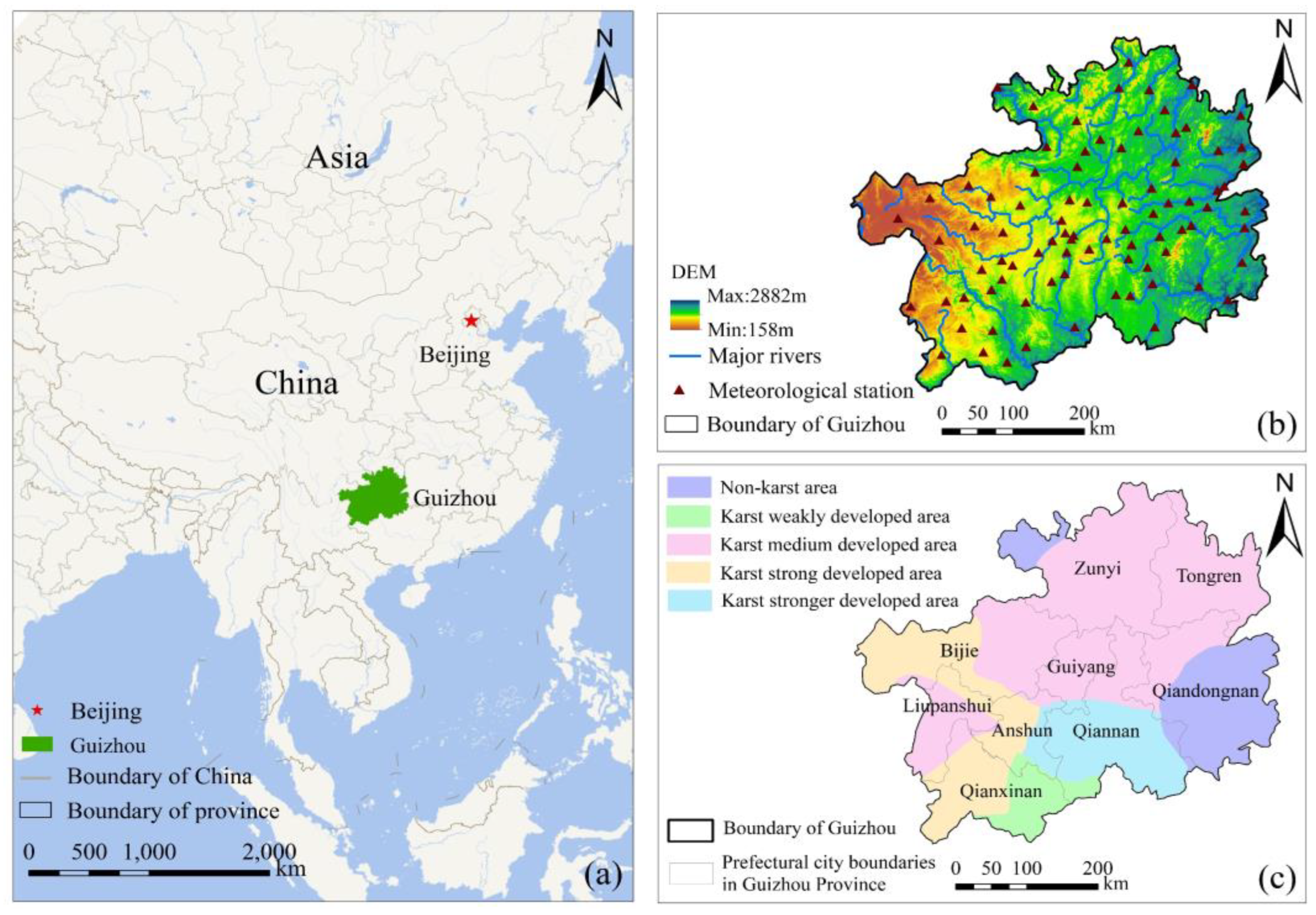
2. Study Area
3. Materials and Methods
3.1. Data Source and Pre-Processing
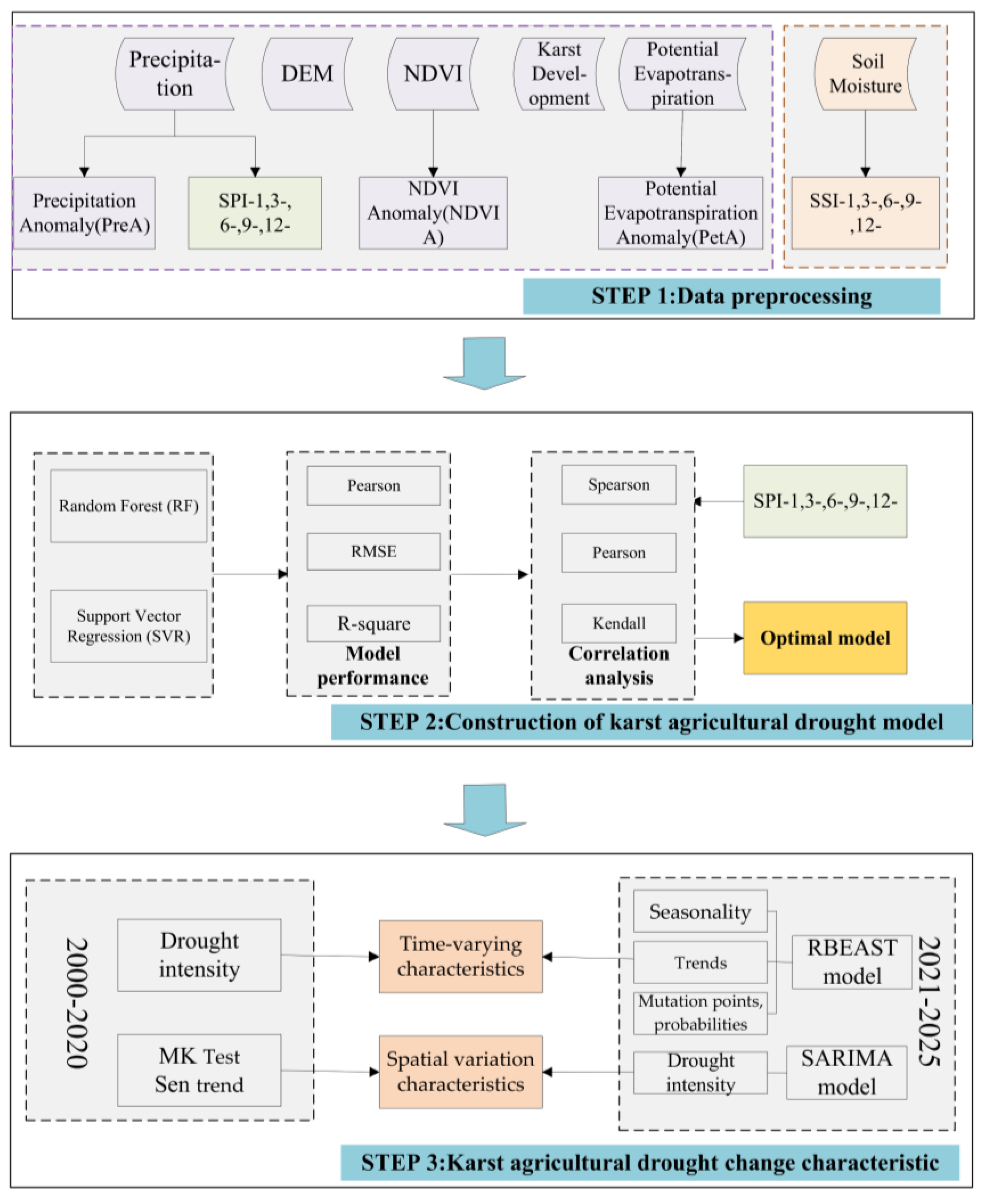
3.2. Research Methodology
3.2.1. Drought Identification
3.2.2. Karst Agricultural Drought Model Construction
- (1)
- Model construction
- (2)
- RF model construction
- (3)
- SVR model construction
- (4)
- Evaluation model method
3.2.3. Drought Prediction
3.2.4. Other Methods
4. Results and Analysis
4.1. Performance Evaluation of the Karst Agricultural Drought Monitoring Model
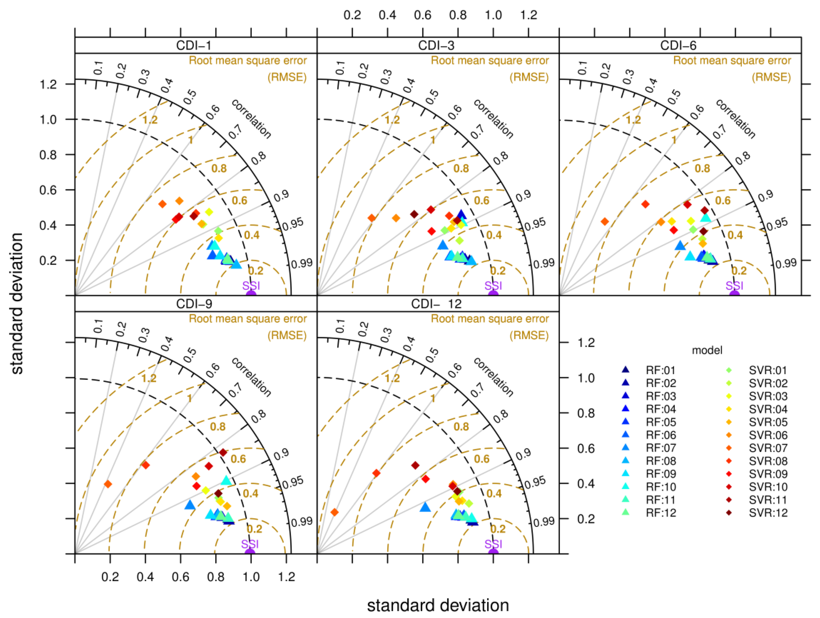
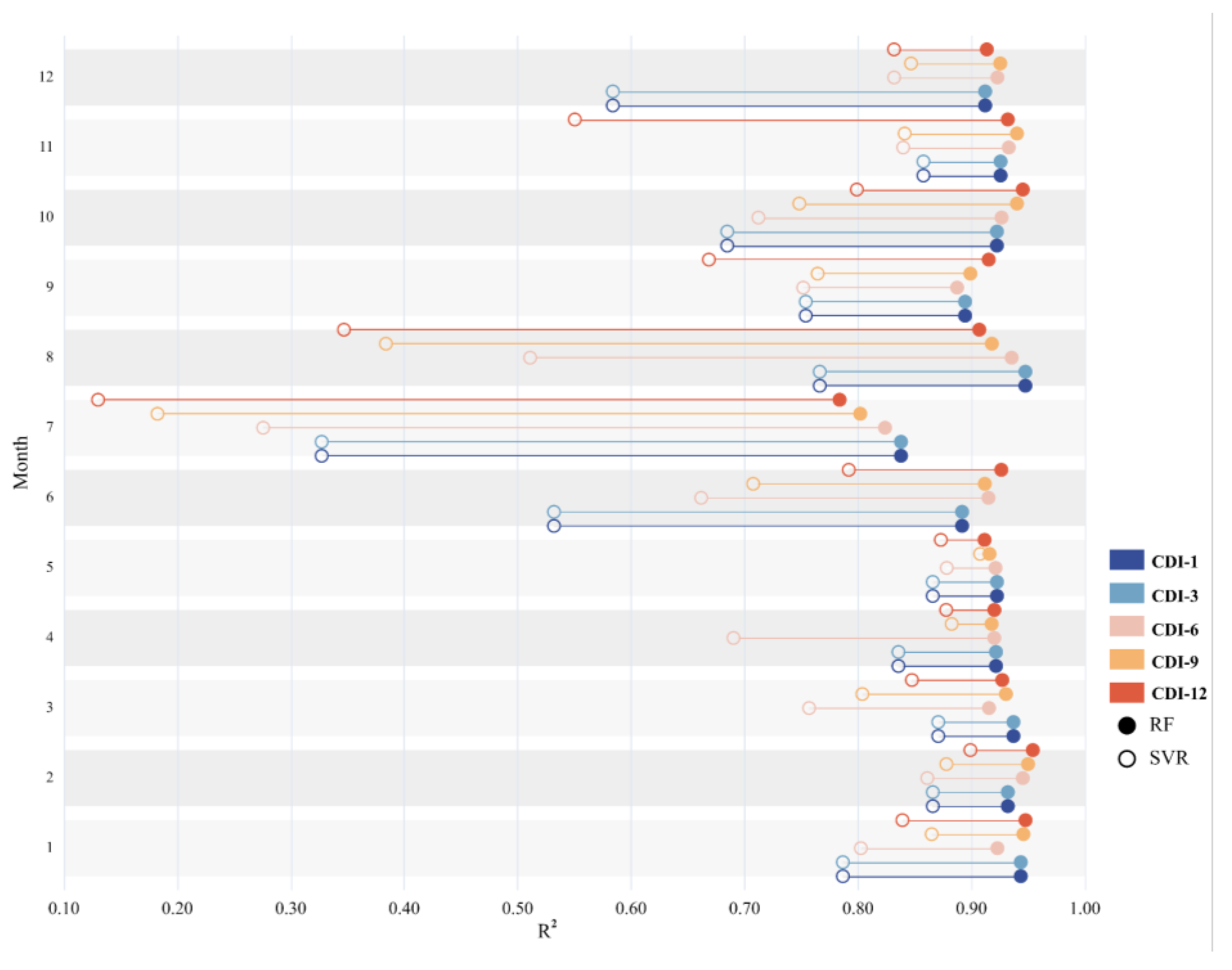
4.1.1. Model Validation and Evaluation
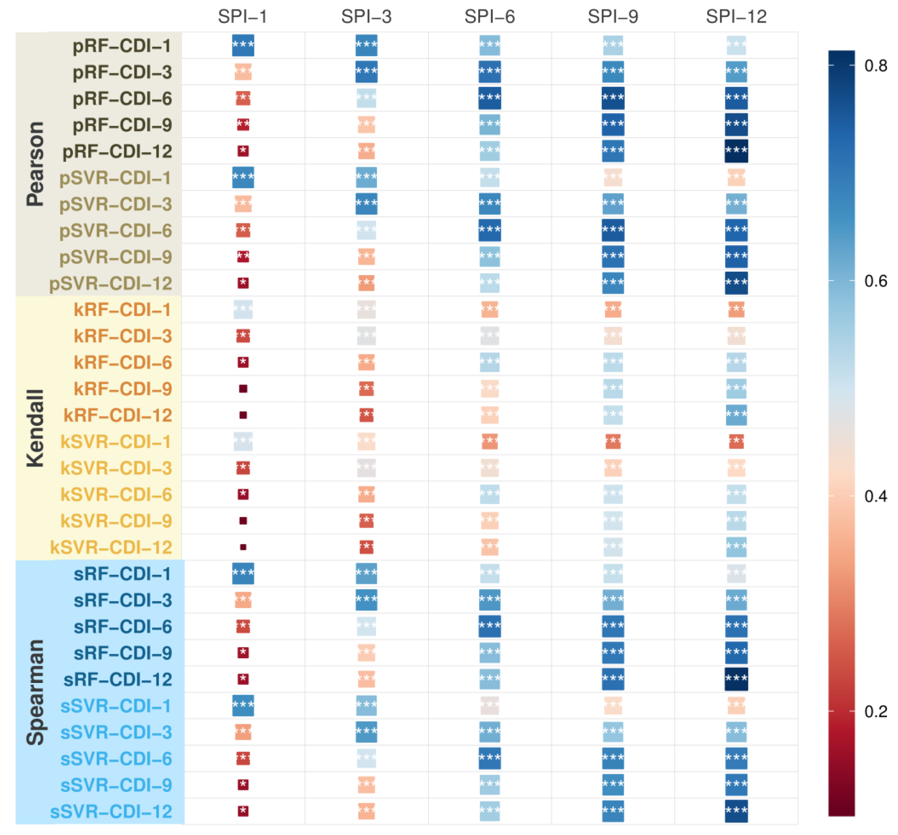
4.1.2. Correlation Metric of RF-CDI, SVR-CDI, and SPI
4.2. Analysis of Karst Agricultural Drought Change Characteristics
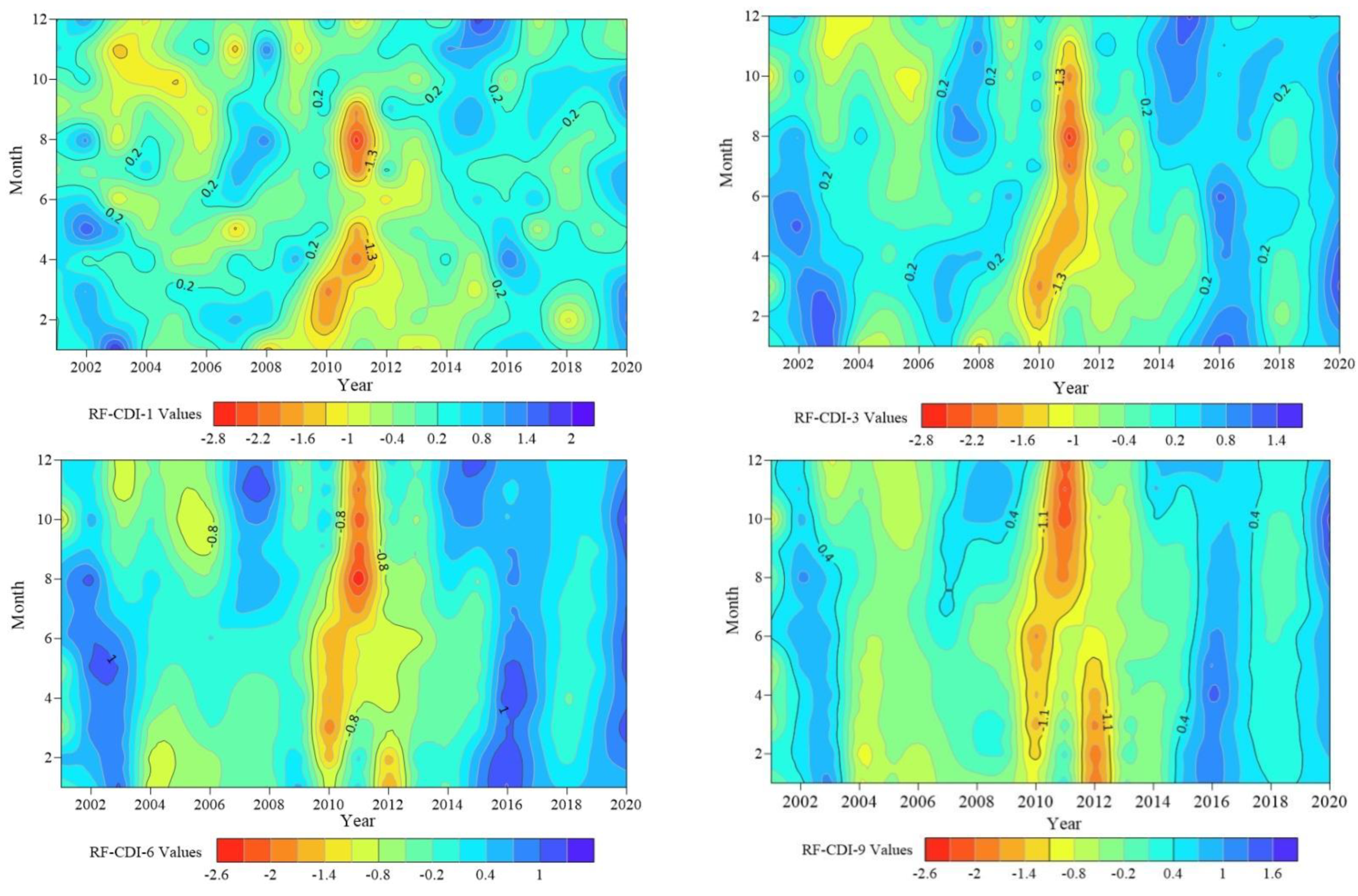
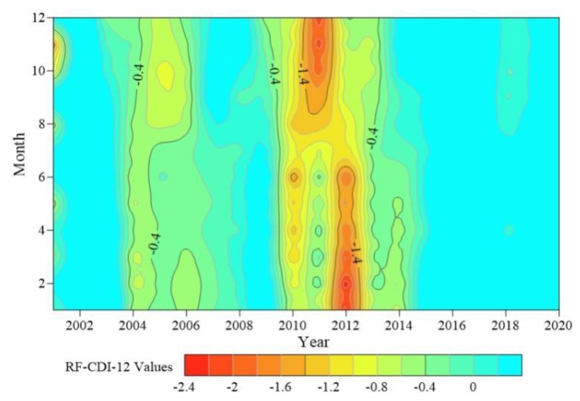
4.2.1. Time-Varying Characteristics
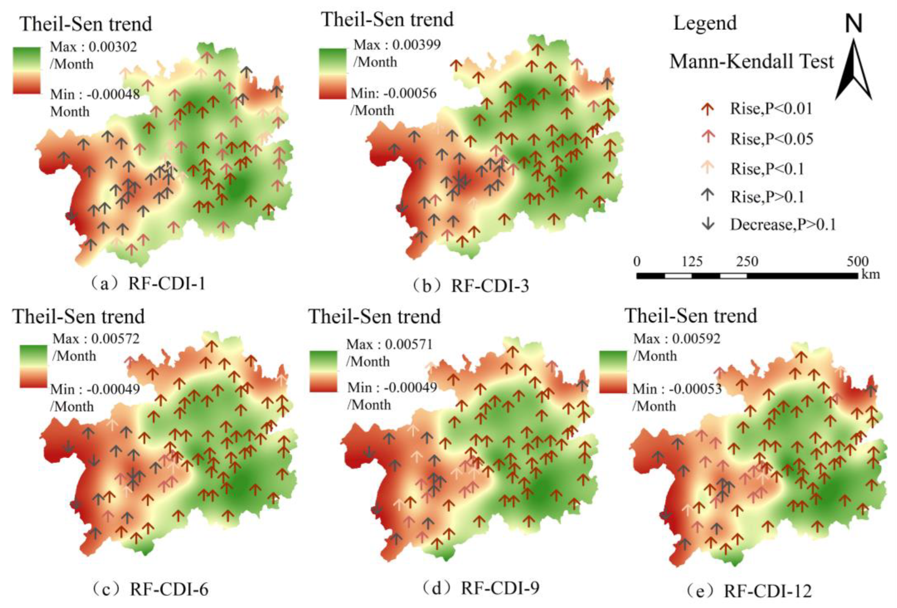
4.2.2. Spatial Variation Characteristics
4.3. Karst Agricultural Drought Forecast for the Next 5 Years
4.3.1. Spatial Distribution Characteristics of Karst Agricultural Drought in the Next 5 Years
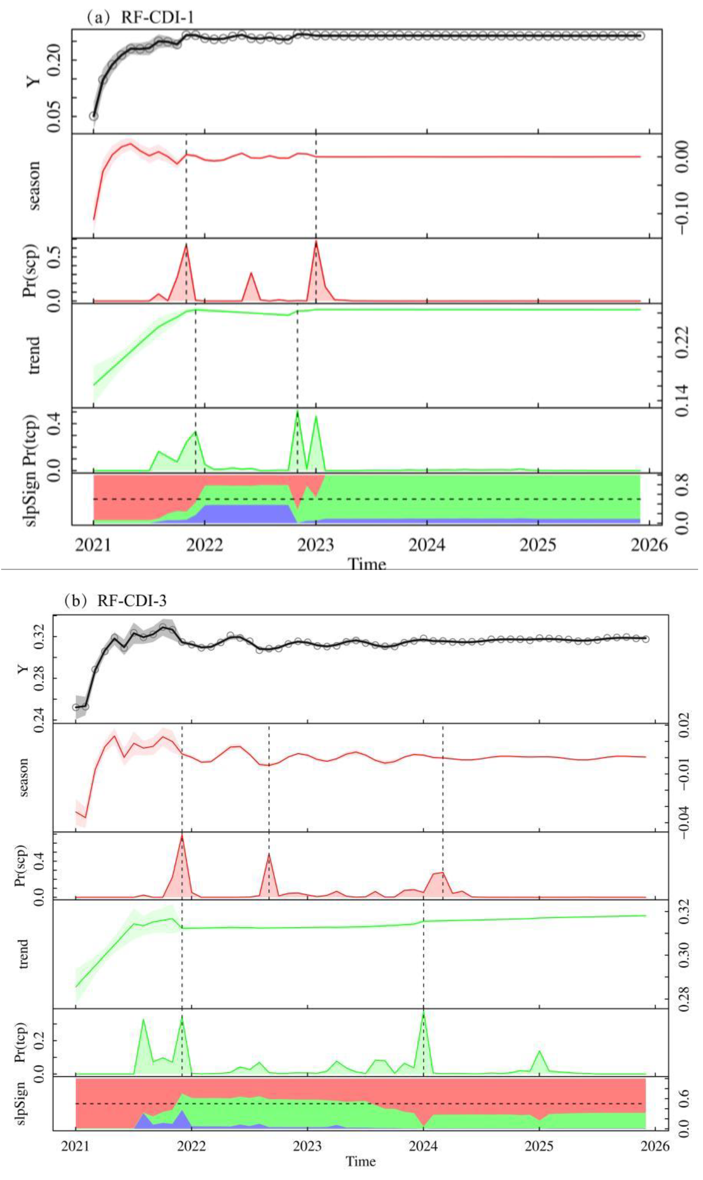
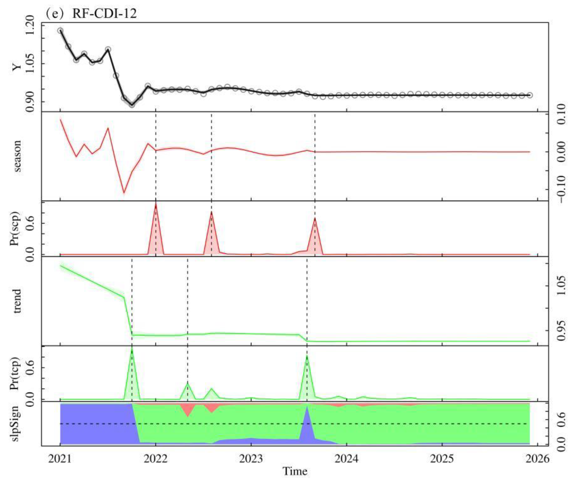
4.3.2. Characteristics of Temporal Changes of Karst Agricultural Drought for the Next 5 Years
5. Discussion
6. Conclusions
Author Contributions
Funding
Data Availability Statement
Conflicts of Interest
References
- Zhou, K.K.; Li, J.Z.; Zhang, T.; Kang, A. The use of combined soil moisture data to characterize agricultural drought conditions and the relationship among different drought types in China. Agric. Water Manag. 2021, 243, 106479–106493. [Google Scholar] [CrossRef]
- Mishra, A.K.; Singh, V.P. A review of drought concepts. J. Hydrol. 2010, 391, 202–216. [Google Scholar] [CrossRef]
- Alzira, G.S.S.S.; Alfredo, R.N.; Laio, L.D.S. Soil moisture-based index for agricultural drought assessment: SMADI application in Pernambuco State-Brazil. Remote Sens. Environ. 2021, 252, 112124–112139. [Google Scholar]
- Sandeep, P.; Obi, R.G.P.; Jegankumar, R.; Arun, K.C. Monitoring of agricultural drought in semi-arid ecosystem of Peninsular India through indices derived from time-series CHIRPS and MODIS datasets. Ecol. Indic. 2021, 121, 107033. [Google Scholar] [CrossRef]
- Liu, X.F.; Zhu, X.F.; Pan, Y.Z.; Li, S.; Liu, Y.; Ma, Y. Agricultural drought monitoring:progress, challenges, and prospects. J. Geogr. Sci. 2016, 26, 750–767. [Google Scholar] [CrossRef]
- Dai, A.; Trenberth, K.E.; Qian, T.T. A Global Dataset of Palmer Drought Severity Index for 1870–2002: Relationship with Soil Moisture and Effects of Surface Warming. J. Am. Meteorol. Soc. 2004, 5, 1117–1130. [Google Scholar] [CrossRef]
- Kogan, F.N. Remote sensing of weather impacts on vegetation in non-homogeneous areas. Int. J. Remote Sens. 2007, 11, 1405–1419. [Google Scholar] [CrossRef]
- Kogan, F.N. Application of vegetation index and brightness temperature for drought detection. Adv. Space Res. 1995, 15, 91–100. [Google Scholar] [CrossRef]
- Zhang, A.Z.; Gensuo, J. Monitoring meteorological drought in semiarid regions using multi-sensor microwave remote sensing data. Remote Sens. Environ. 2013, 134, 12–23. [Google Scholar] [CrossRef]
- Albert, I.J.M.V.D.; Beck, H.E.; Crosbie, R.S. The millennium drought in southeast Australia (2001–2009): Natural and human causes and implications for water resources, ecosystems, economy, and society. Water Resour. Res. 2013, 49, 1040–1057. [Google Scholar]
- Tadesse, T.; Champagne, C.; Wardlow, B.D.; Hadwen, T.A.; Brown, J.F.; Demisse, G.B.; Davidson, A.M. Building the vegetation drought response index for Canada (VegDRI-Canada) to monitor agricultural drought: First results. GISci. Remote Sens. 2017, 54, 230–257. [Google Scholar] [CrossRef]
- Sun, L.; Wang, F.; Li, B.G.; Chen, X. Study on drought monitoring of wuling mountain area based on multi-source data. Trans. Chin. Soc. Agric. Mach. 2014, 45, 246–252. [Google Scholar]
- Rhee, J.; Im, J.; Carbone, G.J. Monitoring agricultural drought for arid and humid regions using multi-sensor remote sensing data. Remote Sens. Environ. 2010, 114, 2875–2887. [Google Scholar] [CrossRef]
- Brown, J.F.; Wardlow, B.D.; Tadesse, T.; Hayes, M.J.; Reed, B.C. The vegetation drought response index (VegDRI): A new integrated approach for monitoring drought stress in vegetation. GISci. Remote Sens. 2008, 45, 16–46. [Google Scholar] [CrossRef]
- Wu, J.J.; Zhou, L.; Liu, M.; Zhang, J.; Leng, S.; Diao, C. Establishing and assessing the Integrated Surface Drought Index (ISDI) for agricultural drought monitoring in Mid-Eastern China. Int. J. Appl. Earth Obs. Geoinf. 2013, 23, 397–410. [Google Scholar] [CrossRef]
- Du, L.T.; Tian, Q.J.; Yu, T.; Meng, Q.; Jancso, T.; Udvardy, P.; Huang, Y. A comprehensive drought monitoring method integrating MODIS and TRMM data. Int. J. Appl. Earth Obs. Geoinf. 2012, 23, 245–253. [Google Scholar] [CrossRef]
- Shen, R.P.; Gou, J.; Li, L.X. Construction of a drought monitoring model using the random forest based remote sensing. J. Geo-Inf. Sci. 2017, 19, 125–133. [Google Scholar]
- Han, L.Y.; Zhang, Q.; Ma, P.L.; Jia, J.; Wang, J. The spatial distribution characteristics of a comprehensive drought risk index in southwestern China and underlying causes. Theor. Appl. Climatol. 2016, 124, 517–528. [Google Scholar] [CrossRef]
- Li, K.Z.; Xu, Z.C.; Lv, X.X.; Dong, Y.P.; Wang, H.S. Quantifying the effect of drought with different durations on karst dissolution based on field control test. Prog. Geogr. 2021, 40, 1704–1715. [Google Scholar] [CrossRef]
- Chen, L.H.; He, Z.H.; Pan, S. Spatial and Temporal Evolution Characteristics of Karst Agricultural Drought Based on Different Time Scales and Driving Detection. J. Soil Water Conserv. 2023, 37, 136–148. [Google Scholar]
- Zhao, Y.L.; Zhao, J.; Li, Y.; Xue, Q.Y. Research progress of Huajiang Kaest gorge, Cuizhou Province. J. Guizhou Norm. Univ. 2022, 40, 1–10+132. [Google Scholar]
- Huang, D.H.; Zhou, Z.F.; Peng, R.W.; Zhu, M.; Yin, L.J.; Zhang, Y.; Xiao, D.N.; Li, Q.X.; Hu, L.W.; Huang, Y.Y. Challenges and main research advances of low-altitude remote sensing for crops in southwest plateau mountains. J. Guizhou Norm. Univ. 2021, 39, 51–59. [Google Scholar]
- Oroian, M.; Dranca, F.; Ursachi, F. Comparative evaluation of maceration, microwave and ultrasonic-assisted extraction of phenolic compounds from propolis. J. Food Sci. Technol. 2020, 57, 70–78. [Google Scholar] [CrossRef] [PubMed]
- Mansoor, Z.; Bahram, S.; Majid, D. Probabilistic hydrological drought index forecasting based on meteorological drought index using Archimedean copulas. Hydrol. Res. 2019, 50, 1230–1250. [Google Scholar]
- Wen, Q.Z.; Sun, P.; Zhang, Q.; Liu, J.M.; Shi, P.J. An integrated agricultural drought monitoring model based on multi-source Remote Sensing data: Model development and application. Acta Ecol. Sin. 2019, 39, 7757–7770. [Google Scholar]
- Du, L.T.; Tian, Q.J.; Wang, L.; Huang, Y.; Nan, L. A synthesized drought monitoring model based on multi-source remote sensing data. Trans. Chin. Soc. Agric. Eng. 2014, 30, 126–132. [Google Scholar]
- Breiman, L. Random forests. Mach. Learn. 2001, 45, 5–32. [Google Scholar] [CrossRef]
- Zhou, Y.Y.; Fu, D.J.; Lu, C.X.; Xu, X.; Tang, Q. Positive effects of ecological restoration policies on the vegetation dynamics in a typical ecologically vulnerable area of China. Ecol. Eng. 2021, 159, 106087. [Google Scholar] [CrossRef]
- Sain, S.R. The Nature of Statistical Learning Theory. Technometrics 2012, 38, 409. [Google Scholar] [CrossRef]
- Tian, Y.; Wang, X.Y.; Ping, G.Q. Agricultural drought prediction using climate indices based on Support Vector Regression in Xiangjiang River basin. Sci. Total Environ. 2018, 622, 710–720. [Google Scholar] [CrossRef]
- Ding, Y.L.; Zhang, H.Y.; Wang, Z.Q.; Xie, Q.; Wang, Y.; Liu, L.; Hall, C.C. A Comparison of Estimating Crop Residue Cover from Sentinel-2 Data Using Empirical Regressions and Machine Learning Methods. Remote Sens. 2020, 12, 1470. [Google Scholar] [CrossRef]
- Yang, L.P.; Ren, J.; Wang, Y.; Zhang, J.; Wang, T.; Li, K.X. Soil salinity estimation model in Juyanze based on multi-source remote sensing data. Trans. Chin. Soc. Agric. Mach. 2022, 53, 226–235. [Google Scholar]
- Ediger, V.Ş.; Akar, S.; Uğurlu, B. Forecasting production of fossil fuel sources in Turkey using a comparative regression and ARIMA model. Energy Policy 2006, 34, 3836–3846. [Google Scholar] [CrossRef]
- Tan, X.J.; Zheng, Q.Y. Dynamic analysis and forecast of water resources ecological footprint in China. Acta Ecol. Sin. 2009, 29, 3559–3568. [Google Scholar]
- Patrícia, R.; Nicolau, S.; Rui, R. Performance of state space and ARIMA models for consumer retail sales forecasting. Robot. Comput. Integr. Manuf. 2015, 34, 151–163. [Google Scholar]
- Bouzerdoum, M.; Mellit, A.; Massi, P.A. A hybrid model (SARIMA–SVM) for short-term power forecasting of a small-scale grid-connected photovoltaic plant. Sol. Energy 2013, 98, 226–235. [Google Scholar] [CrossRef]
- Sbabel, A.; Fukushi, K.; Sitanrassamee, B. Effect of acid speciation on solid waste liquefaction in an anaerobic acid digester. Water Res. 2004, 38, 2416–2422. [Google Scholar]
- Ren, S.S.; Gao, M.; Wang, X.W.; Yu, Y.q.; Chen, J.X.; Chen, N. Algal bloom prediction in the Jiulong River Reservoir based on three types of time series models. Acta Sci. Circumst. 2022, 42, 172–183. [Google Scholar]
- Kumar, P.S. Estimates of the regression coefficient based on Kendall’s Tau. J. Am. Stat. Assoc. 1968, 63, 1379–1389. [Google Scholar]
- Liang, D.L.; Tang, H.P. Analysis of vegetation changes and water temperature driving factors in two apling grasslands on the Qinghai-Tibet Plateau. Acta Ecol. Sin. 2022, 42, 287–300. [Google Scholar]
- White, J.H.R.; Walsh, J.E. Using Bayesian statistics to detect trends in Alaskan precipitation. Int. J. Climatol. 2020, 41, 2045–2059. [Google Scholar] [CrossRef]
- Hu, T.X.; Myers, T.E.; Chen, G.; Toman, E.M.; Shao, G.; Zhao, Y.; Li, Y.; Zhao, K.; Feng, Y. Mapping fine-scale human disturbances in a working landscape with Landsat time series on Google Earth Engine. ISPRS J. Photogramm. Remote Sens. 2021, 176, 250–261. [Google Scholar] [CrossRef]
- Zhao, K.G.; Hu, T.X.; Wulder, M.A.; Bright, R.; Wu, Q.; Qin, H.; Li, Y.; Toman, E.; Mallick, B.; Zhang, X.; et al. Detecting change-point, trend, and seasonality in satellite time series data to track abrupt changes and nonlinear dynamics: A bayesian ensemble algorithm. Remote Sens. Environ. 2019, 232, 111181–111201. [Google Scholar] [CrossRef]
- Olusola, O.A.; Yi, L.; Songbai, S.; Ning, Y. Spatial comparability of drought characteristics and related return periods in China’s mainland over 1961–2013. J. Hydrol. 2017, 550, 549–567. [Google Scholar]
- Van, L.A.F.; Van, H.M.H.J.; Van, L.H.A.J. Evaluation of drought propagation in an ensemble mean of large-scale hydrological models. Hydrol. Earth Syst. Sci. 2012, 16, 4057–4078. [Google Scholar]
- Woodward, F.I.; Lomas, M.R.; Kelly, C.K. Global climate and the distribution of plant biomes. Philos. Trans. R. Soc. Lond. Ser. B Biol. Sci. 2004, 359, 1465–1476. [Google Scholar] [CrossRef]
- He, Z.H.; Chen, X.X.; Liang, H. Studies on the mechanism of watershed hydrologic droughts based on the combined structure of typical karst lithologys:taking Cuizhou province as a case. Chin. J. Geol. 2015, 50, 340–353. [Google Scholar]
- Xiong, K.N.; Zhu, D.Y.; Peng, T.; Yu, L.F.; Xue, J.H.; Li, P. Study on ecological industry technology and demonstration for Karst Rocky desertification control of the Karst Plateau-Gorge. Acta Ecol. Sin. 2016, 36, 7109–7113. [Google Scholar]
- Pi, G.N.; He, Z.H.; Zhang, L.; Yang, M.K.; You, M. Response of vegetation to meteorological drought in watershed at different time scales—A case study of Guizhou Province. Res. Soil Water Conserv. 2022, 29, 277–284+291. [Google Scholar]
- Hu, X.P.; Wang, S.G.; Xu, P.P.; Shang, K.Z. Analysis on causes of continuous drought in Southwest China during 2009–2013. Meteorol. Mon. 2014, 40, 1216–1229. [Google Scholar]
- Wang, S.; Li, R.P.; Li, X.Z. Inversion and distribution of soil moisture in belly of Maowusu sandy land based on comprehensive drought index. Trans. Chin. Soc. Agric. Eng. 2019, 35, 113–121. [Google Scholar]
- Han, Z.M.; Huang, Q.; Huang, S.Z.; Leng, G.; Bai, Q.; Liang, H.; Wang, L.; Zhao, J.; Fang, W. Spatial-temporal dynamics of agricultural drought in the Loess Plateau under a changing environment: Characteristics and potential influencing factors. Agric. Water Manag. 2021, 244, 106540–106552. [Google Scholar] [CrossRef]


| SPI|SSI | Drought Level |
|---|---|
| Normal | |
| Light | |
| Moderate | |
| Severe | |
| Extreme |
| January | February | March | April | May | June | July | August | September | October | November | December | |
|---|---|---|---|---|---|---|---|---|---|---|---|---|
| RF-CDI1 | 1505 | 1802 | 538 | 280 | 1700 | 2000 | 1887 | 378 | 165 | 578 | 345 | 819 |
| RF-CDI3 | 473 | 294 | 679 | 1888 | 374 | 1993 | 1499 | 1701 | 180 | 1056 | 1271 | 806 |
| RF-CDI6 | 533 | 1449 | 1983 | 995 | 1963 | 1967 | 673 | 944 | 1048 | 1916 | 1962 | 533 |
| RF-CDI9 | 334 | 1990 | 1475 | 1410 | 1797 | 1411 | 1809 | 1980 | 324 | 1194 | 1988 | 245 |
| RF-CDI12 | 308 | 1349 | 1656 | 669 | 1656 | 1092 | 822 | 822 | 837 | 1092 | 1994 | 241 |
| January | February | March | April | May | June | July | August | September | October | November | December | ||
|---|---|---|---|---|---|---|---|---|---|---|---|---|---|
| SVR-CDI1 | gamma | 2 | 1 | 1 | 2 | 1 | 1 | 0.1 | 0.1 | 1 | 1 | 1 | 1 |
| cost | 3 | 2 | 2 | 2 | 1 | 2 | 1 | 4 | 2 | 1 | 1 | 1 | |
| SVR-CDI3 | gamma | 3 | 3 | 3 | 2 | 2 | 2 | 0.1 | 1 | 4 | 1 | 4 | 1 |
| cost | 1 | 2 | 2 | 2 | 3 | 1 | 1 | 4 | 2 | 1 | 2 | 1 | |
| SVR-CDI6 | gamma | 3 | 2 | 2 | 1 | 3 | 2 | 0.1 | 0.1 | 4 | 1 | 3 | 4 |
| cost | 2 | 2 | 2 | 1 | 2 | 1 | 1 | 4 | 2 | 2 | 2 | 4 | |
| SVR-CDI9 | gamma | 4 | 2 | 2 | 3 | 4 | 2 | 0.1 | 0.1 | 3 | 1 | 2 | 4 |
| cost | 2 | 2 | 2 | 2 | 3 | 2 | 1 | 4 | 2 | 2 | 3 | 4 | |
| SVR-CDI12 | gamma | 3 | 2 | 3 | 3 | 4 | 2 | 1 | 0.1 | 1 | 1 | 0.1 | 4 |
| cost | 2 | 3 | 2 | 2 | 2 | 3 | 0.1 | 3 | 2 | 2 | 4 | 4 |
Disclaimer/Publisher’s Note: The statements, opinions and data contained in all publications are solely those of the individual author(s) and contributor(s) and not of MDPI and/or the editor(s). MDPI and/or the editor(s) disclaim responsibility for any injury to people or property resulting from any ideas, methods, instructions or products referred to in the content. |
© 2023 by the authors. Licensee MDPI, Basel, Switzerland. This article is an open access article distributed under the terms and conditions of the Creative Commons Attribution (CC BY) license (https://creativecommons.org/licenses/by/4.0/).
Share and Cite
Chen, L.; He, Z.; Gu, X.; Xu, M.; Pan, S.; Tan, H.; Yang, S. Construction of an Agricultural Drought Monitoring Model for Karst with Coupled Climate and Substratum Factors—A Case Study of Guizhou Province, China. Water 2023, 15, 1795. https://doi.org/10.3390/w15091795
Chen L, He Z, Gu X, Xu M, Pan S, Tan H, Yang S. Construction of an Agricultural Drought Monitoring Model for Karst with Coupled Climate and Substratum Factors—A Case Study of Guizhou Province, China. Water. 2023; 15(9):1795. https://doi.org/10.3390/w15091795
Chicago/Turabian StyleChen, Lihui, Zhonghua He, Xiaolin Gu, Mingjin Xu, Shan Pan, Hongmei Tan, and Shuping Yang. 2023. "Construction of an Agricultural Drought Monitoring Model for Karst with Coupled Climate and Substratum Factors—A Case Study of Guizhou Province, China" Water 15, no. 9: 1795. https://doi.org/10.3390/w15091795